IP solutions for international kidney exchange programmes

(1)

https://doi.org/10.1007/s10100-020-00706-5

IP solutions for international kidney exchange programmes

Radu-Stefan Mincu¹ ·Péter Biró^2,3·Márton Gyetvai^2,3·Alexandru Popa¹· Utkarsh Verma⁴

Abstract

In kidney exchange programmes patients with end-stage renal failure may exchange their willing, but incompatible living donors among each other. National kidney exchange programmes are in operation in ten European countries, and some of them have already conducted international exchanges through regulated collaborations. The exchanges are selected by conducting regular matching runs (typically every three months) according to well-defined constraints and optimisation criteria, which may differ across countries. In this work we give integer programming formulations for solving international kidney exchange problems, where the optimisation goals and constraints may be different in the participating countries and various feasibility criteria may apply for the international cycles and chains. We also conduct simulations showing the long-run effects of international collaborations for different pools and under various national restrictions and objectives. We compute the expected gains of the cooperation between two countries with different pool sizes and different restrictions on the cycle-length. For instance, if country A allows 3-way cycles and country B allows 2-way cycles only, whilst the pool size of country A is four times larger than the pool size of country B (which is a realistic case for the relation of Spain and France, respectively), then the increase in the number of transplants will be about 2%

for country A and about 37% for country B.

Keywords Integer programming·Kidney exchanges·Computational simulation

P. Biró: Supported by the Hungarian Academy of Sciences under its Momentum Programme

(LP2016-3/2018) and Cooperation of Excellences Grant (KEP-6/2018), and by the Hungarian Scientific Research Fund – OTKA (No. K129086).

B

Radu-Stefan Mincu

mincu.radusetfan@yahoo.com

B

^{Péter Biró}

peter.biro@krtk.mta.hu

Extended author information available on the last page of the article

(2)

1 Introduction

When an end-stage kidney patient has a willing, but incompatible living donor, then in many countries this patient can exchange his/her donor for a compatible one in a so-called kidney exchange programme (KEP). The first national kidney exchange programme was established in 2004 in the Netherlands in Europe (De Klerk et al.

2005). Currently there are ten countries with operating programmes in Europe (Biró et al.2018), the largest being the UK programme (Manlove and O’Malley2014).

Typically the matching runs are conducted every three months on pools with around 50–300 patient-donor pairs. The so-called virtual compatibility graph represents the patient-donor pairs with nodes and an arc represents a possible donation between the corresponding donor and patient, that is found compatible in a virtual crossmatch test.

The exchange cycles are selected by well-defined optimisation rules, that can vary across countries. The most important constraints are the upper limits on the length of exchange cycles, for examples, two in France, three in the UK and Spain, and four in the Netherlands (Biró et al.2018). The main goal of the optimisation in Europe is to facilitate as many transplants as possible, i.e. to maximise the number of nodes covered in the compatibility graph by independent cycles. The corresponding computational problem for cycle-length limits three or more is NP-hard, and the standard solution technique used is integer programming (Abraham et al.2007).

International kidney exchanges have already started in Europe between Austria and Czech Republic (Böhmig et al.2017) since 2016, between Portugal, Spain and Italy since summer 2018, and between Sweden, Norway and Denmark in the Scandiatrans- plant programme (STEP), built on the Swedish initiative (Andersson and Kratz2016).

The Italy-Portugal-Spain collaboration is organised in a consecutive fashion, first the national runs are conducted and then the international exchanges are sought for the remaining patient-donor pairs. A related game-theoretical model has been studied in (Carvalho et al.2017). In the Scandinavian programme and in the Prague-Wien collaboration, the protocol is to find an overall optimum for the joint pool. In the latter situation, the fairness of the solution for the countries involved can be seen as an important requirement, which was studied in [13] with extensive long-term simulations by proposing the usage of a compensation scheme among the countries.

A similar situation arises in the US kidney exchange problem, where the transplant centres are the strategic agents (Ashlagi and Roth2012, 2014; Ashlagi et al.

2015; Toulis and Parkes2015). Most of the scientific studies focus on the problem of incentivising the hospitals to register all of their patient-donor pairs, and not only the hard-to-match ones, which often happens in practice as the majority of transplants are still conducted within transplant centres, outside of the three national schemes (Agar- wal et al.2018). Novel suggestions of credit based schemes have also been studied (Hajaj et al.2015; Agarwal et al.2018), and a similar system has been implemented in the National Kidney Registry, which is the largest in the volume of transplants among the three nationwide kidney exchange programme in the US.

In this study we focus on the collaboration of countries and a key aspect of this collaboration is the assumption that they all follow commonly agreed protocols. As such, there is no need to incentivise countries to register their patient-donor pairs, unlike for the American hospitals. We will however compare the consecutive and the joint pool

(3)

scenarios in our simulations, as these are both used in practice. We will not consider compensations, or any strategic issues, but we will allow the countries to have different constraints and goals with regard to the cycles and chains they may be involved in. In particular, we will compare the benefits of the countries from international collaborations when they have different upper bounds on their national cycles, and thus also possible different constraints on the segments of the international cycles they are participating in. As an example we mention the Austro-Czech cooperation, where Austria requires to have all exchanges simultaneously, so they allow short national cycles and short segments only, whilst in Czech Republic longer non-simultaneous cycles and chains are also allowed. We formulate novel IP models for dealing with potentially diverse constraints and goals in international kidney exchange programmes and we test two-country cooperation scenarios under different assumptions over their constraints, the possibility of having chains triggered by altruistic donors, and the sizes of their pools.

2 Model of international kidney exchanges

In a standard kidney exchange problem, we are given a directedcompatibility graph D(V,A), where the nodes V = {1,2, . . .n}correspond to patient-donor pairs and there is an arc (i,j)if the donor of pairi is compatible with the patient of pair j. Furthermore we have a non-negative weight functionw on the arcs, wherewi,j

denotes the weight of arc(i,j), representing the value of the transplantation. In most application the primary concern is to save as many patients as possible, so the weight of each arc is simply equal to one. We will also focus on this case in our simulations.

LetCdenote the set of cycles allowed in D, which are typically allowed to be of length at most K. The solution of a classical kidney exchange problem is a set of disjoint cycles ofC, i.e., a cycle-packing in D. For cyclec∈ C, let A(c)denote the set of arcs incandV(c)denote the set of nodes covered byc.¹

In an international kidney exchange programme multiple countries (N) are involved in the exchange, so the set of nodes is partitioned intoV =V¹∪V²∪· · ·∪V^N, where V^kis the set of patient-donor pairs in countryk. We have the following modifications of the classical problem. Let A^k denote the arcs pointing toV^k (so the donations to patients in countryk). Note thatA=A¹∪A²∪ · · · ∪A^N. The weights of the arcs in A^kshould reflect the preferences of countryk. (We may assume that these are scaled, e.g., by having the same average scores in order not to bias the overall optimal solution towards some countries.) Finally, letA^N andA^Idenote the national and international donations, i.e.,A= A^N ∪A^I.

In a global optimal solution, small cycles within the countries can have different requirement than international cycles. Therefore we separate the two sets of cycles into

1 In addition, we can also consideraltruistic donors, in which case we separate the node set into patient- donor pairsVpand altruistic donorsVa, soV = Vp∪Va. The solution may contain exchange cycles and chains triggered by altruistic donors. The latter can be conducted non-simultaneously, so different restrictions may apply for them. In this paper we focus on cycles, but we note that one can reduce the problem of finding chains to the problem of finding cycles by adding artificial patients to the altruistic donors, who are compatible with all donors.

(4)

C=C^N∪C^I, whereC^N is the set of national cycles andC^Iis the set of international cycles. We call the national parts of an international cyclesegments, where a segment is a path within a country, and the segments are linked by international arcs. Anl- segment is a path of lengthl−1, with all thelnodes belonging to the same country.

LetS denote the set of all possible segments, and letS^k denote the set of segments allowed in countryk. Fors∈S, letA(s)denote the set of (national) arcs and letV(s) denote the set of nodes covered (in the same country). Note that a segment may also consist of a single node, which corresponds to the case when an international donation is immediately followed by another international donation.

We can have the following natural restrictions on the national and international cycles.²We may have upper limits on the

(C1) total length of an international cycle

(C2) length of national cycles for each country (possibly different)

(C3) length of segments in international cycles for each country (possibly different) (C4) number of segments in a country within an international cycle

(C5) number of patient-donor pairs from a country in an international cycle (C6) number of countries involved in an international cycle

3 Integer programming formulations

First we describe the two classical IP formulations of Abraham et al. (2007), the edge- formulation and the cycle-formulation. We will build our general IP solutions on these by using binary variables only.

3.1 Basic edge-formulation

We introduce a binary variable yi,j for each arc(i,j). Finding a maximum (value) solution with cycles of length at mostKcan be

max

i,j

wi,jyi,j (1)

such that

i:(i,j)∈A

yi,j =

i:(j,i)∈A

yj,i ∀j ∈V (2)

j:(i,j)∈A

yi,j ≤1 ∀i ∈V (3)

(i,j)∈A(p)

yi,j ≤ K−1 ∀p∈P^K (4)

2 In addition we can also have different constraints for altruistic chains, and we may require that an international chain may have to end in the same country where it started.

(5)

whereP^Kdenotes the set ofK-length proper directed paths (i.e. which are not cycles), andA(p)denotes the set of arcs in p.

3.2 Basic cycle-formulation

We introduce a binary variablexc for each cyclec ∈ C. The weight of a cyclecis denoted bywc, which can be taken as the sum of the edge-weights in the cycle, or can be defined differently.

max

c∈C

wcxc (5)

such that

c:i∈V(c),c∈C

xc≤1 ∀i∈V (6)

One can use the cycle-formulation in our international setting after carefully search- ing and selecting the potential national and international cycles. We used this technique to solve the two-country problems, described in the last section. We defer the description of the cycle-search algorithm to the “Appendix”.

3.3 Linking the cycle-, segment-, and edge-variables

When the pre-selection of international cycles is complicated then we can use a mixed formulation, where the national cycles are represented by binary variables, and the international cycles are decomposed into allowable segments. We show how to link the cycle and segment variable with the edge variables, and thus enforce various constraints for different countries. Letzsbe a binary variable of segments∈S. Suppose that we only work with national cyclesC^N with binary variables for all of them, but we do not have variable for international cycles.

Besides the basic feasibility cycle-constraints (6) and edge-constraints (2), we need the following sets of equations.

j:(i,j)∈A

yi,j ≤

c:i∈V(c)

xc+

s:i∈V(s)

zs ≤1,∀i ∈V (7)

The above condition (7) enforces that we can only cover a node by either a national cycle or by a segment.

|A(c)| ·xc≤

(i,j)∈A(c)

yi,j ∀c∈C^N (8)

(i,j)∈A(c)

yi,j− |A(c)| +1≤xc ∀c∈C^N (9)

(6)

Conditions (8) and (9) imply the inclusion of all the edge-variables in a national cycle if and only if that cycle is selected in the solution.

Let e⁺(i) =

(j,i)∈A^I yj,i and let e⁻(i) =

(i,j)∈A^I yi,j two new indicator variables showing whether nodei is receiving or giving a kidney in an international exchange. We set the following condition for each segmentswith starting nodeuand terminal nodev.

(|A(s)| +2)·zs ≤

(i,j)∈A(s)

yi,j+e⁺(u)+e⁻(v) ∀s∈S (10)

(i,j)∈A(s)

yi,j+e⁺(u)+e⁻(v)− |A(s)| −1≤zs ∀s∈S (11)

Conditions (10) and (11) imply the inclusion of all the edge-variables of a segment if and only if that segment is selected as part of an international cycle in the solution.

3.4 Satisfying the special constraints

Here we give possible solutions for enforcing the requirements with IP formulations.

As we noted, by a careful cycle-search algorithm we can always satisfy all of the conditions as long as the short upper bounds on the lengths of cycles exists. However, if a country allows unbounded length cycles or chains then we shall use edge-variables as well, combined with cycle and segment-variables. Furthermore, the usage of edge- and segment-variables can also be useful to simplify the cycle-search algorithms and rule out the infeasible cycles by edge-formulation constraints instead. Therefore, in the following description we explain how to use the variants of the previously provided edge-formulations for achieving the required conditions.

(C1) total length of an international cycle

In case we have only this requirement may use the basic edge-formulation to satisfy this condition. However, if we also have restrictions on the national cycles then we need an extended model that we will describe in the following point.

(C2) length of national cycles for each country

Regarding the edge-formulations, we may already need a more sophisticated formula, in case the international cycle would allow a longer segment in a country than the maximum length of the national cycles in that country. For this purpose, we can introduce two new edge variables for each arc(i,j),yî,j andyˇi,j, where the former denotes whether this edge is used in a national cycle and the latter denotes whether it is used in an international cycle. We haveyi,j = ˆyi,j+ ˇyi,j, and for any arc inAÎwe do not haveyî,j, as this arc cannot be involved in a national cycle. We also have to ensure consistency, so condition (2) should be written up separately for national and international edge-variables for each node as follows.

(7)

i∈V

ˆ

yi,j =

i∈V

ˆ

yj,i ∀j ∈V (12)

i∈V

ˇ

yi,j =

i∈V

ˇ

yj,i ∀j ∈V (13)

The reason behind this separation is to allow different upper bounds on the lengths of the national and international cycles. For instance, if the international cycles have upper boundK and in the meantime countrykhave upper boundK^kon the length of its national cycles then we can achieve both by the following pair of conditions.

(i,j)∈A(p)

ˇ

yi,j ≤ K−1 ∀p∈P^K inD (14)

(i,j)∈A(p)

ˆ

yi,j ≤ K^k−1 ∀p∈P^K^kinD^k (15)

It is also important to note that after this separation we shall set the constraints used for making the connections between the edge-, cycle- and segment-variables accordingly. Namely, in the constraints for national cycles, (8) and (9), we shall replace yi,j withyˆi,j, whilst in the constraints for segments, (10) and (11), we shall replace yi,j withyˇi,j.

(C3) length of segments in international cycles for each country

To bound the length of national segments in international cycles, we can either search the allowable segments and define segment variables for them, or we can satisfy these constraints by using the international edge-variables. For instance ifL^k is the upper bound for the length of segments in countrykthen we need the following modified edge-constraint.

(i,j)∈A(p)

ˇ

yi,j ≤L^k ∀p∈P^L^kinD^k (16)

(C4) number of segments in a country within an international cycle

Following the idea of Constantino et al. (2013) used for providing a compact formulation for the basic problem, we propose to define layers in order to separate the international cycles from each other. This will facilitate a simple way to set restrictions for this and the final two points.

Suppose that we can have at most T international cycles in the solution (e.g., T ≤ |V|/2). For everyt ∈ [1. . .T]we define binary edge-variables y_i^t_,_j denoting whether that edge is included in thet-th cycle. We set yˇi,j =

t∈[1...T]y_i^t_,_j. We replicate (2) for each layer, as follows.

i∈V

y_i^t_,_j =

i∈V

y^t_j_,_i ∀j ∈V,t ∈ [1. . .T] (17)

(8)

Now, we can restrict the number of segments from the same countrykto be less than or equal toλ^k with the following conditions.

(i,j)∈A^I∩A^k

y_i^t_,_j ≤λ^k ∀t∈ [1. . .T] (18)

Note that the above formulation does not rule out the possibility of having multiple international cycles in one layer, however, neither of them can have more thanλ^k segments in countryk. Furthermore, if we want to enforce that an international cycle can only have one segment from each country in a two-country programme then we can simplify the constraints, as follows. We can separate the layers according to the nodes from the first country that has outgoing arcs to the second country. Let thet-th such node,i, have only variablesy_i^t_,_j for outgoing international transplants, which means that this node can only be involved in an international cycle at thet-th layer. See more about this idea at the end of this Section, where we describe the implementation of the bounded-unbounded two-country case (i.e., Austria-Czech Republic collaboration) in details.

(C5) number of patient-donor pairs from a country in an international cycle

By using again the above defined layers, we can easily set restrictions on the number of pairs involved in an international cycle from one country. If this upper bound isβ^k for countrykthen we can enforce this condition with the following constraints.

(i,j)∈A^k

y_i^t_,_j ≤β^k ∀t∈ [1. . .T] (19)

(C6) number of countries involved in an international cycle

To achieve this restriction with edge-variables, we shall define a new indicator variable for each country-layer pair, which shows whether this country is involved in an international cycle in that layer. Thus, let us define a binary variableb_k^t for each countryk and layert, which must be one if this country is involved in an international cycle at this layer. This can be achieved with the following constraints.

(i,j)∈A^I∩A^k

y_i^t_,_j ≤b^t_k· |V^k| ∀k∈ [1. . .n],t∈ [1. . .T] (20)

This implies that if there is an ingoing international transplant to countrykat layert thenb^t_kmust be equal to one (but otherwise it can be zero). If the number of countries allowed in an international cycle is γ then we can enforce this condition with the following constraint.

k

b^t_k≤γ ∀t ∈ [1. . .T] (21)

(9)

Adding altruistic chains

We already noted that if we add the possibility of having altruistic chains, where their lengths is similarly bounded as the cycles then we can simply treat them as cycles by adding a dummy arc to the imaginary patient of the altruistic donor from all donors.

However, the length restrictions are different for the altruistic chains (which can be reasonable, since these can be conducted non-simultaneously), in fact, they can even be considered unbounded (aka.never ending chains(Rees et al.2009)). In this case we shall introduce new edge-variables corresponding to the possibility of conducting a transplant in an altruistic chain. Furthermore, we may even separate them to variables for national and international chains, if they have different restrictions.

An example: the case of Austria and Czech Republic

As an example, we describe the full IP-model for a problem setting that is representing the cooperation between Austria and Czech Republic. Here Austria allows only short national cycles and short segments, whilst Czech Republic allows unbounded national cycles and unbounded segments in international cycles, and we require that every international cycle has only one segment in each country. This IP formulation was implemented and used in the simulations for the two-country cases, that we described in Sect.4.

LetV¹denote the first country with bounded length cycles and segments (Austria) and let V² denote the second country with unbounded length national cycles and segments (Czech Republic). We introduce cycle and segment variables for V¹(but not forV²) and we introduce edge-variables for A²and A^I (but not for the internal edges inV¹). Furthermore, we introduce layers 1. . .T, such thatT is the number of nodes inV¹that has outgoing edge toV². For all the edges with edge variablesyi,jwe introduce also the layer variables y_i^t_,_j for everyt ∈ [1. . .T], except the edges from V¹toV². For these edges we introduce only one layer variable, as follows. Suppose that we order the nodes inV¹that has outgoing edge toV²according to their indices and leti be thet(i)-th node in this order. We will define one layer for each of these nodes. We introduce a binary variabley_i^t_,⁽ⁱ_j⁾for every arc(i,j)∈ A^I, but these edges will not have other layer variables. This will ensure that every international cycle has only one segment in each country. Below we describe the complete IP formulation for this special setting. Recall that all of our variables are binary.

max

c∈C

|c|xc+

(i,j)∈A

yi,j+

s∈S

|s|zs

subject to:

t∈[1...T]

y_i^t_,_j =yi,j ∀(i,j)∈ A (22a)

i∈V

y_i^t_,_j =

i∈V

y^t_j_,_i ∀t ∈ [1. . .T],j∈V (22b)

j∈V

yi,j ≤1 ∀i ∈V (22c)

(10)

c:i∈V(c)

xc+

s:i∈V(s)

zs ≤1 ∀i ∈V¹ (22d)

j∈V²

yj,i =

s:s=(i,... )

zs ∀i ∈V¹ (22e)

i∈V²

yj,i =

s:s=(...,j)

zs ∀j ∈V¹ (22f)

i∈V²

y_i^t⁽_,^j_i⁾+

j∈V²

y^t_j⁽_,^j_j⁾ ≥2zs ∀i,j ∈V¹,s=(i, . . . ,j) (22g)

4 Simulations

We conduct long-term simulations with agents arriving and leaving the pool such as in Santos et al. (2017), (e.g. with 3-months matching runs for 3 years). We restrict our attention to maximising the size of the solutions, and do not consider scoring methods or any other objective. We conduct the simulations for the two-country case, as the effects of the cooperation for a country can already be tested on this simple setting. The instances were generated by the web app developed by James Trimble (https://jamestrimble.github.io/kidney-webapp/#/generator) using the Saidman generator parameter setting available in that application.

Cooperation policies:

We consider three basic policies for international cooperation:

(a) no cooperation: each country conducts its matching run separately.

(b) consecutive matching: each country conducts its national run first and then the international run is conducted for the remaining pairs (as done in the Spanish–

Italian–Portuguese programme).

(c) merged pools: where the countries register all their pairs in a merged pool and a global optimisation is conducted (e.g. Austria-Czech Republic and Sweden–

Norway–Denmark) while respecting local policy restrictions.

Differences between countries

Our main interest is to evaluate how the differences between the national pools and the optimisation constraints effect the benefits of the countries involved in the collaboration.

Patient availability constraints:

1. size of pools: size ratios being 1:1, 3:4, 1:2, 1:4.

Local policy constraints:

2. different upper bounds on the length of the national cycles: 2:2, 2:3, 2:4, 3:3, 3:4, 4:4.

(11)

International policy constraints:

3. the size of the international cycles: it is set to be the larger individual cycle bound.

4. the length of the segments in each country: it is set to one less than the individual cycle bound

5. the number of segments in each country is unrestricted (the only case which allows more than 2 segments is that of international 4-cycles, where we may allow 4 international transplants i.e. 4 segments)

In the summary tables we show how much each country is benefiting from the cooperation, as compared to the baseline setting (no cooperation).

5 Case Study: Simulations involving two countries

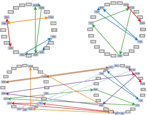
To determine the benefits of international KEPs we conduct a case study involving two countries which aim to develop a joint KEP and are concerned about the advantages and disadvantages of cooperation between their KEPs. We compare the individual benefits from the no cooperation case to the consecutive matching and merged pool scenarios. We illustrate the differences between no cooperation and merged pools cases with a small example in Fig.1.

The simulation involves 20 instances each containing the compatibility information for 1000 patient-donor pairs. For the sake of simplicity, although our model can handle altruist donors (who start chains), for the case study we only consider the cyclic exchanges among incompatible patient-donor pairs. The reason for this choice is to be able to more clearly see the difference in cooperation (because adding chains may dramatically increase the number of transplants in any given KEP stage). The length of the considered time-frame for the simulated kidney exchange scenarios is 3 years with matching runs scheduled every 3 months for each instance. Every agent is assigned an uniformly distributed arrival time to the KEP and the patient-donor pairs stay in the KEP for a maximum of 1 year (or 4 matching runs) after which they leave the programme (which means that they opt for an alternative solution, such as having a direct ABO-incompatible transplant after desensitisation or getting a deceased organ).

To understand the importance of the parameters of collaboration presented in Sect.4 we conduct a sensitivity analysis by considering most of the combinations possible.

We illustrate the impact of both programme pool size and local policy constraints on the cooperation of KEPs by:

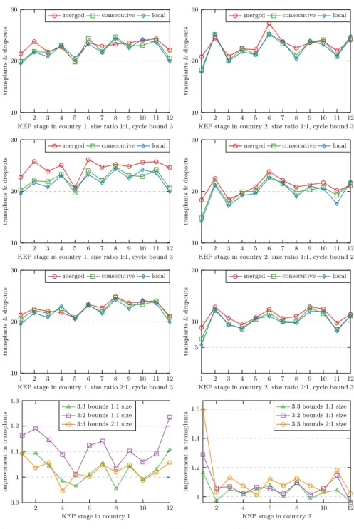
1. examining the stage-by-stage amount of transplants and drop-out patients of the programme in each country (see Fig.2).

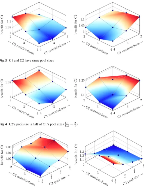
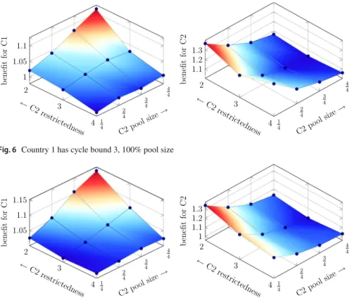
2. examining the total number of transplants resulting after 3 years for each participant country (see Figs.3,4,5,6and7).

Technical information regarding the simulations

To find the maximum number of transplants for each KEP matching problem, the state-of-the-art Gurobi solver was called from a Java implementation operating under

(12)

128 448

706

5 10301094

1163

205 781

593

1234

283 350

224 163 293

550

104 684

240

1136 884

375 509

129 1220 966

1158

586

77

462 591

272 849

727 794

96 1122

486

1194

366 300

175 947

694 759

633

953 1018

636

128 129

5

1158 1030

1163 781

272 794

283

163 293

550

1194

300 684

175 947

694

953

448 706

1220 966

1094

586

77

205

462 591

849

593

1234 727

350

96

224

1122

486 104

366 240

1136 884

759

375 633

1018

636 509

Fig. 1 Graphical illustration of two cooperating countries, each permitting at most 3-cycles. Patient-donor pairs are represented by arbitrarily labeled rectangles. Each circle configuration represents each country’s PDP pool and arcs represent planned transplants. The top side showcases the no-cooperation scenario of separate KEPs: 10/24 patients receive transplants in the left-side country, while 8/26 patients in the right- side country receive transplants. In the bottom side the pools are merged and a single optimization stage is performed for planning the transplants: the numbers are 12/24 (left) and 14/26 (right)

Ubuntu 16. More specifically, a total of 11520 KEP matching problems were solved in order to obtain the comprehensive data briefly summarized in Figs.2,3,4,5,6and 7and Tables1and2. To achieve this, a single desktop computer (i7-7700K 4.5 GHz processor and 8 GB RAM) has run for about 22 h. Thus, the average is about 7 s for solving each matching problem.

Explanation of the figures and tables

In the first row of Fig.2we consider a baseline scenario where two countries have the same pool size (on average 41.6 patients arrive per stage or 500 during 3 years) and same constraints (local and international cycle bound 3, no altruist donors).

Then, in the second row of Fig.2we demonstrate the effects of local KEP constraints on the matched pairs by only changing the local constraint in country 2 (now has local cycle bound 2 and international cooperation can be done with 2-cycles and 3- cycles with only one participant patient-donor pair in country 2). Note that the patient compatibility and arrival time to the programme was not modified.

(13)

1 2 3 4 5 6 7 8 9 10 11 12 10

20 30

KEP stage in country 1, size ratio 1:1, cycle bound 3

transplants&dropouts

merged consecutive local

1 2 3 4 5 6 7 8 9 10 11 12

10 20 30

1 2 3 4 5 6 7 8 9 10 11 12

10 20 30

1 2 3 4 5 6 7 8 9 10 11 12

10 20 30

1 2 3 4 5 6 7 8 9 10 11 12

10 20 30

1 2 3 4 5 6 7 8 9 10 11 12

5 10 20

2 4 6 8 10 12

0.9 1 1.1 1.2 1.3

KEP stage in country 1

improvementintransplants

3:3 bounds 1:1 size 3:2 bounds 1:1 size 3:3 bounds 2:1 size

2 4 6 8 10 12

1 1.2 1.4 1.6

KEP stage in country 2

improvementintransplants

3:3 bounds 1:1 size 3:2 bounds 1:1 size 3:3 bounds 2:1 size

Fig. 2 Plots detailing the amount of transplants during each stage of the KEP and separately for each country (country 1 on the left side and country 2 on the right). The first three rows each containin two plots showcasing a different scenario: (1:1 size, 3:3 bounds), (1:1 size, 3:2 bounds) and (2:1 size, 3:3 bounds), respectively. The bottom row describes individual relative improvement merged transplants

local transplants for country 1 (left) and country 2 (right)

(14)

2 3 4 2

3 4 1

1.05 1.1

C1restrictedness

←C2 →

restrictedness

2 3 4 2

3 4 1

1.05 1.1

C1restrictedness

←C2 →

restrictedness

Fig. 3 C1 and C2 have same pool sizes

2 3 4 2

3 4 1

1.05

C1restrictedness

← → C2res

trictedness

2 3 4 2

3 4 1.1

1.25

C1restrictedness

← →

C2restricte dness Fig. 4 C2’s pool size is half of C1’s pool size (^C1_C2 =²₁)

2 3

4 ¹₄

2 4

3 4

4 4

1.02 1.04 1.06

←C2

restrictedness

C2pool size→ 2

3

4 ¹₄

2 4

3 4

4 4

1.11.2 1.3

←C2

restrictedness

C2poolsize→ Fig. 5 Country 1 has cycle bound 2, 100% pool size

In the third row of Fig. 2, we show the impact of pool size on the number of transplants by only removing half of the patients inside the pool of country 2 (they never register to the KEP). Note that the patient compatibility and arrival time to the programme for the remaining patients was not modified.

Finally, the bottom row of Fig.2shows the relative improvement in the number of transplants defined as: the number of transplants obtainable by merged KEP divided by the number of transplants that would have been achieved by the respective country’s local KEP.

(15)

2 3

4 ¹₄

2 4

3 4

4 4

1 1.05 1.1

←C2

restrictedness

C2poolsize→ 2

3

4 ¹₄

2 4

3 4

4 4

1.11.2 1.3

←C2 restri

ctednes

s C2poolsize→

Fig. 6 Country 1 has cycle bound 3, 100% pool size

2 3

4 ¹₄

2 4

3 4

4 4

1.05 1.1 1.15

←C2

restrictedness

C2poolsize→ 2

3

4 ¹₄

2 4

3 4

4 4

1 1.11.2 1.3

←C2

restrictedness

C2poolsize→ Fig. 7 Country 1 has cycle bound 4, 100% pool size

In every scenario the objective is simply to maximise the number of transplants.

There are three settings for collaboration: no cooperation (i.e. separate KEPs, baseline scenario), consecutive matchings (each country runs a local KEP optimisation and then the remaining patient pools enter a joint KEP) and full collaboration (a single KEP for both countries).

Figs.3,4,5,6and7describe the improvement resulting from merged KEP collaboration. We define as benefitof collaboration for each participating country the following ratio: the number of transplanted patients belonging to a specific country obtained from merged collaboration over the number of transplants that can be achieved without any collaboration (local KEP). In this context, abenefitof 1 means no change, while 1.5 means that the number of transplants has increased by 50%.

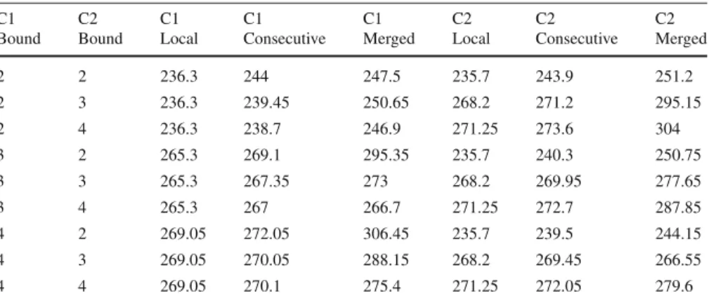
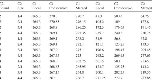
These figures are a result of a sensitivity analysis experiment where the effects of local country bounds and size limitations are explored. The information is also dis- played in numeric format in Tables1and2. The listed values represent the number of performed transplants (for each country) measured at the end of the 3 year programme and the values are averages of 20 instances (each instance runs for 12 KEP stages).

Experimental results discussion

Our experiments reveal the following observations:

(16)

Table 1 Number of transplants in each country (average of 20 instances)

C1 C2 C1 C1 C1 C2 C2 C2

Bound Bound Local Consecutive Merged Local Consecutive Merged

2 2 236.3 244 247.5 235.7 243.9 251.2

2 3 236.3 239.45 250.65 268.2 271.2 295.15

2 4 236.3 238.7 246.9 271.25 273.6 304

3 2 265.3 269.1 295.35 235.7 240.3 250.75

3 3 265.3 267.35 273 268.2 269.95 277.65

3 4 265.3 267 266.7 271.25 272.7 287.85

4 2 269.05 272.05 306.45 235.7 239.5 244.15

4 3 269.05 270.05 288.15 268.2 269.45 266.55

4 4 269.05 270.1 275.4 271.25 272.05 279.6

Same sized pools, different policy constraints

1. On average, when countries collaborate, they do not lose out in terms of total number of transplants after 3 years even without enforcing individual rationality constraints.

2. The merged KEP generally shows much better improvement in the number of transplants than the consecutive KEP for less restricted countries. The consecutive KEP seems more significant (closer to the merged KEP results) for more restricted cases (see 2:2 bound case in Table1).

3. The size of the KEP pool is a significant factor and positively impacts all forms of collaboration (see Figs.5,6and7and row 3 in Fig.2).

4. When a smaller country (in terms of KEP pool size) collaborates with a larger country, the smaller country sees greater benefit than the larger country, while the larger country usually does not lose transplants over what they can achieve by themselves.

5. All things being equal, the partner with the larger KEP pool is preferred. However, the restriction level of the partner is usually more significant to the benefit gained from collaboration. For an example on how a smaller partner is preferred if they are more restricted than an equally sized partner, refer to Fig.6: the height (benefit) at(bound,si ze)coordinates(2,³₄)is greater than the benefit at(3,⁴₄)for country 1 (left side).

6. Because of our policy to allow international cycles that are at most the length of the larger cycle bound of the two partners, we arrive at an interesting observation. It appears that it is better for a country to have a more restricted partner when they are both the same size. That is because the more restricted partner will underutilise his own KEP pool, allowing for international transplants that help the less restricted country to achieve a better outcome in terms of the number of their own transplants.

6 Conclusion

We studied the multi-country kidney exchange problem, where the participating countries may have different constraints and objectives on their national cycles and chains

(17)

Table 2 Number of transplants in each country (average of 20 instances). Country 1 has fixed pool size of 100% and cycle bound 3, Country 2 has varying pool size and varying policy constraints

C2 C2 C1 C1 C1 C2 C2 C2

Bound Size Local Consecutive Merged Local Consecutive Merged

2 1/4 265.3 270.3 270.7 47.3 50.45 64.75

2 2/4 265.3 270.85 276.15 105.2 109 127.8

2 3/4 265.3 268.8 286.25 172.3 176.65 191.45

2 4/4 265.3 269.1 295.35 235.7 240.3 250.75

3 1/4 265.3 269.1 268.2 54.9 56.8 67.8

3 2/4 265.3 269.1 272.1 121.1 123.25 133.3

3 3/4 265.3 267.9 275.1 196.6 198.45 205.45

3 4/4 265.3 267.35 273 268.2 269.95 277.65

4 1/4 265.3 268.3 262.75 56.15 58.1 75.65

4 2/4 265.3 268.65 265.95 123.7 125.75 143.2

4 3/4 265.3 267.15 264.8 200.1 202.25 219.55

4 4/4 265.3 267 266.7 271.25 272.7 287.85

and the parts of the international cycles and chains they are involved in. We formu- lated IP-models to describe various reasonable conditions by extending the classical cycle- and edge-formulation models with new segment variables and with constraints linking the three types of variables. These formulations are particularly useful if some participant country has no bounds of the lengths of the cycles or altruistic chains.

In the simulation part we tested the two-country scenario focusing on the depen- dence of the countries’ benefits on the sizes of their pools, and their restrictions. The simulations are realistic with regard to the current practices in Europe and can provide interesting consideration for the decision makers. Let us take Spain as an example, where three-way exchanges are allowed and consider its cooperation with another European country supposing that they have the same pool size. If France is the other country with cycle-length bound 2 then France will gain around 6%. For the UK with cycle-bound 3 the gain is around 3.5%, and for the Netherlands with cycle-bond the gain is around 6%.

We briefly described the way that altruistic chains can be treated in this frame- work, but in a more extensive study one could consider the particular challenges and constraints related to them. In a potential follow up paper one could also extend this study by considering also the quality of the transplants, rather than only the number of transplants, which is the primary, but not the only goal of the current kidney exchange programmes.

Acknowledgements This article is based upon work from COST Action ENCKEP: European Network for Collaboration on Kidney Exchange Programmes (CA15210), supported by COST (European Cooperation in Science and Technology); seewww.cost.eu.

Funding Open access funding provided by ELKH Centre for Economic and Regional Studies.

Open Access This article is licensed under a Creative Commons Attribution 4.0 International License, which permits use, sharing, adaptation, distribution and reproduction in any medium or format, as long as you give appropriate credit to the original author(s) and the source, provide a link to the Creative Commons licence,