Business, Housing, and Credit Cycles – The Case of Hungary*

Business, Housing, and Credit Cycles – The Case of Hungary*

Eyno Rots

This paper studies the characteristics of financial cycles in Hungary. It applies existing methodology from the literature to Hungarian data to estimate a multivariate structural time-series model. The model allows for a joint examination of the behaviour of the Hungarian financial sector and the overall economy, and estimates their cyclical positions. According to the results of the estimation, the financial sector in Hungary seems to experience volatile cycles, which last more than 15 years on average. Moreover, the cyclical position of output seems to show strong co- movement with the long financial-sector cycles. Although the data series available for Hungary are relatively short, the results of the estimation are quite credible, since they conform to the existing international evidence and seem robust to even stricter data limitations.

Journal of Economic Literature (JEL) codes: C32, E32, E44

Keywords: time-series models, financial cycles, real business cycles, house prices, MLE

1. Introduction

In the wake of the global financial crisis, economists have been paying considerable attention to macro-financial linkages. There is now a large body of empirical literature that provides conclusive evidence on the link between the financial and the real side of the economy. For example, Reinhart and Rogoff (2009) studied recessions around the world using over 800 years of data and find that they are particularly severe when they are accompanied by banking crises or rapid contractions of lending activity. Schularick and Taylor (2012) also conducted a study of crises based on long historical data and find that credit growth is a powerful predictor of a financial crisis; moreover, the ensuing recession tends to be more severe when the credit growth is rapid. Given this evidence, tracking developments in the financial sector and protecting its stability have become an important part of

many policymakers’ mandate. For the sake of an effective macroprudential policy, it has become necessary to evaluate the current state of the financial sector and its future prospects in an accurate and timely manner.

It has become evident that an economy’s financial sector activity, which can be measured by such variables as the aggregate credit volume, is subject to cyclical fluctuations. The financial sector tends to experience periods of expansion, accompanied by rising leverage, increasingly risky profit-seeking behaviour, looser lending standards, etc. Periods of expansion are followed by contractions, which may occur as financial crises, when financial institutions rapidly de-leverage and cause a collapse of the credit supply. Recent research (see Drehmann et al. 2012, Aikman et al. 2015, Galati et al. 2016, Rünstler et al. 2018) has revealed that, in many countries in Europe and elsewhere, financial cycles are longer and larger than the typical business cycles, which are believed to manifest themselves through such variables as GDP and its components, inflation and unemployment. One popular way to examine the cyclical financial sector activity is to pool data from several sources and conduct multivariate estimations. For example, house prices can serve as a good source of information on financial cycles, along with measures of credit.

There are various feedback loops between residential prices and credit aggregates, which mainly operate through the market for mortgages. For example, higher housing demand increases house prices and makes it necessary for households to take out larger mortgages in order to be able to afford housing. Higher house prices also result in a higher value of collateral available to back mortgages. Vice versa, a stronger supply of credit may boost mortgage lending and increase demand for housing. A recent example of an empirical study that jointly considers credit, house prices and GDP to extract cyclical components of these series is Rünstler and Vlekke (2018). They estimate a multivariate structural time-series model (STSM) using the data from the US and several European countries and find evidence of long and volatile financial cycles there.

The goal of this paper is to confirm the presence of long and volatile financial cycles in Hungary. It follows Rünstler and Vlekke (2018) and performs an analogous estimation for Hungarian data on GDP, total banking credit extended to private firms and households, and the house price index developed by the Magyar Nemzeti Bank (MNB). The findings conform to the evidence from other countries. Namely, the financial series (credit and house prices) exhibit long cycles, which average 14–16 years in length. Moreover, the estimation of the multivariate model reveals that the GDP series also shows pronounced medium-term fluctuations, which average about 15 years and are longer than what can be called “real business cycles”. The GDP cycles tend to comove with the financial cycles – the coherence between the two types of series is especially evident over medium-term frequencies, which are lower than business-cycle frequencies. The connection existing between the cyclical

positions of output and the financial series provides an argument for coordination between monetary and macroprudential policies. Finally, the estimation results show that the multivariate approach can provide real-time estimates that are much more accurate than univariate filters (such as the Christiano-Fitzgerald filter, for example), which means that policymakers should rely on several sources of information in order to make an accurate and timely evaluation of the cyclical position of the financial sector.

This work is by no means the first to look at cyclical developments in the Hungarian financial sector. In recent years, there has been keen interest in the assessment of financial cycles in Hungary, following the repercussions of the global financial crisis and the establishment of a comprehensive macroprudential policy framework by the Magyar Nemzeti Bank (the central bank of Hungary). Several empirical studies have provided estimates of the cyclical positions of the series related to the financial sector. Compared to the existing empirical research, the key contribution of the present work is that, to the best of my knowledge, it takes a first look at the empirical regularities of the cycles that are exhibited by the Hungarian financial sector data.

Hosszú et al. (2015) compare the ability of different filtering methods to evaluate the cyclical position of the Hungarian credit-to-GDP ratio. Between the multivariate Hodrick-Prescott (HP) filter and a set of standard univariate filters, such as Christiano-Fitzgerald, Beveridge-Nelson, and univariate HP filter, they favour the multivariate model, which tends to provide more accurate real-time estimates.

Motivated by this finding, Kocsis and Sallay (2018) use a modification of the multivariate HP filter to decompose the credit-to-GDP ratio into the unobserved cyclical and trend components. However, the authors do not estimate the cycle length. To extract a trend, they assume a value of the smoothing parameter of the HP filter, which is based on the empirical observation from the literature that financial cycles tend to be about four times as long as business cycles. On the contrary, the current work does not make such assumptions, as its goal is precisely to establish the empirical facts about the Hungarian financial cycles, including their length. Still, it conforms to Hosszú et al. (2015) and Kocsis and Sallay (2018) in the sense that it relies on a multivariate model to evaluate the financial cycles, although the model is different.

Banai et al. (2017) constructed a Hungarian house price index using the hedonic- regression approach. It covers the widest available data on housing market transactions, and it allows the national house-price level to be tracked back to 1990. Using this index, Berki and Szendrei (2017) estimate a vector error-correction model, which establishes a co-integrating relationship between the house price

by housing market fundamentals, and establish a stationary, cyclical movement of the actual house price around the equilibrium. Strictly speaking, this method is not a pure trend-cycle decomposition, because the equilibrium house price is determined by fundamentals, which experience cyclical movement of their own.

Moreover, the authors do not focus on the general properties of housing market cycles, or the financial sector more generally. Nevertheless, they do point out that the housing market gap is persistent, and that the volatility of the gap might be underestimated.

Before I describe the estimation and results, one important remark is in order. To study financial cycles, it is desirable to obtain long time series. Hungarian data, however, are only available from the early 1990s. Therefore, it is with extreme caution that we can make any judgement on the features of Hungarian financial cycles. Less than three decades of data are available, whereas international evidence suggests that these cycles may last up to 15–20 years. With this limitation in mind, I invite the reader to treat this work as an early look at the Hungarian financial cycles.

2. Methodology

The goal of the study is to use the method of Rünstler and Vlekke (2018)¹ and apply it to the Hungarian data. This method allows for the study of the cyclical behaviour of Hungary’s economy and the financial sector together, as opposed to empirical approaches that look at real business cycles and financial cycles separately. To study several data sources jointly seems appropriate, especially because the Hungarian data series are rather short. In addition, in order to cope with the problem of limited data, the results of the estimation of Hungarian cycles are cross-checked against the results reported by Rünstler and Vlekke for the US and several European economies.

For the purposes of the estimation, the dynamics of GDP, credit volume and house prices can be jointly decomposed according to the following multivariate structural time-series model (STSM):

x_t=µ_t+x_t^c+ε_t, (1) where xt is a vector that contains the values of the three variables observed in a quarter t,x_t^cis its cyclical component, μt is a trend component, and ε_t∼N

(

)

is a vector of independent and identically distributed errors. I refer the reader to the original paper (Rünstler and Vlekke 2018) for the details of the specification.

Importantly, the cyclical component is a linear combination of n cycles:

x_t^c=A!ψ!t, (2)

1 It is an extended version of the multivariate structural time-series model (STSM) due to Harvey and Koopman (1997)

where à is a matrix, and ψ!t is a stack of n cycles. Each cycle ψ!_it,i∈

{

}

1−φ_i

( )

(

)

−sinλi cosλi

⎡

⎣⎢ ⎤

⎦⎥ψ!_it−1+κ!_it. (3) In this formulation, ψ!it is a 2 x 1 vector that summarises a cycle;λ_i is a parameter that determines the frequency of the cycle; ρi is the cycle-dampening auto- regressive coefficient (high value of ρi corresponds to well-pronounced cycles of frequency λ_i); φ_i is an auto-regressive coefficient that is introduced in addition to ρ_i in order to make the model capable of capturing the persistence of financial cycles observed in the data.

The presented model specifies the cyclical behaviour of each of the observed variables as a combination of n cosine waves of various frequencies and with different phase shifts. The model’s structure makes it possible to convert the estimates of the model’s parameters into the measures of each variable’s cyclical volatility and persistence, as well as phase shifts and coherences between the three variables over various frequency ranges. I report these estimates in the results section. Note that the specification of the model described by equations (1)–(3) allows for an arbitrary number of cycles n. I use the model with three cycles: n = 3.

However, the maximum-likelihood estimation over the Hungarian data has revealed preference for the specification in which two out of three cycles of the cyclical component x_t^c are restricted to have the same parameterisation

{

}

there are cycles of two kinds that characterise the cyclical behaviour of the observed variables. Likelihood-ratio tests failed to show that allowing for three different cycles significantly improves the empirical fit of the model, whereas a more restricted model with one cycle parametrisation performs significantly worse. Therefore, I report the results obtained from a multivariate model with two different types of cycles. Intuitively, the fluctuation of each of the observed series around a trend is specified as a combination of unobserved processes that are cyclical in nature, and that have different frequencies of the cycles.

As for the trend component µt, its growth rate is driven by a combination of permanent (slope) and transitory (level) shocks:

µt=µ_t−1+β_t−1+ηt, ηt∼N

( )

( )

The 3 x 1 vector µt defines trends for the three observed variables, and independent normally-distributed shocksηt and ζt are characterised by the 3 x 3 variance-covariance matrices Σ_η andΣ_ζ. For comparability of the results with the literature, I restrict the slope innovation for each of the three variables as an independent shock (which corresponds to a diagonal variance-covariance matrix Σζ). Moreover, for credit and house price, I fix the standard deviation of the slope innovation at σ_ζ =0.005 ,² which accounts for the fact that the financial sector in Hungary, as measured through credit volumes and house prices, arguably has experienced volatile trend dynamics since the transition to a market-based economy.³

In order to estimate the model, I cast the model in its state-space form and therefore make it possible to implement the Kalman filter and compute the likelihood function for a certain parameterisation of the model given the observed data. I rely on Newton-based numerical methods to maximise the likelihood function and find the maximum-likelihood estimates of the model’s parameters and the corresponding measures of the cyclical behaviour of the observed variables.

The performance of the multivariate model is also compared against the set of three univariate models (one individual cycle independently estimated for each of the variables). Technically, the difference between the two cases is whether the non-diagonal elements of matrix A! in equation (2) are restricted to be zero (in case of univariate models) or not. Unlike the set of univariate models, a multivariate model allows the possibility of interactions between the cyclical components of the variables under consideration. In terms of the achieved values of the likelihood function, the multivariate model, in which cycles jointly determine the cyclical behaviour of all three variables, performs significantly better than a stack of three univariate models. I therefore focus on reporting the results for the multivariate model below.

3. Results

I obtain quarterly Hungarian data that spans 1990q1–2018q1 and includes real GDP, aggregate credit volume extended by domestic banks to the private sector, and the MNB house price index.⁴ As already noted, the data series available for Hungary are less than 30 years long; it is quite an audacious task to rely on such short data series to judge about the empirical features of financial cycles that are likely to last longer than 15 years. Nevertheless, the results obtained for Hungary are in line with the findings for other European countries reported in the existing

2 Rünstler and Vlekke (2018) set the values between 0.001 and 0.0025.

3 For example, see Berki and Szendrei (2017).

4 All data are adjusted for inflation and seasonally, where necessary. Sources: BIS, Eurostat, MNB, KSH.

literature and qualitatively robust to even stricter data limitations, which definitely adds some credibility to the findings reported below.

The estimation of the multivariate model with two cycles suggests that the cyclical behaviour of the observed series is driven by cycles with average lengths of 2.8 and 19.4 years. However, the average length of each individual cycle ψ!_it is difficult to interpret: according to equation (2), the cyclical component of each of the observed variables is a linear combination of the two cycles. For this reason, instead of the individual cycles and their parameter values, I report the results in terms of the combined cyclical behaviour of the observed variables, such as average cycle length, volatility, etc.

Table 1

Cyclical properties of the observed variables in Hungary

Variable

Y_t C_t P_t

Cycle length, years 16.940 15.091 15.693

Cycle volatility, per cent 8.612 20.052 18.261

Note: Cyclical properties of the observed variables: GDP (Y_t), credit (C_t) and house price (P_t). The table shows estimates of the average length and the standard deviation of the cycles observed in each of the three variables. These values are obtained using the multivariate spectral generating function from the estimates of the parameters that characterise the cyclical component of the model.

Table 1 reports the average cyclical behaviour of the GDP (Yt), the volume of credit (C_t) and the house price (P_t) estimated for Hungary. The house-price and credit cycles are estimated to last 15–16 years and be 2–2.5 times as volatile as the output cycles. The standard deviation is estimated to be 18.3 per cent for the house price cycles and 20.1 per cent for the credit cycles, whereas for the GDP cycles it is 8.6 per cent. As already mentioned, the estimated length of the cycles is large compared to the length of the available data, which may raise doubts about the quantitative precision of the findings. However, as discussed in section 4.2 below, an estimation over a much shorter data set delivers results that are qualitatively very similar for Hungary, which is reassuring for the validity of the findings.

It is also somewhat reassuring that the presented findings are in line with the existing empirical evidence. For Hungary, a good reference would be the evidence from CEE countries, which, unfortunately, is limited. For example, Gonzalez et al.

(2015) try to estimate the length of credit and business cycles in 28 countries, but for the CEE countries in their sample (Czech Republic, Hungary, Poland), they are unable to find evidence of long cycles, which is due to the fact that the available data series are short for these countries. Communale (2017) does report that house price and credit cycles are more volatile than the GDP cycles in Estonia, Croatia, Hungary, Latvia, Lithuania, and Slovenia, but does not report the cycle durations.

Nevertheless, evidence from other countries suggests the presence of financial cycles that are generally longer than the business cycles, which are typically assumed to last 2–8 years, and much more volatile. Rünstler and Vlekke (2018) estimate the cyclical behaviour of GDP, credit, and house price for several European countries and the US: in all countries but Germany, they find that the financial series exhibit cycles that are much longer than the output cycles, and last between 11.8 and 18.7 years on average. As for Germany, its financial series feature short cycles, which fall within the business-cycle range, and which are about as volatile as the cyclical fluctuations of GDP. Interestingly, the authors also report that countries with higher homeownership rates tend to have longer and more volatile financial cycles. A potential reason for this relationship may be that high homeownership

Figure 1

Homeownership and financial cycles

US UK

DE FR

IT ES

HU

50% 60% 70% 80% 90% 100%

Cycle length, years

Homeownership rate Credit House price

US UK

DE

FR IT

ES HU

50% 60% 70% 80% 90% 100%

Cycle volatility, per cent

Homeownership rate Credit House price 0

2 4 6 8 10 12 14 16 18 20

0 5 10 15 20 25 30

Note: Relationship between the homeownership rate and the cyclical behaviour of the house price and the credit volume. Estimates for Hungary (black marks) are added to the existing estimates of Rünstler and Vlekke (2018) for other European countries and the US.

rate is a symptom of low liquidity of the housing market,⁵ which results in sluggishness of house price dynamics and, through the relationship between the markets for housing and mortgages, of the credit-volume dynamics. Regardless of the explanation, Germany seems to follow this pattern, since it is a country with a very low homeownership rate, which was at only 52 per cent on average between 1995 and 2013. In Figure 1, I augment the data from Rünstler and Vlekke with the Hungarian numbers: it appears that these numbers fit the general picture. The Hungarian house price and credit cycles seem to be comparatively long and volatile, but the Hungarian homeownership rate is also the highest among the reported economies: according to the population surveys conducted by the country’s Central Statistical Office (Központi Statisztikai Hivatal, KSH) in the last decade, over 90 per cent of the households own the dwellings where they live.

Speaking about the GDP cycles, Table 1 shows them to be quite long in general. In line with the aforementioned empirical literature, the Hungarian GDP cycles also tend to be longer than what is typically believed to be the business-cycle range of 2–8 years. They are estimated to last 16.9 years on average. This empirical finding is difficult to establish by means of the commonly used univariate Hodrick-Prescott, Baxter-King, and Christiano-Fitzgerald filters. These filters require an assumption about the plausible range of cyclical frequencies in order to extract the cyclical component. Naturally, if the initial assumption is that the cyclical component only includes cycles that last 2–8 years, it is impossible to extract cycles with lower frequencies from the data. So, the first limitation of the aforementioned filters is that they depend on such an assumption. The second limitation is that they only consider the series individually. Given that the available data series are often rather short, it may be difficult to identify low-frequency cycles from such data series, even if the researcher has no prior assumptions about the plausible cycle length. When the cycle length is sizable compared to the length of the available data series, it may be necessary to pool several data series together in order to discover such a cycle.

By looking at the dynamics of GDP together with house price and credit volume, it is possible to uncover medium-term fluctuations. These fluctuations occur at frequencies that are lower than the frequencies of the real business cycles, the traditionally assumed domain of GDP. In addition, by looking at the data jointly, it is possible to establish a high degree of comovement between the medium-term GDP and financial cycles.

Table 2

Coherence between cyclical components in Hungary

Y_t, C_t Y_t, P_t C_t, P_t

Total 0.851 0.245 0.371

8–32 quarters 0.461 0.128 0.352

32–120 quarters 0.891 0.257 0.379

Note: Coherence between the cyclical components of the observed variables: GDP (Y_t), credit (C_t) and house price (P_t).

Table 2 shows pairwise coherences between the three observed variables, which is the counterpart of correlation that is computed over the frequency domain using spectral analysis: it allows us to check over which frequencies (or which cycle lengths) the variables exhibit the greatest comovement. The close connection between the financial cycles and GDP is evident for the credit volume: while the coherence between GDP and house price is 0.245, it is as high as 0.851 between GDP and credit. Moreover, the financial variables seem to have stronger coherence with GDP in the medium term rather than the short term. Coherence over cycles lasting 8–32 quarters is estimated to be 0.461 between GDP and credit and 0.128 between GDP and house price, while the corresponding figures for medium-term frequencies, or cycles lasting 32–120 quarters, are 0.891 and 0.257.

Figure 2 demonstrates estimated cyclical components of GDP, credit volume and house price. The cyclical components panel shows the cycles for the three variables together. It is evident that within the multivariate STSM that is estimated for Hungary, there is visible comovement between the GDP cycles and the financial cycles (summarised by the other two variables). The cyclical position of GDP shows persistence, and it generally maintains the same sign and similar changes as the cycles of the financial variables. The last two panels of Figure 2 compare the cyclical positions of GDP and house prices estimated using the multivariate STSM with the official, publicly-available estimates. The GDP panel compares the GDP cycle with the quarterly estimates of the output gap provided by the MNB (data available from 2002) and with the annual data for the output gap provided by the OECD (available from 1996).⁶ According to the estimated model, the output gap was persistently positive in Hungary before 2008, when the global financial crisis unfolded and the gap turned negative. This timeline is very similar to the official figures. Unlike the official data, however, the estimates from the STSM indicate that the output gap still remained negative at the end of 2017, although it had been consistently shrinking since 2012. Overall, the model’s estimates of the output gap are qualitatively similar to the official estimates.

6 OECD annual data are interpolated in order to obtain quarterly figures.

Figure 2

Cyclical positions of GDP, house price and credit in Hungary

1.4 1.6 1.8 2.0 2.2

1990 1992 1994 1996 1998 2000 2002 2004 2006 2008 2010 2012 2014 2016 2018 GDP, logged

Trend Series

5.5 5.0 4.5 4.0 3.5 3.0

1990 1992 1994 1996 1998 2000 2002 2004 2006 2008 2010 2012 2014 2016 2018 Credit volume, logged

Trend Series

4.0 4.5 5.0 5.5

1990 1992 1994 1996 1998 2000 2002 2004 2006 2008 2010 2012 2014 2016 2018 House price, logged

Trend Series

60 40 20 0 –20 –40 –60

1990 1992 1994 1996 1998 2000 2002 2004 2006 2008 2010 2012 2014 2016 2018

1990 1992 1994 1996 1998 2000 2002 2004 2006 2008 2010 2012 2014 2016 2018 Cyclical components, %

House price

GDP Credit

20 10 0 –10 –20

1990 1992 1994 1996 1998 2000 2002 2004 2006 2008 2010 2012 2014 2016 2018 Estimates of GDP cycle, %

MNBModel

40 20 0 –20 –40 –60

Estimates of the house price cycle, %

MNBModel OECD

There are more visible deviations concerning the size and the sign of the estimated house price cycle when it is compared with MNB’s estimate of the deviation of the house price index from the level “justified by the macroeconomic fundamentals”⁷. The reason for that seems to be the fact that the trend estimated by the STSM does not account for fundamentals. For example, the STSM is able to capture a long period of house price decline in the 1990s as a trend development, which seems to be the case:

Hungary was undergoing a transition from a planned economy. The cyclical deviation is relatively moderate for that period. On the contrary, there was a period of house price growth around the early 2000s, which was in part due to rising income per capita, and in part due to the development of the mortgage market and introduction of mortgages subsidised by the government during that period. These developments can be captured as fundamental in the MNB’s official estimates, resulting in a rising equilibrium house price and a smaller positive house price gap. At the same time, the STSM is likelier to treat the house price movement in the early 2000s as cyclical, which results in a larger cyclical deviation compared to the official estimates. Similarly, upon the outbreak of the 2008 crisis, there was a fall in household incomes, the emergence of non-performing mortgage loans, especially FX-denominated loans in the face of a weakening forint, and the ensuing tightening of lending conditions.

These fundamental developments could be treated as a decrease in the equilibrium house price, which effectively postponed the time when the official price gap became negative, whereas the STSM model is likely to interpret these developments as cyclical and therefore predict an earlier change in the sign of the house price cycle. In light of these differences, it is arguable whether some of the events in the financial market, such as the development of a competitive mortgage market in the 2000s, should be viewed as permanent trend adjustments. At least part of such changes can be due to cyclical considerations – for example, it does not seem to be a coincidence that the development of the mortgage market had to take place during relatively tranquil times of credit-market expansion rather than during the financial crisis.⁸

Speaking about the discovered persistence of cycles, it is easy to miss this when employing popular univariate filters to extract cyclical dynamics. As an example, let us consider the estimates of the output gap. Figure 3 compares the estimates of the GDP cycle from the multivariate STSM with the estimates obtained using popular univariate filters. The Christiano-Fitzgerald (CF) filter is a univariate band-pass filter, which requires that the researcher specify a frequency band, or a range of frequencies of cycles to be extracted from the time series. If I assume that the cyclical output fluctuations are between 8 and 32 quarters, as is typically done in the RBC literature, I am not able to find persistent GDP cycles. Similarly, the univariate Hodrick-Prescott filter with standard parameterisation for quarterly data (λ = 1,600) is designed so that it ignores low-frequency dynamics and produces an estimate of the GDP cycle that also

7 Housing Market Report, November 2017, MNB.

8 For a more detailed discussion of the developments in the Hungarian housing markets, see Berki and

lacks persistence. By contrast, if I assume that GDP involves medium-term cycles that last between 32 and 120 quarters and run the CF filter with such band specification, I get an estimate that is much more similar to the estimate of the multivariate model.

4. Robustness checks

4.1. Precision of the real-time estimates

In the previous figures, all of the estimates of the cyclical positions of the observed variables are based on all of the available data. Looking ten years back, we can quite confidently say that, for example, the GDP gap was positive before the global financial crisis and turned negative during the crisis. However, it would be interesting to see if the same could be said just as confidently back in 2008, when the data was available only up to 2008. A policymaker does not have the benefit of hindsight and must judge about the state of the world based on current data.

To gauge the precision of the estimates of the cyclical positions of the three observed variables produced by the STSM, I follow Rünstler and Vlekke (2018) and perform the pseudo-real-time estimation of the current cyclical position of the data. To put it in terms of the model presented above, the cyclical components plotted in Figures 2 and 3 are smoothed estimates based on all of the available data, which we can denote as ˆx_{t T}^c , where T is the last quarter when the data are

Figure 3

Various estimates of the GDP gap in Hungary

–20 –15 –10 –5 0 5 10 15

–20 –15 –10 –5 0 5 10

Per cent Per cent 15

1990 1992 1994 1996 1998 2000 2002 2004 2006 2008 2010 2012 2014 2016 2018

STSM model HP filter CF filter, 8–32 CF filter, 32–120

Note: Estimates of the cyclical position of GDP obtained from the STSM model and compared with esti- mates based on standard univariate filters: Christiano-Fitzgerald filter (CF) with frequency band set between 8 and 32 quarters; CF filter with frequency band 32–120 quarters; Hodrick-Prescott (HP) filter with standard value of the smoothing parameter recommended for quarterly data: λ = 1,600.

it with another estimate ˆx_{t t+20}^c , which incorporates an additional 20 quarters of data after period t – this benchmark can be thought of as a revision of the initial real-time estimate after 5 years.

Figure 4 plots the pseudo-real-time estimates of the GDP, credit and house price cycles, together with their revisions after 5 years. Naturally, the revision is not available for the last 5 years, because this revision requires 5 years of data available after the “real-time” estimate is made. Note that both estimates use the model parameters that are estimated for the entire available data set, so the discrepancy between the two does not account for parameter uncertainty. We can see that the

“real-time” estimates are visibly close to their revised values for all three variables.

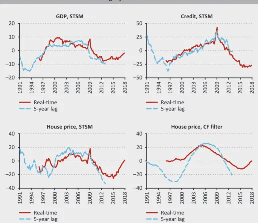
Figure 4

Pseudo-real-time estimates for Hungary

–20 –10 0 10

20 GDP, STSM

Real-time 5-year lag

–50 –25 0 25

50 Credit, STSM

Real-time 5-year lag

–40 –20 0

20 40

1991 1994 1997 2000 2003 2006 2009 2012 2015 2018 1991 1994 1997 2000 2003 2006 2009 2012 2015 2018

1991 1994 1997 2000 2003 2006 2009 2012 2015 2018

1991 1994 1997 2000 2003 2006 2009 2012 2015 2018

House price, STSM

Real-time 5-year lag

–40 –20 0 20

40 House price, CF filter

Real-time 5-year lag

Note: Pseudo-real-time estimates of the cyclical components of the three observed variables, compared with their revisions after 5 years, based on the estimated structural time-series model (STSM). The last panel shows the univariate estimates based on the Christiano-Fitzgerald filter (CF) with the frequency band set to 32–120 quarters.

Of course, there is a degree of imprecision in the real-time estimates. For example, Rünstler and Vlekke (2018) report that across the European countries and the US, the sample standard deviations of the cyclical components are about 30 per cent lower on average for the pseudo-real-time estimates than the sample standard deviations for the revised estimates. In other words, the real-time estimates tend to under-estimate the cyclical deviations. This is a well-known feature of statistical methods that decompose time series into trends and cycles: these methods tend to rely heavily on the tails of the time series to measure the trend and are therefore less likely to discover cyclical dynamics at the end of the time series than in the middle of it. The “real-time” estimates for Hungary also show a downward bias, especially for the financial series: they tend to be closer to zero than the revised estimates. However, the multivariate model performs much better than the commonly used univariate filters. To illustrate this point, I construct the pseudo-real- time estimate and the 5-year revision of the house price cycle using the univariate Christiano-Fitzgerald filter with the frequency band set to 32–120 quarters and plot the two series in the last panel of Figure 4. It is evident that the univariate filter performs worse: the real-time estimate shows a much more pronounced downward bias, and the revisions are substantial over the entire sample. As the series are too short, and due to space constraints, I refrain from reporting the statistics for the pseudo-real-time estimates. It should be noted that they are in line with Rünstler and Vlekke (2018) – and with a more general result established by the empirical literature that multivariate estimates of the cycles are more precise than univariate filters (for example, see Watson 2007). Nevertheless, even when relying on multivariate estimates, policymakers should be concerned with the downward bias of the real-time estimates of the cyclical positions of the economy and its financial sector, and thus with the possibility of missing the right moment to act.

4.2. Poor quality of the early data

When estimating the STSM model, I have relied on all the available observations for GDP, credit volume and house prices, trying to collect as long a data set as possible.

Even with this approach, the earliest available Hungarian figures for the three series jointly is the first quarter of 1990. The fact that the data series available for Hungary are rather short is a concern for the validity of the results of the estimation, as already mentioned. Moreover, an additional weakness of the data set is that the earlier observations are of quite poor quality. With regard to the house price index, its values for the 1990s are computed based only on data from Budapest. As for the credit volumes, their estimates are also questionable for the 1990s, when the credit market was transitioning towards a free market, together with the rest of the economy. As an additional check for the robustness of the results to the shortness of the data and to the poor quality of the initial observations, I repeat the maximum-

Table 3

Cyclical properties of the observed variables in Hungary, short data Variable

Y_t C_t P_t

Cycle length, years 18.753 17.635 18.094

Cycle volatility, per cent 11.077 25.234 18.535

Note: Cyclical properties of the observed variables: GDP (Y_t), credit (C_t) and house price (P_t). The table shows estimates of the average length and the standard deviation of the cyclical components of the model obtained using the data between 2000q1–2018q1.

Table 3 contains the key results of the estimation. There are sizable quantitative differences between the results of this experiment and the estimation over the full data set reported in Table 1. Qualitatively, however, the results are the same: house price and credit exhibit cycles longer than 15 years on average; the financial series are 2–2.5 times as volatile as GDP; the GDP cycles are longer than what is believed to be the business-cycle range of 2–8 years. Figure 5 plots the cyclical positions of the three observed series based on the shorter data series and compares them with the estimates based on the full data set presented in Figure 2. With the exception of the volatility of the GDP cycles, we can see that both estimates are very similar.

This result is reassuring. Despite the fact that the Hungarian data is rather short, we can see that the STSM produces robust estimates, and the characteristics of the Hungarian financial cycles can be approximately measured even using a shorter data set.

Figure 5

Estimates of cyclical components – short and long data

1990 1994 1998 2002 2006 2010 2014 2018

Full data Short data –20 –15

–10 –5 10 15 20 0 5 GDP cycles, %

1990 1994 1998 2002 2006 2010 2014 2018

Full data Short data Credit cycles, %

1990 1994 1998 2002 2006 2010 2014 2018

Full data Short data –60

–45 –20 0 20

40 House price cycles, %

–60 –40 –20 0 20 40 60

Note: Estimates of the cyclical components of the three observed variables produced using the data between 2000q1–2018q1 and compared with estimates produced using the full data set between 1990q1–2018q1.

5. Conclusion

Following Rünstler and Vlekke (2018), I conduct an estimation of a multivariate structural time-series model using the Hungarian data, in order to establish the characteristics of the Hungarian financial cycles, as summarised by the dynamics of the volume of private banking sector credit and house prices. Although the data available for Hungary are short, I manage to produce evidence of persistent financial cycles consistent with the international empirical evidence. Robustness checks indicate that even a short data set that is available for Hungary is sufficient to characterise its financial cycles. The estimation also reveals that the cyclical behaviour of GDP is related to the financial cycles, since there is strong medium- term coherence between output and the financial series. At the same time, it is easy to miss medium-term cyclical output fluctuations and their relation to the financial cycles when using the popular univariate filters. The Hungarian data suggests relatively long and volatile financial cycles – at the same time, Hungary happens to be the country with a very high home ownership rate, which puts the evidence from Hungary in line with the findings for other countries. Also in line with the existing literature, the findings suggest that the multivariate model is capable of producing real-time estimates of the cycles that are more precise than the estimates coming from univariate filters.

In terms of the policy implications, a few points are in order. The established connection between GDP and the financial cycle may serve as an additional argument for coordination between monetary and macroprudential policy. For the purposes of timely and, importantly, accurate decision-making, the findings argue for pooling the data together and relying on multivariate estimates. Finally, substantial differences between the features of the financial cycles in different countries may provide guidance for country-specific macroprudential policies.

References

Aikman, D. – Haldane, A.G. – Nelson, B.D. (2015): Curbing the credit cycle. The Economic Journal, 125(585): 1072–1109. https://doi.org/10.1111/ecoj.12113

Banai, Á. – Vágó, N. – Winkler, S. (2017): The MNB’s house price index methodology. MNB Occasional Paper 127.

Berki, T. – Szendrei, T. (2017): The cyclical position of housing prices – a VECM approach for Hungary. MNB Occasional Paper 126.

Drehmann, M. – Borio, C.E.V. – Tsatsaronis, K. (2012): Characterising the Financial Cycle:

Galati, G. – Hindrayanto, I. – Koopman, S.J. – Vlekke, M. (2016): Measuring financial cycles with a model-based filter: Empirical evidence for the United States and the euro area. DNB Working Paper No. 495. https://doi.org/10.2139/ssrn.2722547

Gonzalez, R.B. – Lima, L. – Marinho, L. (2015): Business and Financial Cycles: an estimation of cycles’ length focusing on Macroprudential Policy. Banco Central do Brasil Working Paper 385.

Harvey, A.C. – Koopman, S.J. (1997): Multivariate structural time series models. In: Heij, C. – Schumacher, J.M. – Hanzon, B. – Praagman, C. (ed.): System Dynamics in Economics and Financial Models. New York: Wiley, pp. 269–285.

Hosszú, Zs. – Körmendi, Gy. – Mérő, B. (2015): Univariate and multivariate filters to measure the credit gap. MNB Occasional Paper 118.

Kocsis, L. – Sallay, M. (2018): Credit-to-GDP gap calculation using multivariate HP filter. MNB Occasional Paper 136.

Reinhart, C.M. – Rogoff, K.S. (2009): This time is different: Eight centuries of financial folly.

Princeton University Press.

Rünstler, G. – Vlekke, M. (2018): Business, housing, and credit cycles. Journal of Applied Econometrics, 33(2): 212–226. https://doi.org/10.1002/jae.2604

Rünstler, G. – WGEM Team on Real and Financial Cycles (2018): Real and financial cycles in EU countries - Stylised facts and modelling implications. ECB Occasional Paper No. 205.

Schularick, M. – Taylor, A.M. (2012): Credit booms gone bust: Monetary policy, leverage cycles, and financial crises, 1870–2008. American Economic Review, 102(2): 1029–1061.

https://doi.org/10.1257/aer.102.2.1029

Watson, M. (2007): How accurate are real-time estimates of output trends and gaps? Federal Reserve Bank of Richmond Economic Quarterly, 93(2): 143–161.