CERS-IE WORKING PAPERS | KRTK-KTI MŰHELYTANULMÁNYOK
INSTITUTE OF ECONOMICS, CENTRE FOR ECONOMIC AND REGIONAL STUDIES, BUDAPEST, 2020
Trading Networks with Frictions
TAMÁS FLEINER – RAVI JAGADEESAN
ZSUZSANNA JANKÓ – ALEXANDER TEYTELBOYM
CERS-IE WP – 2020/8
February 2020
https://www.mtakti.hu/wp-content/uploads/2020/01/CERSIEWP202008.pdf
CERS-IE Working Papers are circulated to promote discussion and provoque comments, they have not been peer-reviewed.
Any references to discussion papers should clearly state that the paper is preliminary.
Materials published in this series may be subject to further publication.
ABSTRACT
We show how frictions and continuous transfers jointly affect equilibria in a model of matching in trading networks. Our model incorporates distortionary frictions such as transaction taxes, bargaining costs, and incomplete markets. When contracts are fully substitutable for firms, competitive equilibria exist and coincide with outcomes that satisfy a cooperative stability property called trail stabity. In the presence of frictions, competitive equilibria might be neither stable nor (constrained) Pareto-efficient. In the absence of frictions, on the other hand, competitive equilibria are stable and in the core, even if utility is imperfectly transferable.
JEL codes: C62, C78, D47, D51, D52, L14
Keywords: Trading networks; frictions; competitive equilibrium; matching with contracts; trail stabity; transaction taxes; commission
Tamás Fleiner
Department of Computer Science and Information Theory, Budapest University of Technology and Economics
and
Institute of Economics, Centre for Economic and Regional Studies, Hungarian Academy of Sciences
e-mail: fleiner@cs.bme.hu Ravi Jagadeesan
Harvard Business School; and Department of Economics, Harvard University e-mail: ravi.jagadeesan@gmail.com
Zsuzsanna Jankó
Department of Mathematics, University of Hamburg e-mail: zsuzsanna.janko@uni-hamburg.de
Alexander Teytelboym
Department of Economics, Institute for New Economic Thinking, and St.~Catherine's College, University of Oxford
alexander.teytelboym@economics.ox.ac.uk
Kereskedelmi hálózatok súrlódásokkal FLEINER TAMÁS – RAVI JAGADEESAN
JANKÓ ZSUZSANNA – ALEXANDER TEYTELBOYM
ÖSSZEFOGLALÓ
Megmutatjuk, hogy a kereskedelmi hálózat modellben mind a súrlódás, mind a folytonos átválthatóság megléte hogyan befolyásolja a közgazdasági egyensúlyt.
Modellünkben a torzítást eredményező súrlódási tényezők lehetnek tranzakciók után fizetendő illetékek, az alkufolyamathoz kapcsolódó költségek vagy hiányos piacok.
Amennyiben a modellben szereplő cégek számára az egyes szerződések korlátlanul helyettesíthetők, úgy mindig létezik közgazdasági egyensúly, és megegyezik a trail- stabilitásnak elnevezett kooperatív stabilitási tulajdonságot teljesítő végeredményekkel. Súrlódás megléte esetén azonban a közgazdasági egyensúlyi sem nem feltétlenül stabil, sem pedig nem feltétlenül Pareto-optimális. Súrlódás hiányában azonban a közgazdasági egyensúly akkor is stabil és mag-tulajdonságú, ha a hasznosság nem tökéletesen átváltható.
JEL: C62, C78, D47, D51, D52, L14
Kulcsszavak: kereskedelmi hálózatok, súrlódás, versenyző egyensúly, tranzakciós adó
Trading networks with frictions
TAMÁS FLEINER RAVI JAGADEESAN ZSUZSANNA JANKÓ ALEXANDER TEYTELBOYM
We show how frictions and continuous transfers jointly affect equilibria in a model of matching in trading networks. Our model incorporates distortionary frictions such as transaction taxes, bargaining costs, and incomplete markets. When contracts are fully substitutable for firms, competitive equilibria exist and coincide with outcomes that satisfy a cooperative stability property calledtrail stability. In the presence of frictions, competitive equilibria might be neither stable nor (constrained) Pareto-efficient. In the absence of frictions, on the other hand, competitive equilibria are stable and in the core, even if utility is imperfectly transferable.
1 INTRODUCTION
Interdependence and specialization of production are central features of the modern economy. Many firms have complex, bilateral relationships with dozens of buyers and suppliers. The terms of these relationships are typically encoded in complexcontractsthat specify goods traded or services rendered, delivery dates, penalties for non-completion, and, of course, prices. Markets that involve heterogeneous and highly specialized contracts, talented workers, or sophisticated machines can often be concentrated and thin. In such markets, it isà prioriimplausible to assume that agents act as price-takers.
Models of matching with contracts, inspired by the work of Gale and Shapley [1962], elegantly capture interaction in thin markets [Crawford and Knoer, 1981, Hatfield and Milgrom, 2005, Kelso and Crawford, 1982, Roth, 1984]. Matching models do not typically assume that agents are price-takers: instead, agents are free to engage in highly specific contracts and rely on the consent of counterparties to maintain contractual relationships. The equilibrium concepts employed in the matching literature, such asstability, require that recontracting should not be profitable. Unlike typical general equilibrium models, matching models can also incorporate indivisibilities, which are often present in thin markets. Finally, matching models capture frictions, such as transaction taxes [Dupuy et al., 2017], bargaining costs [Galichon et al., 2018], and the incompleteness of the financial market [Jagadeesan, 2017].1
While cooperative solution concepts are well-founded thin markets, competitive solution concepts are often more natural in thick markets [Edgeworth, 1881, Kelso and Crawford, 1982]. Nevertheless, competitive and cooperative solution concepts are both appealing to some extent in markets of all sizes. For example, competitive equilibrium could be a reasonable solution concept even in thin markets because it does not require firms to coordinate directly with one another. Cooperative solutions, on the other hand, offer a credible foundation for the analysis of thick markets that cannot clear—for example, due to price controls.2
This paper establishes an equivalence between competitive equilibrium and an intuitive stability concept in markets with frictions. As we will argue, our equivalence result provides new cooperative foundations for competitive equilibrium and competitive foundations for our stability concept. We also show how frictions matter for the connection between competitive and cooperative solution concepts.
We focus on trading networks to capture complex production linkages. Following Ostrovsky [2008], Hatfield and Kominers [2012], Hatfield et al. [2013], and Fleiner et al. [2018b], we assume that agents interact via an exogenously
1The financial market isincompleteif agents suffer from uninsurable risk—that is, if there is some Arrow [1953] security that is absent or cannot be traded without transaction costs.
2See Drèze [1975], Hatfield et al. [2012, 2016], Andersson and Svensson [2014], and Herings [2015].
specified set of bilateraltrades—which specify who is trading, what good or service is being traded, and any non- pecuniary parameters of exchange. Trades have directions that correspond to the flow of goods: upstream trades represent purchases and downstream trades represent sales. In a market outcome, transfers are made for every realized trade, encapsulating the role of money in the economy [Hatfield et al., 2013]. We summarize outcomes as a set of realizedcontracts, each of which specifies a trade and a price.
Our model can capture distortionary frictions in reduced form. Formally, we allow agents to place different values on transfers associated to different trades. Intuitively, when frictions are present, receiving one unit of transfer may not fully offset the cost of paying one unit of transfer. For example, transaction taxes and bargaining costs cause there to be a wedge between payment and receipt. There might also be wedges between forms of transfer when financial markets are incomplete. For example, if transfers are in trade credit that is subject to imperfectly-insurable default risk, then creditors value payments less than debtors. Similarly, if currency markets are imperfect, then firms may value local currency more than foreign currency. However, like in general equilibrium models, we assume that transfers associated to trades are one-dimensional, so that each realized trade has a well-defined price. This uni-dimensionality condition rules out partial financing of purchases with trade credit and requires that each trade is priced in a single currency [Jagadeesan, 2017].
Our first main result provides sufficient conditions for the existence of competitive equilibria. The key assumption is that preferences over contracts arefully substitutable[Hatfield and Kominers, 2012, Hatfield et al., 2013, Ostrovsky, 2008]—that is, that upstream (resp. downstream) trades are grossly substitutable for each other, and that upstream and downstream trades are grossly complementary to one another. Full substitutability can be regarded as the requirement that the goods that flow in trades are grossly substitutable [Baldwin and Klemperer, 2018, Hatfield et al., 2019]. In our model, full substitutability and a mild regularity condition together ensure that competitive equilibria exist.3
To relate the competitive and cooperative approaches to the analysis of markets with frictions, we first explore cooperative interpretations of competitive equilibria. We show that competitive equilibrium outcomes are always trail-stable—i.e., immune to sequential deviations in which a firm that receives an upstream (resp. downstream) contract offer can either accept the offer outright or make an additional downstream (resp. upstream) contract offer [Fleiner et al., 2018b]. Trail stability is a natural extension of Gale and Shapley’s (1962) pairwise stability property to trading networks.
Other solution concepts in matching theory arestability(in the sense of Hatfield et al. [2013])—which requires that there is no group of firms that can commit to recontracting among themselves (possibly while dropping some existing contracts)—and thecore. However, in the presence of frictions, competitive equilibrium outcomes are typically neither stable nor in the core.
Stable and trail-stable outcomes, on the other hand, have competitive interpretations. We say that an outcomeliftsto a competitive equilibrium if the outcome can be supported by competitive equilibrium prices—as an outcome already specifies the prices of realized trades, showing that an outcome lifts to a competitive equilibrium amounts to specifying equilibrium prices for unrealized trades. We show that trail-stable and stable outcomes lift to competitive equilibria under full substitutability and regularity conditions.4 In the presence of frictions, therefore, the trail stability and competitive equilibrium solution concepts are essentially equivalent, but they both differ from stability.
3As Hatfield and Kominers [2012] and Hatfield et al. [2013] show, full substitutability is necessary (in the maximal domain sense) for the existence of equilibria in trading networks.
4Hatfield et al. [2013] show that stable outcomes lift to competitive equilibria under full substitutability in transferable utility economies. Our results apply even in the presence of frictions and income effects.
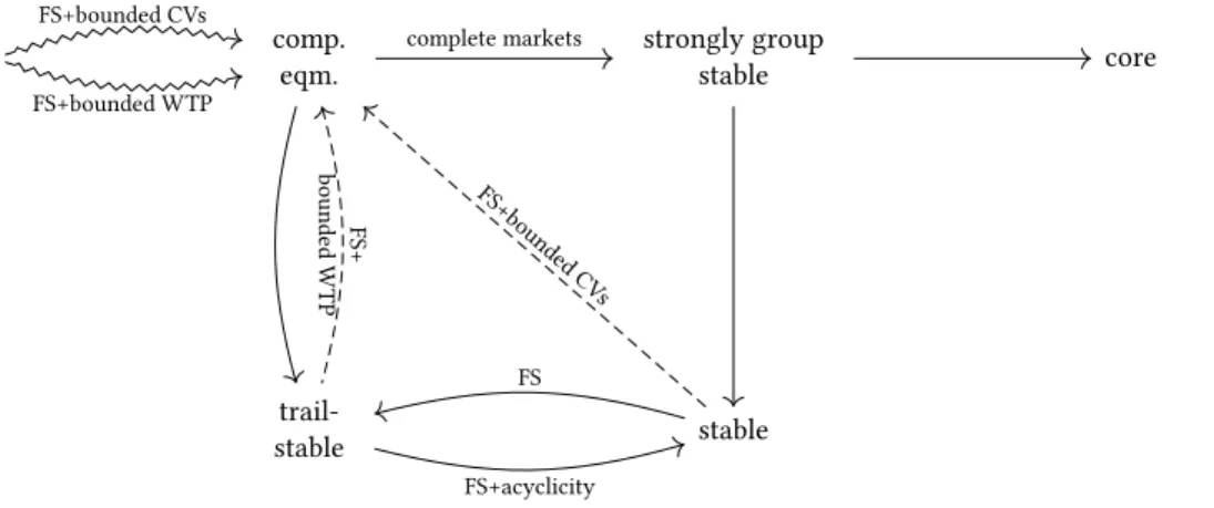
comp.
eqm.
strongly group stable
core
trail- stable
stable
FS+bounded CVs
FS+bounded WTP
complete markets
boundedWTP FS+
FS+acyclicity FS FS+b
ounde d
CV s
Fig. 1. Summary of our results. The squiggly arrows represent existence results, the ordinary arrows represent relationships between solution concepts, and the dashed arrows shows lifting results. Arrows are labeled by the hypotheses of the corresponding results. FS stands for full substitutability (see Assumption 1), “Bounded CVs" stands for “bounded compensating variations" (see Assumptions 2 and 20), and “bounded WTP" stands for “bounded willingness to pay" (see Assumption 3).
The relationship between stability and competitive equilibria changes dramatically in the absence of distortionary frictions. In this case, there are no wedges between payments and receipts, and we say that the market iscomplete.5 Completeness ensures that competitive equilibrium outcomes arestrongly group stable(in the sense ofHatfield et al.
[2013]), hence in particular stable, in the core, and Pareto-efficient. As a result, the (strong group) stability, trail stability, and competitive equilibrium solution concepts are all essentially equivalent in complete markets. Figure 1 summarizes our results.
Taken as a whole, our results provide new foundations for competitive equilibrium and trail stability in thin and thick markets. Our competitive interpretation of trail stability guarantees that, as long firms coordinate on a trail-stable outcome, they actas if they take prices as given. Hence, even though price-taking may not be a reasonable assumption per sein thin markets, it is actually a consequence of cooperative behavior. On the other hand, our cooperative interpretation of competitive equilibrium guarantees that firms cannot improve upon equilibrium outcomes even by deviations along trails. Therefore, while it may be difficult for firms to coordinate with each other in thick markets, any equilibrium will yield a trail-stable outcome as long as firms take prices as given.
From an applied perspective, our model may be of interest to structural econometricians. Recent work on estimation in matching markets with transfers has focused on frictionless trading networks [Fox, 2017, 2018, Fox et al., 2018]
and two-sided markets with frictions [Cherchye et al., 2017, Galichon et al., 2018].6Since our model allows for both frictions and interconnectedness, it opens up new applications. Consider, for example, the housing market. Houses are highly differentiated and agents might act as both buyers and sellers, making the housing market an interconnected trading network. There is no vertical supply chain structure. Interactions in the housing market suffer from bargaining
5Our completeness condition is analogous to the requirement in general equilibrium theory that the financial market is complete. Indeed, when the financial market is rich enough (i.e., all Arrow [1953] securities are present), agents’ marginal rates of substitution between forms of transfer are equalized in equilibrium. By renormalizing the currency units of each form of transfer, we can assume that all agents are indifferent between all forms of transfer—see Section 6.
6Other papers have focused on structural estimation in two-sided matching markets with transferable utility. See, for example, Choo and Siow [2006], Fox [2010], Chiappori, Oreffice, and Quintana-Domeque [2012], Fox and Bajari [2013], Dupuy and Galichon [2014], Galichon and Salanié [2014], and Chiappori, Salanié, and Weiss [2017].
frictions and other transaction costs—such as real estate agent fees and stamp duty land taxes [Hilber and Lyytikäinen, 2017]—making utility imperfectly transferable.7Structural methods based on our model would allow the econometrician to partially identify agents’ preferences by assuming that the observed market outcome is trail-stable—or, equivalently, associated to a competitive equilibrium.
Most previous models of matching in trading networks impose significant additional conditions on the structure of the trading network, the space of contracts, or preferences. Ostrovsky [2008], Westkamp [2010], and Hatfield and Kominers [2012] derive existence and structural results for acyclic networks, which cannot contain “horizontal" trade between intermediaries.8Hatfield et al. [2018] and Fleiner et al. [2018b] extend the analysis of Ostrovsky [2008] to general trading networks. However, Ostrovsky [2008], Westkamp [2010], Hatfield and Kominers [2012], and Fleiner et al.
[2018b] all assume that there are finitely many contracts, ruling out continuous or unbounded prices and precluding comparisons between the matching and general equilibrium approaches. Hatfield et al. [2013] consider general trading networks with continuous prices and technological constraints, but assume that utility is perfectly transferable, ruling out distortionary frictions and income effects.9In a recent paper, Hatfield et al. [2018] introduce continuous prices into discrete models of matching in trading networks [Fleiner et al., 2018b, Hatfield and Kominers, 2012, Ostrovsky, 2008, Westkamp, 2010] while allowing for technological constraints [Hatfield et al., 2013]. Our model specializes that of Hatfield et al. [2018] to accommodate general equilibrium analysis. Hatfield et al. [2018] show whenchain stable outcomes and stable outcomes—neither of which exist in our model—coincide. In contrast, we prove existence results and relate competitive equilibrium to trail stability and stability.
This paper proceeds as follows. Section 2 introduces the model. Section 3 explains how our model captures frictions and describes leading examples. Section 4 presents sufficient conditions for the existence of competitive equilibrium.
Section 5 defines trail stability and stability and relates these concepts to competitive equilibrium. Section 6 analyzes complete markets. Section 7 concludes. Appendix A specializes to the case of acyclic networks. Appendix B formulates an equivalent definition of full substitutability. The Supplementary Appendices present the omitted proofs and additional examples.
2 MODEL
Our model is based on that of Hatfield et al. [2018] but requires that prices be continuous and unbounded.
2.1 Firms and contracts
There is a finite set𝐹of firms and a finite setΩoftrades. Each trade𝜔 ∈Ωis associated to a buyerb(𝜔) ∈𝐹and a seller s(𝜔) ∈𝐹. Trades specify what is being exchanged as well as any non-pecuniary contract terms [Hatfield et al., 2013].
Acontractis a pair(𝜔 , 𝑝𝜔)that consists of a trade𝜔and a price𝑝𝜔∈R. Thus, the set of contracts is𝑋 =Ω×R. Let 𝜏:𝑋 →Ωbe the projection that recovers the trade associated with a contract. Anoutcomeis a set𝑌 ⊆𝑋such that each trade is associated with at most one price in𝑌—formally,|𝜏(𝑌) |=|𝑌|.
Given a setΞ⊆Ωof trades and a firm𝑓 ∈𝐹 ,letΞ→𝑓 denote the set of trades inΞin which𝑓 acts as a buyer, let Ξ𝑓→denote the set of trades inΞin which𝑓 acts as a seller, and letΞ𝑓 =Ξ→𝑓 ∪Ξ𝑓→denote the set of trades in
7In contrast, Shapley and Shubik [1972] and Hatfield et al. [2013] assume that utility is perfectly transferable, while Shapley and Scarf [1974] and Abdulkadiroğlu and Sönmez [1999] assume that utility is non-transferable.
8In Appendix A, we impose acyclicity and show that trail-stable, stable, and competitive equilibrium outcomes coincide under full substitutability and a regularity condition.
9Hatfield et al. [2013] allow for fixed transaction costs, such as shipping costs and lump-sum transaction taxes, but not variable transaction taxes and the other frictions considered in this paper.
Ξin which𝑓 is involved (either as a buyer or as a seller). For a set𝑌 ⊆𝑋of contracts, we define𝑌→𝑓, 𝑌𝑓→,and𝑌𝑓 analogously.
Anarrangementis a pair[Ξ;𝑝]of a set of tradesΞ⊆Ωand a price vector𝑝∈RΩ. Given an arrangement[Ξ;𝑝], define an associated outcome𝜅( [Ξ;𝑝]) ⊆𝑋by
𝜅( [Ξ;𝑝])={(𝜔 , 𝑝𝜔) |𝜔∈Ξ}.
That is,𝜅( [Ξ;𝑝])is the outcome at which the trades inΞare realized at prices given by𝑝. Note that arrangements specify prices even for unrealized trades.
2.2 Utility functions and transfers
Each firm’s utility depends only on the trades that involve it and on the transfers that it pays and receives. Formally, firm𝑓 has a utility function𝑢𝑓 :P (Ω𝑓) ×RΩ𝑓 →R∪ {−∞}.10We assume that𝑢𝑓 is continuous and that
𝑡 ≤𝑡0 =⇒ 𝑢𝑓(Ξ, 𝑡) ≤𝑢𝑓(Ξ, 𝑡0)
with equality only if𝑢𝑓(Ξ, 𝑡)=−∞,so that monetary transfers are relevant to firms whenever their utility is finite.
We also assume that𝑢𝑓(∅,0) ∈R,so that money is relevant to firms at any outcome that they prefer to autarky. The transferable utility trading network model of Hatfield et al. [2013] is recovered when
𝑢𝑓(Ξ, 𝑡)=𝑣𝑓(Ξ) + Õ
𝜔∈Ω𝑓
𝑡𝜔
for somevaluationfunction𝑣𝑓 :P (𝑋𝑓) →R∪ {−∞}.
To analyze competitive equilibria, we need to consider firms’ demands at any given price vector. Prices give rise to transfers in the following manner. Firms receive no transfer for a trade if they do not agree to the trade. Firms receive transfers equal to the prices of any realized sales (downstream trades) and pays transfers equal to the prices of any realized purchases (upstream trades). Maximizing utility at a price vector𝑝∈RΩ𝑓 gives rise to a collection of sets of demanded trades
𝐷𝑓(𝑝)=arg max
Ξ⊆Ω𝑓
𝑢𝑓 Ξ,
𝑝Ξ
𝑓→,(−𝑝)Ξ→𝑓,0Ω
𝑓rΞ .
Thus,𝐷𝑓 is thedemand correspondenceof firm𝑓.
As is typical in matching theory (see Aygün and Sönmez [2013]), we also need to consider firms’ choices from sets of available contracts. Given an outcome𝑌 ⊆𝑋𝑓,define𝑈𝑓 (𝑌)=𝑢𝑓(𝜏(𝑌), 𝑡),where𝑡𝜔is the transfer associated with trade𝜔.11Since prices are continuous, firms might be indifferent between certain outcomes. We therefore define the choice correspondence𝐶𝑓 :P (𝑋𝑓)⇒P (𝑋𝑓)by
𝐶𝑓(𝑌)= arg max
outcomes𝑍⊆𝑌
𝑈𝑓 (𝑍).
10We writeP (𝑍)for the power set of a set𝑍.
11Formally, we write
𝑡𝜔=
0 if𝜔∉𝜏(𝑌) 𝑝𝜔 if(𝜔 , 𝑝𝜔) ∈𝑌𝑓→
−𝑝𝜔 if(𝜔 , 𝑝𝜔) ∈𝑌→𝑓 .
2.3 Competitive equilibrium
In a competitive equilibrium, firms act as price-takers and the market for each trade clears—either a trade is demanded (at the specified price) by both the buyer and the seller or it is demanded by neither. As in Hatfield et al. [2013], in order to fully specify a competitive equilibrium, we need to assign prices to all trades, including ones that are not realized.
Definition 1. An arrangement[Ξ;𝑝]is acompetitive equilibriumifΞ𝑓 ∈𝐷𝑓(𝑝Ω
𝑓)for all𝑓 .
As interchangeable trades with different counterparties can be priced differently, our competitive equilibria have personalized prices (as in Hatfield et al. [2013]).12We call an outcome𝐴acompetitive equilibrium outcomeif𝐴=𝜅( [Ξ;𝑝]) for some competitive equilibrium[Ξ;𝑝].
3 DISTORTIONARY FRICTIONS
In our model, firms may value transfers from different trades differently, so that a unit of𝑡𝜔might be worth less to the firm than a unit of𝑡𝜔0.13This feature allows our model to capture (in a reduced form) distortionary frictions, such as variable transaction taxes, bargaining costs, and certain forms of financial market incompleteness. This section illustrates exactly how our model can capture these distortionary frictions and how they in turn affect competitive equilibria.
3.1 Transaction taxes
Suppose, for example, that𝜆proportion of any transfer must be paid to the government. We assume that the recipient of the transfer pays the proportional transaction tax—this assumption is without loss of generality. Thus, the net transfer received or paid by a firm for a trade𝜔is
e𝑡𝜔=
(1−𝜆)𝑡𝜔 if𝑡𝜔≥0 𝑡𝜔 if𝑡𝜔<0 ,
where𝑡𝜔is the gross transfer. Hence, when𝑡𝜔 ≥0, the firm is a recipient of the transfer and receives(1−𝜆)𝑡𝜔; when𝑡𝜔 <0, the firm is a payer and pays𝑡𝜔in full. As a result, if firm𝑓 has quasilinear preferences and valuation 𝑣𝑓 :P (𝑋𝑓) →R∪ {−∞},then the utility function𝑢𝑓 is
𝑢𝑓(Ξ)=𝑣𝑓(Ξ) + Õ
𝜔∈Ω𝑓
e𝑡𝜔.
When𝜆<1 and𝑣𝑓(∅) ∈R,the utility function𝑢𝑓 satisfies our conditions on preferences (i.e., it is continuous and satisfies the requisite monotonicity conditions). Note that transaction taxes make utility imperfectly transferable even if preferences are quasilinear.
We can model transaction taxes similarly even in the presence of income effects. If firm𝑓 has utility function b𝑢𝑓 before taxes, then the net-of-tax utility function is
𝑢𝑓(Ξ, 𝑡)=b𝑢𝑓 Ξ, e𝑡
.
More generally, our framework can capture non-linear transaction taxes and subsidies. Suppose thatΛ𝜔(|𝑝𝜔|)tax must be paid on a transfer of size|𝑝𝜔|for trade𝜔 .If firm𝑓 has utility function
b𝑢𝑓 before taxes, then the net-of-tax
12For example, trades of the same good with different counterparties can have different prices in a competitive equilibrium.
13That is, firms could have different marginal rates of substitution between transfers associated to different trades.
utility function is
𝑢𝑓(Ξ, 𝑡)=b𝑢𝑓 Ξ, e𝑡
,
where
e𝑡𝜔=
𝑡𝜔−Λ𝜔(𝑡𝜔) if𝑡𝜔≥0 𝑡𝜔 if𝑡𝜔<0 .
The case ofΛ𝜔(|𝑝𝜔|)=𝜆|𝑝𝜔|recovers the proportional transaction tax discussed above. When marginal tax rates are strictly less than one14and
b𝑢𝑓 is continuous and satisfies the requisite monotonicity properties,𝑢𝑓 is continuous and satisfies the requisite monotonicity properties as well. It is straightforward to extend the definition ofe𝑡to capture transaction taxes that depend on the directions of transfers.
3.2 Bargaining costs and incomplete financial markets
There are at least two more interesting distortionary frictions that can sometimes be modeled as transaction taxes.
First, surplus might be lost during negotiation. In a reduced form, bargaining costs can be modeled as transaction taxes [Galichon et al., 2018], and hence fit neatly into the framework described in Section 3.1.
Second, financial markets might be imperfect or otherwise incomplete. For example, suppose that firms pay for goods in trade credit, which is paid off in cash after goods are exchanged. In the absence of risk aversion, uninsurable idiosyncratic default risk can also be modeled as a transaction tax.15Formally, the possibility that firm𝑓 defaults with (subjective) probability𝜌can be modeled as losing𝜌proportion of any payment made by𝑓. Our model can still capture uninsurable idiosyncratic default risk in the presence of risk aversion, but not using the transaction tax framework.
More generally, our model can capture settings in which firms disagree about the relative values of different forms of transfer due to the incompleteness of the financial market.16
3.3 Leading examples
We now illustrate how distortionary frictions can affect competitive equilibria. We focus on proportional transaction taxes (with𝜆=10%) for the sake of simplicity, but in light of the discussion of Section 3.2, we could instead incorporate bargaining costs or incomplete markets.
The first example considers a cyclic economy in which firms have quasilinear preferences and transaction taxes are incorporated using the framework described in Section 3.1. We show that equilibria can be Pareto-comparable.
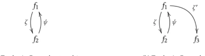
Example1 (Cyclic economy). There is a proportional transaction tax on all transfers of𝜆 = 10%.As depicted in Figure 2(a), there are two firms,𝑓1and𝑓2,which interact via two trades. The firms share the same utility function
𝑢𝑓𝑖(Ξ, 𝑡)=𝑣(Ξ) + Õ
𝜔∈Ω𝑓𝑖
e𝑡𝜔,
14Formally, we require thatΛ𝜔is continuous,Λ𝜔(0)=0,and𝑥2−Λ𝜔(𝑥2)<𝑥1−Λ𝜔(𝑥1)for all𝑥1>𝑥2>0.
15As Jagadeesan [2017] points out, our model cannot capture settings with imperfectly-insurable default risk in which firms partially finance purchases with trade credit and partially pay in cash.
16For example, firms might prefer one type of transfer over another if trades are priced in different currencies. The presence of multiple currencies with common exchange rates does not distort marketsper se. On the other hand, uninsurable risk or transaction costs associated with currency conversion can be modeled as variable transaction costs.
𝑓1
𝜁
𝑓2
𝜓
UU
(a) Trades in Examples 1 and 3.
𝑓1
𝜁
𝜁0
𝑓2
𝜓
UU
𝑓3 (b) Trades in Example 2.
Fig. 2. Trades in Examples 1, 2, and 3.Arrows point from sellers to buyers.
where the valuation𝑣is defined by
𝑣(∅)=0 𝑣({𝜁 , 𝜓})=10 𝑣({𝜁})=𝑣({𝜓})=−∞.
There are two sets of trades that can be supported in competitive equilibria: ∅ and{𝜁 , 𝜓}. For example, the arrangement[{𝜁 , 𝜓};𝑝]is a competitive equilibrium if−100 ≤ 𝑝𝜁 = 𝑝𝜓 ≤ 100,and the arrangement[∅;𝑝] is a competitive equilibrium if𝑝
𝜁 =𝑝
𝜓 ≥100 or𝑝
𝜁 =𝑝
𝜓 ≤ −100.17
Note that there are Pareto-comparable competitive equilibria: both𝑓1and𝑓2strictly prefer [{𝜁 , 𝜓};(0,0)]over any other competitive equilibrium with𝑝𝜁 =𝑝𝜓.As pointed out by Hart [1975], the existence of Pareto-comparable equilibria suggests that equilibria are constrained suboptimal.The competitive equilibria of the form[{𝜁 , 𝜓};𝑝]and [∅;𝑝]with𝑝𝜁 =𝑝𝜓≠0 are constrained Pareto-inefficient.
In contrast, by the First Welfare Theorem, competitive equilibria cannot be Pareto-comparable in economies without transaction taxes (see Supplementary Appendix F).
The second example shows that adding an outside option for𝑓1to Example 1 can shut down trade between𝑓1and𝑓2. The fact that enlarging the market can harm all firms suggests that equilibria are constrained suboptimal in the enlarged market [Hart, 1975]. The constrained suboptimality is due to pecuniary externalities. In the context of Examples 1 and 2, adding an outside option can cause prices to become extreme, inducing heavy trading losses (due to taxes) that shut down the market. In contrast, in economies without transaction taxes, adding an outside option can only affect which other trades are realized if the outside option is used in equilibrium (see Supplementary Appendix F).
Example2 (Cyclic economy with an outside trade). As depicted in Figure 2(b), there are three firms,𝑓1, 𝑓2,and𝑓3,which interact via three trades. The firms’ utility functions are
𝑢𝑓𝑖(Ξ, 𝑡)=𝑣𝑓𝑖(Ξ) + Õ
𝜔∈Ω𝑓𝑖
e𝑡𝜔,
17In general,[ {𝜁 , 𝜓};𝑝]is a competitive equilibrium if and only if
min{𝑝𝜁,0.9𝑝𝜁} +min{−𝑝𝜓,−0.9𝑝𝜓} ≥ −10 and min{−𝑝𝜁,−0.9𝑝𝜁} +min{𝑝𝜓,0.9𝑝𝜓} ≥ −10.
Similarly,[∅;𝑝]is a competitive equilibrium if and only if
min{𝑝𝜁,0.9𝑝𝜁} +min{−𝑝𝜓,−0.9𝑝𝜓} ≤ −10 and min{−𝑝𝜁,−0.9𝑝𝜁} +min{𝑝𝜓,0.9𝑝𝜓} ≤ −10.
where𝑣𝑓𝑖is the valuation of firm𝑓𝑖. We let𝑣𝑓𝑖(∅)=0 for all firms. Extending Example 1, firm𝑓1’s valuation is defined by
𝑣𝑓1({𝜁 , 𝜓})=𝑣𝑓1({𝜁0, 𝜓})=10 𝑣𝑓1({𝜁})=𝑣𝑓1({𝜁0})=𝑣𝑓1({𝜓})=−∞
𝑣𝑓1({𝜁 , 𝜁0})=𝑣𝑓1({𝜁 , 𝜁0, 𝜓})=−∞.
As in Example 1, firm𝑓2’s valuation is defined by
𝑣𝑓2({𝜁 , 𝜓})=10 𝑣𝑓2({𝜁})=𝑣𝑓2({𝜓})=−∞. Firm𝑓3’s valuation is defined by𝑣𝑓3({𝜁0})=300.
Trade𝜁0cannot be realized in equilibrium due to the technological constraints of𝑓1and𝑓2.Thus, we must have 𝑝𝜁0≥300 in any competitive equilibrium, as𝑓3must weakly prefer∅over{𝜁0}in equilibrium. For trade to occur,𝑓1 must prefer𝜁 over𝜁0,and so we must have𝑝𝜁 ≥300.With 10% taxation and𝑝𝜁 ≥300,at least $30 in taxes must be paid if𝜁is traded. But $30 exceeds the gains from trade between𝑓1and𝑓2,and so trade cannot occur in any competitive equilibrium. An example of a competitive equilibrium is[∅;𝑝],where𝑝𝜁 =𝑝𝜓 =𝑝𝜁0 =350.Thus, introducing an outside option that is not used can shut down a market when there are distortionary transaction taxes.18
4 EXISTENCE OF COMPETITIVE EQUILIBRIA
Due to the presence of indivisibilities, competitive equilibria need not exist in our model without further assumptions on preferences. Our key condition is full substitutability [Hatfield et al., 2013].19Intuitively, full substitutability requires that every firm views its upstream trades as gross substitutes for each other, its downstream trades as gross substitutes for each other, and its upstream and downstream trades as gross complements for one another.20
Assumption 1(Full substitutability—FS, Hatfield et al., 2013). For all𝑓 ∈𝐹and all finite sets of contracts𝑌 , 𝑌0⊆𝑋𝑓 with𝑌𝑓→⊆𝑌0
𝑓→and𝑌→𝑓 ⊇𝑌0
→𝑓,we have
𝑍0∩𝑌𝑓→⊆𝑍 and 𝑍∩𝑌0
→𝑓 ⊆𝑍0
if𝐶𝑓(𝑌)={𝑍}and𝐶𝑓(𝑌0)={𝑍0}.
Full substitutability requires that an expansion in the set of upstream (resp. downstream) options and a contraction in the set of downstream (resp. upstream) options only makes upstream (resp. downstream) contracts less attractive and downstream (resp. upstream) contracts more attractive for the firm. Technically, we impose this condition only on sets of contracts from which the firm’s utility-maximizing choice is unique. In Appendix B, we show that full substitutability is equivalent to a substitutability property that deals with indifferences more explicitly.21
18However, firms𝑓1and𝑓2trade𝜁and𝜓in every core outcome, and the core is non-empty. Indeed, the outside option does not disrupt trade in the core because𝑓1and𝑓3cannot form a core block without breaking offalltrade with𝑓2.
19Full substitutability generalizes gross substitutability [Gul and Stacchetti, 1999, Kelso and Crawford, 1982]. We use thechoice-language full substitutability condition introduced by Hatfield et al. [2013], which extends the same-side substitutability and cross-side complementarity conditions of Ostrovsky [2008] to choice correspondences.
20Section IIB in Hatfield et al. [2013] provides a detailed discussion of the full substitutability condition in the context of trading networks with transferable utility. For example, full substitutability rules out complementarities between inputs.
21Several of our proofs use the equivalence between our two definitions of full substitutability.
Hatfield et al. [2013] also need to assume that firms’ valuations of sets of trades are never+∞to ensure that competitive equilibria exist. We impose a similar condition that is adapted to settings in which utility is not perfectly transferable. Our condition requires that compensating variations of moving from autarky to trade are bounded below—i.e., that no set of trades is so desirable that it is preferred to autarky at any level of total transfers. This condition is satisfied in transferable utility economies when valuations are bounded above.
Assumption 2(Bounded compensating variations—BCV). For all𝑓 ∈𝐹 ,we have inf
𝑢𝑓(Ξ,𝑡) ≥0
Õ
𝜔∈Ω𝑓
𝑡𝜔>−∞.
BCV requires that net transfersÍ
𝜔∈Ω𝑓𝑡𝜔are bounded below over all transfer vectors𝑡that are acceptable alongside some set of tradesΞ.If a firm is willing to accept trades alongside arbitrary negative net transfers, then BCV fails. BCV is a weak assumption that is likely to be satisfied in any real-world economy. In particular, BCV is satisfied in Examples 1 and 2. Note that BCV allows for technological constraints, in that it permits sets of trades to be so undesirable to a firm that they remain worse than autarky regardless of how much the firm receives in transfers.
FS and BCV together ensure that competitive equilibria exist in trading networks. In Supplementary Appendix F, we show by example that competitive equilibria may not exist if BCV is not satisfied.
Theorem 1. Under FS and BCV, competitive equilibria exist.
To prove Theorem 1, we construct a modified economy by giving every firm options to execute all trades at a very undesirable price. Specifically, we give every firm the option to make any trade by paying a cost of
Π>−Õ
𝑓∈𝐹
inf
𝑢𝑓(Ξ,𝑡) ≥0
Õ
𝜔∈Ω𝑓
𝑡𝜔. (1)
The penaltyΠcan be chosen to be finite due to BCV. Hence, firms have bounded willingness to pay for any contract in the modified economy, in a sense that we make precise in Section 5.2.22 We discretize prices and use a generalized Deferred Acceptance algorithm [Fleiner et al., 2018b, Hatfield and Kominers, 2012, Ostrovsky, 2008] to show the existence of approximate equilibria in the modified economy. A limiting argument yields the existence of competitive equilibria in the modified economy, as in Crawford and Knoer [1981] and Kelso and Crawford [1982]. The fact thatΠis sufficiently large (i.e., (1) is satisfied) ensures that we actually obtain competitive equilibria in the original economy.23 5 RELATIONSHIPS BETWEEN COMPETITIVE EQUILIBRIA
AND COOPERATIVE SOLUTION CONCEPTS
We now study the relationships between competitive equilibria and cooperative solution concepts from matching theory. Instead of assuming that firms are price-takers, we allow firms to recontract while keeping or dropping existing contracts. We focus on two solution concepts: trail stability and stability.
A key ingredient of any reasonable stability property is individual rationality, which requires that no firm wants to drop any signed contract.
22Hatfield et al. [2013] apply a related, but not exactly analogous, transformation in the proof of their existence result (Theorem 1 in Hatfield et al. [2013]).
Specifically, Hatfield et al. [2013] give firms both the option to make a trade by paying a cost ofΠand the option to dispose of an undesired trade for a cost ofΠ(for a sufficiently largeΠ). The Hatfield et al. [2013] approach does not in general preserve full substitutability at the level of generality of our model.
23Theorem 1 generalizes Theorem 2 in Kelso and Crawford [1982] and Theorem 1 in Hatfield et al. [2013].
Definition 2(Hatfield et al., 2013, Roth, 1984). An outcome𝐴⊆𝑋 isindividually rationalif𝐴𝑓 ∈𝐶𝑓(𝐴𝑓)for all 𝑓 ∈𝐹.
5.1 Trail stability
Trail stability [Fleiner et al., 2018b] is a natural extension of pairwise stability (in the sense of Gale and Shapley [1962]) to trading networks. A trail is a sequence of contracts such that a buyer in one contract is a seller in the next contract.
A trail may involve a firm more than once and can begin and end with contracts that involve the same firm.
Definition 3. A sequence of contracts(𝑥1, . . . , 𝑥𝑛)is atrailifb(𝑥𝑖)=s(𝑥𝑖+1)for all 1≤𝑖≤𝑛−1.
Trail-stable outcomes are immune to sequential deviations called locally blocking trails. A locally blocking trail begins with a firm offering a sale that it wishes to sign given its existing contracts, possibly while dropping some existing contracts. The buyer may accept the offered contract while dropping some of his existing contracts, in which case a locally blocking trail is formed. The buyer may also hold the proposal and offer an additional sale to the original proposer or to another firm. This trail of linked offers continues until a firm accepts an offered contract without having to offer another sale, in which case a locally blocking trail is formed.24
Our formal definition of trail stability extends the definition given by Fleiner et al. [2018b] to settings with indiffer- ences.
Definition 4. A trail(𝑧1, . . . , 𝑧𝑛)locally blocksan outcome𝐴if:
• 𝐴𝑓
1∉𝐶𝑓1(𝐴𝑓
1∪ {𝑧1}),where𝑓1=s(𝑧1);
• 𝐴𝑓
𝑖+1∉𝐶𝑓𝑖+1(𝐴𝑓
𝑖+1∪ {𝑧𝑖, 𝑧𝑖+1})for 1≤𝑖≤𝑛−1,where𝑓𝑖+1=b(𝑧𝑖)=s(𝑧𝑖+1); and
• 𝐴𝑓
𝑛+1∉𝐶𝑓𝑛+1(𝐴𝑓
𝑛+1∪ {𝑧𝑛}),where𝑓𝑛+1=b(𝑧𝑛).
Such a trail is called alocally blocking trail. An outcome istrail-stableif it is individually rational and there is no locally blocking trail.
A trail locally blocks an individually rational outcome if, at every point at which a trail passes through a firm, the firm would like some of the contracts that are available to it locally in the trail (when given access to the existing contracts). Intuitively, one should think of contracts in a locally blocking trail as being proposed by telephone by a manager at one firm to a manager at another [Fleiner et al., 2018b]. If the sequence of phone conversations returns to a firm, a different manager (e.g., one from another division) picks up the phone and considers the latest offer. Her decisions are independent of the offers received and made by the first manager. Any manager’s unilateral decision to accept an offered contract completes a locally blocking trail.
5.2 A cooperative interpretation of competitive equilibria
The main result of this section provides a cooperative interpretation of competitive equilibrium that holds even in the presence of frictions.
Theorem 2. Every competitive equilibrium outcome is trail-stable.
Theorem 2 implies that price-taking firms cannot improve upon a market equilibrium by deviating along trails. In light of Theorem 2, any prediction of our model that holds in every trail-stable outcome must hold in every competitive equilibrium outcome.
24Note that locally blocking trails can also develop in the reverse direction, with firms offering to buy instead of to sell.
To see the intuition behind Theorem 2, consider any competitive equilibrium and any trail. In order for sellers to want to propose the contracts in the trail, the prices of all trades in the trail must be greater than their equilibrium prices.
But the last buyer will only accept an offer if the price in the last contract is lower than the equilibrium price of the corresponding trade. Hence, there cannot be any locally blocking trails. Theorem 2 does not require any assumptions beyond the monotonicity of utility in transfers. As we will show in Section 5.3, competitive equilibria do not satisfy stronger cooperative solution concepts in the presence of frictions.
In light of Theorem 2, the conclusions of Examples 1 and 2 hold for trail-stable outcomes as well. Thus, trail-stable outcomes can suffer from constrained suboptimality due to pecuniary externalities despite being defined cooperatively.25
Theorems 1 and 2 yield sufficient conditions for the existence of trail-stable outcomes.26 Corollary 1. Under FS and BCV, trail-stable outcomes exist.
5.3 Stability
Groups of firms might still be able to commit to recontracting at a trail-stable outcome. Stability rules out such recontracting opportunities, which are called blocks, and may be a more natural solution concept in settings in which firms can coordinate easily.27Hatfield et al. [2013] extend the definition of stability to settings with indifferences.
Definition 5(Hatfield et al., 2013). A non-empty set of contracts𝑍 ⊆ 𝑋 r𝐴blocks𝐴if, for all𝑓 ∈ 𝐹 and𝑌 ∈ 𝐶𝑓(𝐴𝑓 ∪𝑍𝑓),we have𝑍𝑓 ⊆𝑌. An outcome isstableif it is individually rational and unblocked.
In a stable outcome, no group of firms can commit to recontracting among themselves while being free to drop any contracts. Unfortunately, competitive equilibria may be unstable in the presence of frictions; moreover, stable outcomes need not even exist.28Hence, as Fleiner et al. [2018b] argue, stability may be too stringent of a solution concept in general networks.
Example2continued(Stable outcomes need not exist in the presence of frictions). There are no stable outcomes in Example 2. Indeed, note that the no-trade outcome is unstable, since it is blocked by trade between𝑓1and𝑓2. Note also that𝑓1and𝑓3cannot trade in any individually rational outcome due to the technological constraints faced by𝑓1and𝑓2. On the other hand, any individually rational outcome that involves trade between𝑓1and𝑓2is blocked by trade between𝑓1and𝑓3. Indeed, note that𝜁 cannot be traded at any price greater than $200 in an individually rational outcome, since the social surplus of trade between𝑓1and𝑓2is only $20 and making a transfer of at least $200 requires paying a transaction tax of at least $20. But the contract(𝜁0,250)blocks any outcome in which𝜁 is traded at price below $250.29
As noted by Hatfield and Kominers [2012], requiring that the trading network is acyclic—i.e., that it forms a vertical supply chain—helps restore the existence of stable outcomes in settings with discrete, bounded prices. Appendix A
25As shown by Blair [1988] and Klaus and Walzl [2009], (pairwise) stable outcomes can suffer from constrained suboptimality even in two-sided many-to-many matching markets.
26Corollary 1 is a version of Theorem 1 in Fleiner et al. [2018b]—which generalizes Theorem 1 in Ostrovsky [2008] from supply chains to general networks—for settings with prices that are continuous and potentially unbounded.
27See Roth [1984, 1985], Hatfield and Milgrom [2005], Echenique and Oviedo [2006], and Hatfield and Kominers [2012, 2017].
28Determining whether a stable outcome exists and determining whether a particular outcome is stable are both computationally intractable problems in trading networks with cycles and discrete contracts [Fleiner, Jankó, Schlotter, and Teytelboym, 2018a]. Trail stability is more natural from a computational perspective—trail-stable outcomes can be found in polynomial time using the generalized Deferred Acceptance algorithm under full substitutability [Fleiner et al., 2018b].
29An alternative proof can be given using one of our lifting results (Theorem 3). Indeed, note that the no-trade outcome is not stable. However, any stable outcome must lift to a competitive equilibrium by Theorem 3, and trade does not occur in any competitive equilibrium.
shows that similar logic carries over to our setting, which features unbounded, continuous prices. The underlying reason is that stability and trail stability coincide in acyclic networks, at least under FS, as we show in Appendix A.
Even in trading networks with cycles, under FS, stability actually refines trail stability.30 Proposition 1. Under FS, every stable outcome is trail-stable.
If FS is not satisfied, then stable outcomes may not be trail-stable (see Supplementary Appendix F).
5.4 Competitive interpretations of trail stability and stability
We now develop competitive interpretations of trail stability and stability. Formally, we say that an outcome𝐴lifts to a competitive equilibriumif𝐴is a competitive equilibrium outcome—that is, if𝐴can be supported by competitive equilibrium prices. As an outcome specifies prices for realized trades, the non-trivial part of lifting an outcome to a competitive equilibrium is finding equilibrium prices for unrealized trades.
Hatfield et al. [2013] show by example that stable outcomes do not generally lift to competitive equilibria when FS is not satisfied. Therefore, we maintain FS throughout this section. We first prove a positive result, namely that stable outcomes lift to competitive equilibria under the conditions for the existence of competitive equilibria.31
Theorem 3. Under FS and BCV, stable outcomes lift to competitive equilibria.
Frictions can cause stable outcomes to fail to exist in general networks as Example 2 shows. Therefore, for many trading networks with frictions, Theorem 3 has no bite. On the other hand, trail-stable outcomes need not lift to competitive equilibria even under FS and BCV, as the following example shows.
Example3 (Trail-stable outcomes need not lift to competitive equilibria under FS and BCV). As depicted in Figure 2(a), there are two firms,𝑓1and𝑓2,which interact via two trades. The firms share the same utility function
𝑢𝑓𝑖(Ξ, 𝑡)=𝑣(Ξ) + Õ
𝜔∈Ω
𝑡𝜔,
where𝑣is as in Example 1. The no-trade outcome is trail-stable but inefficient. However, as utility is transferable, all competitive equilibrium outcomes are efficient. In particular, the no-trade outcome cannot lift to a competitive equilibrium.
In Example 3, both firms face hard technological constraints: they are unwilling to execute any trade individually at any finite price, but would like to complete both trades together. The no-trade outcome is trail-stable because neither the buyer nor the seller is willing to offer to buy or sell a single trade at any finite price.
To ensure that trail-stable outcomes lift to a competitive equilibrium, we impose a different regularity condition than BCV. Intuitively, we require that firms have bounded willingness to pay for any trade.
Assumption 3(Bounded willingness to pay—BWP). There exists𝑀such that for all firms𝑓 ∈𝐹and all finite sets of contracts𝑌 , 𝑍 ⊆𝑋𝑓 with𝑍∈𝐶𝑓(𝑌):
• If(𝜔 , 𝑝𝜔) ∈𝑍→𝑓,then𝑝𝜔<𝑀.
30Proposition 1 is a version of Lemma 5 in Fleiner et al. [2018b] for settings with prices that are continuous and potentially unbounded.
31Theorem 3 generalizes Theorem 6 in Hatfield et al. [2013] to trading networks with distortionary frictions and income effects. Stable outcomes exist in acyclic networks even in the presence of frictions, as we show in Appendix A.
• If(𝜔 , 𝑝𝜔) ∈𝑍𝑓→,then𝑝𝜔>−𝑀.
BWP requires that no firm is willing to pay more than𝑀for any trade—i.e., no firm is willing to buy any trade at a price more than𝑀or sell any trade at a price less than−𝑀. BWP rules out certain technological constraints, including those that are permitted under BCV and by Hatfield et al. [2013]. In particular, BWP does not allow a firm to require a particular input in order to produce a particular output, as such constraints make a firm willing to pay arbitrarily high prices for the input if the firm is able to procure arbitrarily high prices for the output. However, BWP allows for capacity constraints, since they never make trades desirable at extremely unfavorable prices.
BWP helps ensure that trail-stable outcome lift to competitive equilibria.32 Theorem 4. Under FS and BWP, trail-stable outcomes lift to competitive equilibria.
Theorem 4 provides a competitive interpretation of trail stability: any trail-stable outcome is consistent with price- taking equilibrium behavior by all firms (at least under FS and BWP). In light of Theorem 4, any prediction of our model that holds in every competitive equilibrium must hold in every trail-stable outcome.
Theorems 2 and 4 imply that competitive equilibria are essentially equivalent to trail-stable outcomes in our model.33 Corollary 2. Under FS and BWP, competitive equilibrium outcomes and trail-stable outcomes exist and coincide.
Corollary 2 provides competitive foundations for trail stability and cooperative foundations for competitive equilib- rium: the assumption that firms coordinate on a trail-stable outcome (as in a thin market) produces the same predictions as the assumption that firms take prices in equilibrium (as in a thick market). Therefore, equilibrium analysis can be performed using scale-independent solution concepts, even in markets with frictions.
6 COMPLETE MARKETS
Trail-stable and competitive equilibrium outcomes might be constrained Pareto-inefficient in the presence of proportional transaction taxes or other distortionary frictions (see Examples 1 and 2). In the presence of transaction taxes, for example, all firms find reductions in outgoing payments more desirable than equal increases in incoming payments. As a result, firms have different marginal rates of substitution between forms of transfer, unlike in settings with complete financial markets.
Since we do not explicitly model financial markets, we formalize “equalization of marginal rates of substitution between forms of transfer" as “indifference between all forms of transfer" in defining our market completeness condition.
Intuitively, if the firms share the same marginal rates of substitution between forms of transfer, then transfers can be redenominated so that the marginal rates of substitution become 1. The possibility of redenomination is precisely why, for example, the presence of multiple currencies does not cause market incompletenessper se.
Assumption 4(Complete markets—CM). For all𝑓 ∈ 𝐹 and𝑡 , 𝑡0 ∈ RΩ𝑓 withÍ
𝜔∈Ω𝑓
𝑡𝜔 = Í
𝜔∈Ω𝑓
𝑡𝜔0,we have 𝑢𝑓(Ξ, 𝑡)=𝑢𝑓(Ξ, 𝑡0)for allΞ⊆Ω𝑓.
Recall that, in Examples 1 and 2, paying one unit is more costly for firms than receiving one unit (due to transaction taxes). Assumption CM rules out these differences in the costs of transfers and requires that firms only care about the
32Despite the fact that BWP is not satisfied in Examples 1 and 2, trail-stable outcomes lift to competitive equilibria in both examples. Thus, BWP is sufficient but not necessary for trail-stable outcomes to lift to competitive equilibria.
33To derive Corollary 2 formally, we need to establish that competitive equilibria exist under FS and BWP, as Theorem D.1 in the Supplementary Appendix shows.
total transfers that they receive or pay. Therefore, CM requires that a unit of transfer for one trade be equivalent to a unit of transfer for any other trade.34Under CM, we can write𝑢𝑓(Ξ, 𝑡)=𝑢𝑓(Ξ, 𝑞),where𝑞=Í
𝜔∈Ω𝑡𝜔is the total or net transfer. Note that while CM rules out distortionary frictions—such as variable sales taxes, bargaining costs, and incompleteness in financial markets—fixed transaction costs and income effects are still permitted under CM.35
We begin our analysis of trading networks with complete markets by recalling the definition of strong group stability, which is the most stringent stability property from the literature on matching with contracts. A strongly group stable outcome is immune to blocks by coalitions of firms that can commit to better, new contracts and maintain any existing contracts with each other and with firms outside the blocking coalition.
Definition 6(Hatfield et al., 2013). An outcome𝐴isstrongly unblockedif there do not exist a non-empty set𝑍 ⊆𝑋r𝐴 and sets of contracts𝑌𝑓 ⊆𝐴𝑓 ∪𝑍𝑓 for𝑓 ∈𝐹such that𝑌𝑓 ⊇𝑍𝑓 and𝑈𝑓
𝑌𝑓
>𝑈𝑓
𝐴𝑓
for all𝑓 ∈𝐹with𝑍𝑓 ≠∅. An outcome isstrongly group stableif it is individually rational and strongly unblocked.
In Definition 6,𝑌𝑓 is the set of contracts that𝑓 signs in the block. Note that𝑌𝑓 need not be𝑓’s best choice from the set of available contracts. In particular, strong group stability rules out blocks in which firms only improve their utility by selecting all of the blocking contracts. Hence, as Hatfield et al. [2013] show, strong group stability is stronger than stability. Moreover,𝑌𝑓 can contain existing contracts that the counterparties no longer want. In particular, strong group stability rules out blocks in which different members of the blocking coalition can make selections from the set of existing contracts that are incompatible with one another or involve firms outside the coalition. Hence, strong group stability also refines properties such as (strong) setwise stability [Echenique and Oviedo, 2006, Klaus and Walzl, 2009]
and the core.36
It appears extremely unlikely that firms would rationally deviate from a strongly group stable outcome, and competitive equilibria are strongly group stable in complete markets.37
Theorem 5(First Welfare Theorem). Under CM, competitive equilibrium outcomes are strongly group stable.
Since strongly group stable outcomes are stable and in the core, Theorem 5 implies that competitive equilibrium outcomes are stable and in the core in complete markets. As core outcomes are Pareto-efficient, Theorem 5 is a version of the First Welfare Theorem [Debreu, 1951].
Combining Theorem 5 with our results on markets with frictions, we obtain that all of the solution concepts described in this paper are essentially equivalent in complete markets (under FS and BWP).
Corollary 3. Under FS, BWP, and CM, competitive equilibrium outcomes, strongly group stable outcomes, stable outcomes, and trail-stable outcomes exist and coincide.
When markets are complete, we can also restate BCV more simply using only total transfers, since firms are indifferent regarding the sources of transfers.
34In particular, any transferable utility economy satisfies CM.
35When assumed jointly, FS and CM restrict income effects for certain agents. In particular, intermediaries that buy or sell more than one trade cannot experience income effects. However, firms that act only as buyers or only as sellers can experience limited income effects. Moreover, firms that buy or sell only one trade at a time can experience arbitrary income effects. In incomplete markets, on the other hand, all firms can experience income effects even under FS.
36As pointed out by Hatfield et al. [2013], strong group stability also refines strong stability [Hatfield and Kominers, 2015], and group stability [Konishi and Ünver, 2006].
37Theorem 5 extends Theorem 5 in Hatfield et al. [2013], which shows that competitive equilibrium outcomes are strongly group stable, to settings with income effects or risk aversion.