Proactive Minimization of Convolutional Networks

(1)

Proactive Minimization of Convolutional Networks

Bendeg´uz Jenei Institute of Informatics

University of Szeged Jenei.Bendeguz@stud.u-szeged.hu

G´abor Berend Institute of Informatics

University of Szeged MTA-SZTE

Research Group on Artificial Intelligence berendg@inf.u-szeged.hu

L´aszl´o Varga Institute of Informatics

University of Szeged vargalg@inf.u-szeged.hu

Abstract—Optimizing the performance of convolutional neural networks (CNNs) in real applications (i.e., production programs) is crucial. The desired network can perform a task while having minimal evaluation time and resource requirement. The evaluation time of a network strongly depends on the number of layers and the number of convolutional kernels in each layers.

Therefore, by minimizing the network while keeping its accuracy high is a frequent task. In this paper, we present variations of a method for the automatic minimization of convolutional networks. Our method minimizes the neural network by omitting convolutional kernels during the training process, while also keeping the quality of the results high.

Index Terms—Deep Learning, Convolutional Networks, Auto- matic Scaling

I. INTRODUCTION

The benefits of using properly sized neural networks in- clude portability and resource efficiency. With less demanding networks, cheaper hardware such as mobile devices will be capable of running convolutional networks, making them more widely available. The computational costs can also be reduced, producing results faster and with more modest hardware.

Classical approach for determining the optimal network structure is a trial-by-error strategy trying out various networks structures and choosing one giving acceptably good results with the minimal computational cost. Another, more automatic method for finding optimal network structure is using grid search, i.e., training multiple networks with varying number of neurons in each layer. The above processes, however, can be long and time consuming, since training networks from scratch can be resource demanding, and/or require human interaction.

In this paper, we propose automatic ways of determining the appropriate neuron count and network size for a given problem. This way, no repeated testing and trial-and-error is required for finding proper hyperparameters of the network.

The other advantage of our proposed solution is that the minimization process works automatically without requiring human intervention. This approach is also less resource demanding in contrast to more resource intensive solutions,

This research was in part supported by the project ”Integrated program for training new generation of scientists in the fields of computer science”, no EFOP-3.6.3-VEKOP-16-2017-0002. The project has been supported by the European Union and co-funded by the European Social Fund. This work was in part supported by the National Research, Development and Innovation Office of Hungary through the Artificial Intelligence National Excellence Program (grant no.: 2018-1.2.1-NKP-2018-00008).

such as the grid search, i.e., training multiple networks with different numbers of neurons in each layer.

The method described in this paper tries to proactively de- termine the size of the network, by measuring its performance in the training process repeatedly and removing neurons based on various strategies. This is done by minimizing a network of initially bigger size. Then – with an appropriate selection strategy – we select a neuron to omit in the training process and checking if the network performance can be restored without the selected neuron. If good network performance can be obtained without the selected neuron, then we permanently remove it from the structure, and iteratively repeat the selection-reduction cycle.

We designed a test environment for testing neuron selection strategies for the minimization, and propose thee strategies for it. We also designed a process for the automatic minimization of networks, and evaluated the process under various condi- tions with a great number of software tests, by minimizing a fully convolutional neural network trained for edge detection.

II. RELATED WORK

CNNs have a prevalent presence in computer vision research [1]–[3]. Dropout [4] is a popular approach to increase the generalization ability of neural networks. By temporarily deactivating neurons with a predefined probability, it has the property to mitigate overfitting by preventing the assignment of excessive credit to a single neuron. Dropout essentially can be viewed as training an ensemble of classifiers at a time in an efficient manner [5], however, it does not remove neurons permanently from the network. Dropout is typically applied for fully connected layers in neural networks, but they are applicable for convolutional layers as well.

Our solution resembles dropout in that it essentially de- activates specific kernels of the CNN. A major distinction compared to drouput is nonetheless that instead of doing the deactivation in a stochastic manner and for a single batch, we deactivate kernels for multiple batches and might as well decide to discard them for the rest of the training and inference time.

Zhou et al. [6] performed ablation experiments by turning off individual units in CNNs. The main motivation in [6], however, was not to decrease the computational needs of the CNN architecture employed, but to gain insights about how IJCNN 2019 - International Joint Conference on Neural Networks, Budapest Hungary, 14-19 July 2019

(2)

specific kernels of CNNs specialize for the detection of certain object categories. In our work, we perform deactivation of convolution kernels in order to gain smaller – hence less resource intensive – networks without a substantial loss in performance for the task of edge detection.

Minimizing the complexity of neural networks has been in the focus of multiple previous research efforts [7]–[9].

[7] proposed a general approach for simplifying the model complexity of neural networks according to the minimum description length principle with their main goal not being to reduce the number of neurons, rather to minimize overall model complexity. The algorithm described in [8] specifi- cally deals with the enhancement of CNN architectures. The proposed approach is orthogonal to ours, as the main goal in [8] was not to decrease the size of a CNN, but rather to decrease the computational workload necessary for an unmodified CNN without relying on hardware acceleration. By analyzing the linear algebraic properties of the computations in CNNs, the algorithm proposed in [8] was capable of reducing computational requirements up to 47% without a serious loss in accuracy.

Molchanov et al. [9] introduced a CNN pruning framework similar to ours in a transfer learning setting. [9] relied on the large pre-trained networks, i.e., VGG-16 [3] and AlexNet [1], that they iteratively pruned and fine-tuned for image recognition and hand gesture recognition. Our framework differs from theirs in that we do not rely on pre-trained networks and our evaluation is focused on edge detection.

[10] proposed the minimization of neural networks by first training a high accuracy neural network and distilling its knowledge by a smaller student network which tries to mimic the behavior of the large teacher network. This approach nonetheless requires training multiple neural nets. Polino et al. proposes the joint usage of model distillation and quantization in order to increase model compression [11]. The recent work of [12] proposes a redundancy-aware in-training pruning strategy which builds upon the partitioning of the model.

This redundancy-aware approach operates on a magnitude- based strategy, i.e. weights below a certain threshold were pruned. This is different from our approach we disable entire convolutional kernels instead of single weights, furthermore, our criterion for pruning kernels is not magnitude-based.

III. EXPERIMENTALSETUP

For the development of the methods we designed an ex- perimental framework. This included a task for training the network, a test data set and various metrics for developing and evaluating automatic network minimization techniques.

We implemented our framework in Tesorflow [13].

We decided to use a simple image processing task to train the network for, namely we aimed at training a fully convolutional neural network which is capable of reproducing the output of the Canny edge detector [14] for any given input image. Although the Canny edge detector involves a sequence of complex steps, the network mimicking its behavior does not have to be too complex, which makes the design of the

methods easier and enables us to perform a large number of evaluations.

One should note, that the provided method can be extended for any types of neural networks (e.g., classification networks, RCNN-s, etc.) containing convolutional or fully connected layers. One only have to implement the removal of the computational units (i.e., convolutional kernels, or perceptrons) from the network.

A. Input data

The input data was gained from two sources. The input for training and validating the edge detection network was given by the Visual Object Classes Challenge 2012 (VOC2012) data set [15]. The VOC data set contains colored pictures with various objects of interest (including classes for airplanes, people, bicycles, horses, etc.) As our task was to perform edge detection, we did not rely on the labels of the images during training, solely the images themselves. For testing the final results, we used the test image set of the 2017 MS COCO database [16].

We cropped each image to the same size of256×256pixels and used the centre of the original image. Images with a size smaller then 256 pixels in any dimensions were padded with zeros.

The input of the networks had only one color channel, therefore, RGB images were converted to grey scale. The expected outputs were the results of the Canny edge detector, which we generated by the built-in Canny function of MATLAB.

We partitioned the data set to three parts. The training data was given by 10000 images of the VOC2012 data set. Another 100 images from the VOC2012 was used for validation of the nets. Finally, to get a sound final evaluation, we tested the accuracy on the 2017 MS COCO database containing 40670 images.

IV. METHODS

The starting point of the optimization is a maximal neural network. We start by determining a maximal networks structure that we assume is capable of learning the task at hand.

Then, pruning of the maximal network is performed in a two-stage procedure:

• First, train the maximal network until convergence,

• Then proactively omit convolutional kernels by removing them from the network until no more kernels can be removed while keeping the quality of the results within a tolerance limit.

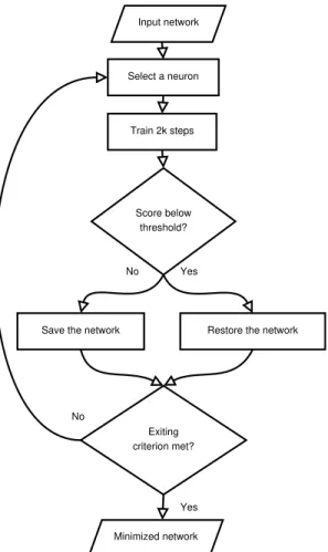
The iterative network minimization process uses a backtracking process, together with various neuron selection strategies that is illustrated in Figure 1.

The backtracking process includes saving the current stage of the network. Then, we select a convolutional kernel that we want to omit, and remove it from the network. The reduced network might have worse performance, therefore, we fine- tune the net by performing a limited number of training steps to gain back the accuracy of the results. Finally, we check if the results have approximately the same accuracy.

(3)

Exiting criterion met?

Train 2k steps

Score below threshold?

Select a neuron

Restore the network Yes

Yes No

Save the network No

Input network

Minimized network

Fig. 1. Process of the network optimization method.

We accept the new networks structure if the new accuracy is above an adaptive threshold value determined as a function of the previous evaluation of the model. If the accuracy of the imputed network is below the predefined tolerance level, we reject the last pruning step on the network and revert it to its previous state.

This process has a handful of parameters that we describe next. First of all, we need to have a neuron selection strategy to choose which convolutional kernel to omit. We detail various selection methods we considered in Section IV-A.

We also need to define a proper threshold for the tolerance level based on which we decide on the acceptance or the rever- sion of the change in the network structure. For this purpose we compared the_oldprevious accuracy of the network on the validation data set and compared it to the_newnew accuracy.

We kept the change if

new≥τ·old , (1) for some τ ∈ [0,1] threshold value. We employed different stopping criteria for our network reduction approach in con- junction with the different neuron filtering strategies.

Based on preliminary experiments we used a network containing three convolutional layers each followed by a ReLU activation. The kernels of each convolutional layer had the

Fig. 2. Illustration of the maximal network.

size of5×5×[input channel count]. The first two layers had 5 kernels, while the final layer had only one output, i.e., the predicted edge map. This network structure is illustrated in Figure 1.

We trained the network with the Adam optimizer [17]

minimizing the loss function

1−E(M,Mˆ) , (2)

where

E(M,Mˆ) = 2P(M,Mˆ)

2P(M,Mˆ) +N(M,Mˆ) , (3) having

P(M,Mˆ) =X

M∗Mˆ (4)

and

N(M,Mˆ) =X

|M −Mˆ| . (5) Here, we assume, thatM is the output of the neural network andMˆ is the expected edge map. Note that in the binary case, (3) is equivalent to the standard f1 measure often employed in information retrieval [18].

The training of the initial networks was performed with a batch size of 3 images, using10000 iterations.

A. Neuron Selection Strategies for the Reduction

We used various strategies for selecting the neuron to omit.

In this Section we summarize our findings.

1) Sequential Neuron Selection: The first selection strategy is a simple sequential method. When applying this approach we omitted all the neurons in a sequence one after the other.

We started with the first kernel of the first layer (i.e., the layer connected directly to the input) and omitted one neuron at a time.

(4)

After removing the current neuron, we trained the network for 2000 iterations and checked if the performance of the new net fulfilled the condition in (1). In case the condition is not met, we reverted the net to its previous checkpoint. If the threshold condition was fulfilled we accepted the change. No matter if the pruning was accepted or rejected, the algorithm continued with probing the next neuron in the sequence. The stopping criteria for this selection method was checking all the possible neurons.

2) Random Neuron Selection: We also evaluated a random strategy, where kernels to be omitted were selected randomly.

After removing and training the net further, we again checked if the new net can be accepted according to condition (1). This approach was allowed to propose kernel removals at most 50 times (including accepted and rejected proposals as well).

3) Selection Based on Cosine Similarity: Our assumption was that reduction is possible if the network contains redundancy in the kernels, i.e., some kernels perform very similar operations.

In order to reduce redundancy and network size simul- taneously, we designed a selection strategy based on the cosine similarity. Before each reduction step, we calculated the cosine similarities between the kernels of the same layers. The similarity was calculated by comparing vectors gained from the weights of the kernel together with the bias of the neuron.

This gave us similarity matrices showing the correspondence between kernels.

With the similarity matrices at hand, we still needed a numerical tool for comparing the kernels with one single number. Therefore, we calculated statistics for each kernel by the following tools:

• Average similarity with other neurons (Avg);

• Standard deviation of cosine similarities (Std);

• Maximal similarity with other neurons (Max);

• Minimal similarity with other neurons (Min);

• Median of cosine similarities with other neurons (Med).

To find out witch of the above metrics can be used for selecting the neuron to omit, we designed a set of experiments, where we calculated the statistics of neurons, and also tested the performance of the nets after removing the neuron.

We calculated the accuracy of the network directly after disabling a particular neuron and after training the net for 10000iterations. Then, we compared the final accuracy of the results to the statistics gained from the cosine similarities with three correlation coefficients.

As a convolutional kernel can hold the same information as another one by using an inverse kernel, we calculated statistics for the original and the absolute values of the cosine similarities as well.

We used one hundred networks trained from different random seeds to grain a reliable result. We calculated the correlations within each layers of the networks, and examined the average values of the results. The summary of our results can be found in Table I.

TABLE I

CORRELATIONS BETWEEN NETWORK ACCURACY AFTER DISABLING A NEURON COMPARED TO THE STATISTICS ON THE COSINE SIMILARITY. LOSS DENOTES THEf1SCORE AFTER OMITTING THE NET;BEST DENOTES

CORRELATION WITH THE BEST PERFORMANCE AFTER FURTHER TRAINING. TABLES SHOW THREE CORRELATION COEFFICIENTS: PEARSON

(PRS); KENDALL(KND)ANDSPEARMAN(SPR).THE TWO TABLES SHOW STATISTICS USING THE SIGNED AND ABSOLUTE COSINE SIMILARITY AS

WELL. Signed Cosine Similarity

Avg Std Max Min Med

loss(prs) 0.21 0.26 0.06 -0.32 -0.20 loss(knd) 0.02 0.20 0.13 -0.30 -0.01 loss(spr) 0.04 0.28 0.21 -0.27 -0.02 best(prs) 0.11 0.14 0.15 -0.05 0.13 best(knd) 0.09 0.08 0.09 -0.04 0.09 best(spr) 0.13 0.12 0.14 -0.06 0.14

Absolute Cosine Similarity

Avg Std Max Min Med

loss(prs) 0.30 0.26 0.30 0.15 0.28 loss(knd) 0.18 0.16 0.19 0.08 0.16 loss(spr) 0.24 0.22 0.26 0.11 0.22 best(prs) 0.04 0.05 0.06 0.02 0.03 best(knd) 0.03 0.04 0.05 -0.01 0.02 best(spr) 0.04 0.06 0.07 -0.01 0.02

TABLE II

STATISTICS SHOWING THE PERFORMANCE OF NETWORKS BEFORE AND AFTER DISABLING ONE NEURON BASED ON COSINE SIMILARITY. RESULTS

ARE GIVEN FOR ONLY DISABLING THE NEURON WITH A MAXIMAL VALUE OF THE ONE SPECIFIED CHARACTERISTICS(I.E., AVERAGE; STANDARD

DEVIATION; MAXIMUM; MINIMUM;MEDIAN)OF COSINE SIMILARITY WITHIN ITS LAYER,WITHOUT FURTHER TRAINING. THE TABLE ALSO SHOWS STATISTICS CORRESPONDING TO DISABLING EACH NEURON.

Before After After/Before Ratio Cos-Avg

0.7

0.467 0.667

Cos-Std 0.617 0.881

Cos-Max 0.584 0.835

Cos-Min 0.481 0.687

Cos-Med 0.516 0.736

Any neuron 0.549 0.784

According to the results, immediately after omitting a neuron there are week correlations between the statistics of the cosine similarity and the performance of the new network.

In case of the signed correlations, the strongest correlation is with the minima of the cosine similarities, which is an inverse correlation. This indicates that choosing the net with the minimal cosine similarity will result in the best output.

We observed somewhat strong positive correlations for the standard deviation, which means that our networks relied less on the neurons with big deviation in cosine similarity. These phenomena are quite counter-intuitive, hence, worth a deeper examination which can be subject to later research.

We also found that omitting neurons in the networks leads to major drops in the accuracy and concluded that further training with the modified network is necessary. (Related statistics can be seen in Table II.) Therefore, we decided to choose a strategy based on the best result after refinement training.

Based on Table I we found that the signed cosine similarity is the best for the neuron selection. We found the strongest correlation with the maxima of the cosine similarities, indi-

(5)

TABLE III

STATISTICS SHOWING THE PERFORMANCE OF NETWORKS BEFORE,AND AFTER DISABLING ONE NEURON BASED ON COSINE SIMILARITY AND

FURTHER TRAINING THE NET TO REGAIN ACCURACY. RESULTS ARE GIVEN FOR ONLY DISABLING THE NEURON WITH A MAXIMAL VALUE OF

THE ONE SPECIFIED CHARACTERISTICS(I.E., AVERAGE; STANDARD DEVIATION; MINIMUM; MAXIMUM;MEDIAN)OF COSINE SIMILARITY

WITHIN ITS LAYER,WITHOUT FURTHER TRAINING. THE TABLE ALSO SHOWS STATISTICS CORRESPONDING TO DISABLING EACH NEURON.

Before Refined Refined/Before Ratio Cos-Avg

0.7

0.710 1.013

Cos-Std 0.710 1.013

Cos-Max 0.710 1.013

Cos-Min 0.710 1.014

Cos-Med 0.710 1.014

Any neuron 0.709 1.026

cating that after omitting the neuron with the highest maximal similarity, the network can be refined to high accuracy. In many cases, this meant that the new net was closely as good – or in some cases even better then – the one before (see Table III).

This phenomena is understandable, since kernels with high cosine similarities are similar to other kernels performing similar tasks. This is redundancy in the network and by reducing redundancy, the performance can be restored.

We also used this set of experiments for finding the optimal parameters of the network minimization process. We found that – on average – after removing a neuron the further training need approximately 500 iterations to converge. Hence, running 2000 iterations described in Section IV-A1 is sufficient to regain maximal performance.

The net reduction method composed of this approach is based on removing the neuron with the highest cosine similarity. Again, if the accuracy cannot be restored after a given amount of iterations, we revert the net to the checkpoint prior to the removal of the given neuron. In this case, we also try to remove the neuron with the second biggest cosine similarity, and finally the third one. We repeat this process until the third try in a sequence does not result in a successful removal, or we reach a limit of 20 tries.

V. RESULTS AND DISCUSSION

We performed experiments by training the networks described above and minimizing them by the proposed minimization approaches. We compared three basic approaches:

• The sequential method trying to remove all the neurons (later referenced as Sequential);

• Removal of 50 randomly selected neurons (denoted as Random50);

• And the maximal cosine similarity-based approach with 20 tries (denoted as CosMax).

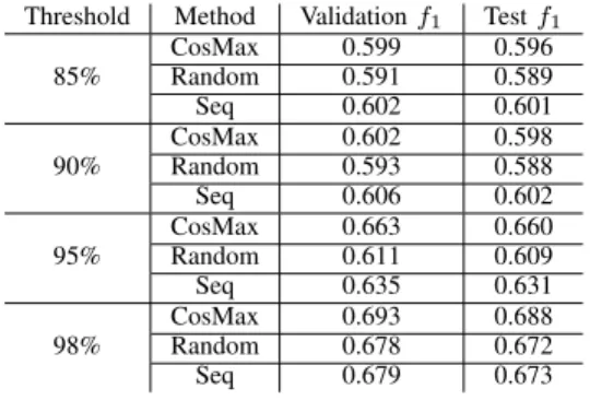
We evaluated the networks in four sets of test cases. In the first case, the acceptance threshold in (1) was set toτ= 0.85, and in the further cases it was set to 0.90,0.95 and0.98. In each case, we ran the training and minimization 50 times to grain statistically solid results.

TABLE IV

STATISTICS SHOWING THE PERFORMANCE OF NETWORKS BEFORE,AND AFTER DISABLING ONE NEURON BASED COSINE SIMILARITY. RESULTS ARE GIVEN FOR ONLY DISABLING THE NEURON WITH A MAXIMAL VALUE

OF THE ONE SPECIFIED CHARACTERISTICS(I.E., AVERAGE; STANDARD DEVIATION; MINIMUM; MAXIMUM;MEDIAN)OF COSINE SIMILARITY WITHIN ITS LAYER,WITHOUT FURTHER TRAINING. TABLE ALSO SHOWS

STATISTICS CORRESPONDING TO THE DISABLING EACH NEURON. Threshold Method Validationf1 Testf1

85%

CosMax 0.599 0.596

Random 0.591 0.589

Seq 0.602 0.601

90%

CosMax 0.602 0.598

Random 0.593 0.588

Seq 0.606 0.602

95%

CosMax 0.663 0.660

Random 0.611 0.609

Seq 0.635 0.631

98%

CosMax 0.693 0.688

Random 0.678 0.672

Seq 0.679 0.673

We evaluated the networks with two considerations in mind. First, we wanted to see how successful the reduction strategies were in removing kernels. Therefore, we calculated the average number of removed neurons for the methods. This can be seen in Figure 3.

Second, we must note, that a reduced network is not worth a lot if its accuracy is greatly degraded. Therefore, we calculated the average drop of accuracy for the methods. This is summarized in Figure 4. We calculated these statistics by the average of thef1 score, in percent relative to thef1score of the first non-reduced network. We also calculated statistics comparing the validation and test evaluations, which can be found in Table IV.

Overall, we can say that the most (around 8) neurons were discarded for low tolerance thresholds, i.e., when using τ = 0.85 andτ= 0.9. In turn, the low threshold value forτ resulted in a drop in f1 score around 10%. We can say that by sacrificing a great portion of accuracy, we can significantly reduce the network.

On the other hand, by increasing the acceptance threshold – i.e., forcing the nets to re-gain most of their accuracy after removing a neuron – we can maintain good performance while keeping most of the neurons.

Using a high acceptance threshold τ, we found that the sequential and random methods performed better, than the CosM ax. They were able to omit 4-7 neurons (in the case ofτ = 0.98andτ= 0.95, respectively), compared to the 2-4 neurons disabled by the CosM ax. This was again in turn of a higher drop in the accuracy.

With the highest acceptance threshold, however, the Ran- dom a Seq methods were able to disable 4 more neurons, while still maintaining a high accuracy (i.e., only a 2% drop was observed).

Our results revealed that the random and sequential neuron removal strategies performed better compared to theCosM ax strategy as they removed more neurons, or the same amount of neurons with a smaller drop in accuracy.

(6)

85 90 95 98

Cos Max 8,00 7,88 3,98 1,90

Random 8,00 8,00 7,24 4,30

Seq 8,00 7,92 6,14 4,26

8,00 7,88

3,98

1,90

8,00 8,00

7,24

4,30

8,00 7,92

6,14

4,26

0,00 1,00 2,00 3,00 4,00 5,00 6,00 7,00 8,00 9,00

Fig. 3. Number of average removed neurons by the different network reduction strategies.

85 90 95 98

Cos Max 10,366% 9,841% 3,556% 0,753%

Random 11,179% 10,802% 8,818% 2,286%

Seq 10,095% 9,462% 6,394% 2,203%

10,4%

9,8%

3,6%

0,8%

11,2% 10,8%

8,8%

2,3%

10,095%

9,462%

6,394%

2,203%

0,00%

2,00%

4,00%

6,00%

8,00%

10,00%

12,00%

Fig. 4. Average drop inf1 score after the neuron removal process relative to thef1 score before removal.

Concerning the computational costs of the process, we can say that training one network in our experiments took 40,000 iterations (10,000 for the initial training and 3×5×2000 for the reduction attempts) with the iterative approach; less then 50,000 iterations for the CosM axstrategy and 110,000 iterations for the Random50 strategy. With the grid search strategy training networks for 10,000 iterations would have taken 150,000 iterations, giving a substantially longer training time.

According to our results, using the Sequential and Random50 strategies with a high τ = 0.95 or τ = 0.98 acceptance threshold can be useful for minimizing networks.

The Seq method seems to be a bit better as it has the advantage of having a lower iteration count thanRandom50.

The CosM ax strategy, on the other hand has the possibility of terminating even earlier performing informed removals, therefore it might minimize the network in less steps than the other strategies.

VI. CONCLUSION ANDFURTHERWORK

We proposed an algorithmic framework for the proactive minimization of convolutional networks and provided three strategies for iterative removal of neurons from a convolutional network. We evaluated the proposed methods to train and minimize a network for edge detection.

We found that the proposed methods were capable of automatically reduce the size of the initial networks by 26%

in our tests without a significant degradation in the network performance in trying to replicate the behavior of a Canny edge detector.

The proposed methods are faster than the traditional trial- and-error strategies for finding optimal network structures, as it does not need long processes of training networks of different structures from scratch. As opposed to the repeated training of the network with different size, we proposed to train one single network and fine-tune it in an effective manner.

We must emphasize that our findings can be generalized to other tasks and networks structures as well. The proposed

(7)

methods can be used for pruning any type on network that has removable computational units (i.e., convolution kernels, or perceptrons). In the future we are extending the studies to other types of networks, e.g., classification nets, RCNNs, and larger fully convolutional nets. Previous work on minimizing CNNs has focused on image classification rather than edge detection. As such, we are planning to adapt existing network pruning strategies for edge detection and empirically compare them to the method proposed in this paper.

REFERENCES

[1] K. He, X. Zhang, S. Ren, and J. Sun, “Deep residual learning for image recognition,” in2016 IEEE Conference on Computer Vision and Pattern Recognition, CVPR 2016, Las Vegas, NV, USA, June 27-30, 2016, pp. 770–778, 2016.

[2] S. Ren, K. He, R. B. Girshick, and J. Sun, “Faster r-cnn: Towards real-time object detection with region proposal networks.,” in NIPS (C. Cortes, N. D. Lawrence, D. D. Lee, M. Sugiyama, and R. Garnett, eds.), pp. 91–99, 2015.

[3] K. Simonyan and A. Zisserman, “Very deep convolutional networks for large-scale image recognition,” inInternational Conference on Learning Representations, 2015.

[4] N. Srivastava, G. Hinton, A. Krizhevsky, I. Sutskever, and R. Salakhut- dinov, “Dropout: A simple way to prevent neural networks from overfitting,”J. Mach. Learn. Res., vol. 15, pp. 1929–1958, Jan. 2014.

[5] K. Hara, D. Saitoh, and H. Shouno, “Analysis of dropout learning regarded as ensemble learning,” inInternational Conference on Artificial Neural Networks, pp. 72–79, Springer, 2016.

[6] B. Zhou, Y. Sun, D. Bau, and A. Torralba, “Revisiting the importance of individual units in cnns via ablation,”CoRR, vol. abs/1806.02891, 2018.

[7] G. E. Hinton and D. van Camp, “Keeping the neural networks simple by minimizing the description length of the weights,” inProceedings of the Sixth Annual Conference on Computational Learning Theory, COLT

’93, (New York, NY, USA), pp. 5–13, ACM, 1993.

[8] J. Cong and B. Xiao, “Minimizing computation in convolutional neural networks.,” inICANN (S. Wermter, C. Weber, W. Duch, T. Honkela, P. D. Koprinkova-Hristova, S. Magg, G. Palm, and A. E. P. Villa, eds.), vol. 8681 ofLecture Notes in Computer Science, pp. 281–290, Springer, 2014.

[9] P. Molchanov, S. Tyree, T. Karras, T. Aila, and J. Kautz, “Pruning convolutional neural networks for resource efficient transfer learning,”

CoRR, vol. abs/1611.06440, 2016.

[10] G. Hinton, O. Vinyals, and J. Dean, “Distilling the knowledge in a neural network,” inNIPS Deep Learning and Representation Learning Workshop, 2015.

[11] A. Polino, R. Pascanu, and D. Alistarh, “Model compression via distillation and quantization,” inInternational Conference on Learning Representations, 2018.

[12] X. Dong, L. Liu, G. Li, P. Zhao, and X. Feng, “Fast CNN pruning via redundancy-aware training,” inArtificial Neural Networks and Machine Learning - ICANN 2018 - 27th International Conference on Artificial Neural Networks, Rhodes, Greece, October 4-7, 2018, Proceedings, Part I, pp. 3–13, 2018.

[13] M. Abadi, A. Agarwal, P. Barham, E. Brevdo, Z. Chen, C. Citro, G. S.

Corrado, A. Davis, J. Dean, M. Devin, S. Ghemawat, I. Goodfellow, A. Harp, G. Irving, M. Isard, Y. Jia, R. Jozefowicz, L. Kaiser, M. Kudlur, J. Levenberg, D. Man´e, R. Monga, S. Moore, D. Murray, C. Olah, M. Schuster, J. Shlens, B. Steiner, I. Sutskever, K. Talwar, P. Tucker, V. Vanhoucke, V. Vasudevan, F. Vi´egas, O. Vinyals, P. Warden, M. Wat- tenberg, M. Wicke, Y. Yu, and X. Zheng, “TensorFlow: Large-scale machine learning on heterogeneous systems,” 2015. Software available from tensorflow.org.

[14] J. Canny, “A computational approach to edge detection,”IEEE Trans- actions on Pattern Analysis and Machine Intelligence, vol. PAMI-8, pp. 679–698, Nov 1986.

[15] M. Everingham, L. Van Gool, C. K. I. Williams, J. Winn, and A. Zisser- man, “The PASCAL Visual Object Classes Challenge 2012 (VOC2012).”

[16] T.-Y. Lin, M. Maire, S. Belongie, J. Hays, P. Perona, D. Ramanan, P. Doll´ar, and C. L. Zitnick, “Microsoft coco: Common objects in context,” in Computer Vision – ECCV 2014 (D. Fleet, T. Pajdla, B. Schiele, and T. Tuytelaars, eds.), (Cham), pp. 740–755, Springer International Publishing, 2014.

[17] D. P. Kingma and J. Ba, “Adam: A method for stochastic optimization,”

CoRR, vol. abs/1412.6980, 2014.

[18] D. C. Blair, “Information retrieval, 2nd ed. c.j. van rijsbergen. london:

Butterworths; 1979: 208 pp. price: $32.50,” Journal of the American Society for Information Science, vol. 30, no. 6, pp. 374–375, 1979.