READER
Selected Chapters from Algorithms
author: András Erik Csallner
Department of Applied Informatics University of Szeged
reviewer: Attila Tóth
This teaching material has been made at the University of Szeged, and supported by the European Union. Project
identity number: EFOP-3.4.3-16-2016-00014
The aim of this reader and learning outcomes
The present reader can be used at higher level studies in algorithms at college and university courses. Although the topics include some higher mathematics and computer science, no more prior knowledge for understanding is necessary than a secondary school can provide. The aim is to teach the students those basic notions and methods that are used in informatics to develop and analyze algorithms and data structures.
This reader can also be considered as a uniform learning guide to basic algorithms studies. If used this way it aims at given learning outcomes which we list below.
Knowledge Skills Attitude Autonomy/
responsibility The student
knows the elements and properties of algorithms, is aware of different algorithm description methods and special algorithmic approaches.
They are capable to develop simple algorithms of different approaches and recognizes a method not to be an algorithm.
They are curious to find the right approach to solve simple problems algorithmically, and is open to experiment with unusual
solutions.
They apply algorithm description methods with responsibility.
They
autonomously convert iterative and recursive algorithms between each other.
The student is aware of the basic algorithmic complexity notation.
They can analyze both iterative and recursive algorithms and express the magnitudes of their complexity.
They strive to find the most efficient way of solving problems algorithmically or to find the best data structure for a given problem.
They
independently state upper bounds on the running time of different types of simple
algorithms.
The student knows the basic linear and nonlinear data structures, their operators, and the time
complexity of the operators.
They are able to design an array or a linked list together with their operations using an
algorithm description method.
They are open to use different linear data structure approaches to find the best solution with the fastest operators.
They
independently implement stacks, queues, and other dynamic data structures using different basic linear data types.
The student knows some essential sorting algorithms, like the insertion, merge, heap and quick sorting algorithms, and is aware of the selection problem and its algorithmic solution in linear time.
They are capable of adopting the appropriate sorting algorithm for a given problem considering its properties like stability or being on-line or in- place.
They strive to apply the most appropriate sorting algorithm for a given application and is committed to take all necessary circumstances into account.
They can choose the right sorting method for a given problem on hir own. They check the
necessity of using the five-step algorithm for the selection
problem independently.
The student knows the methodology and elements of the dynamic programming approach
They are able to design a dynamic programming algorithm for a simple related problem.
They are committed to always use dynamic programming where a
recursion would be inefficient.
They can decide whether a dynamic approach is necessary for a recursively defined problem.
The student is aware of higher amortized
analysis methods,
They can analyze an algorithm or operators on a given data
They are curious about using the best method for an amortized
They can monitor the process of an iterative method on their own, and
like the aggregate analysis, the accounting and potential methods.
structure using any of the known amortized analysis method.
analysis to get the sharpest bound on the time complexity function.
find out if amortized analysis is necessary. They autonomously choose the best way to analyze the algorithm.
The student knows how and when greedy algorithms work, and is aware of the solution of the activity- selection problem and knows the algorithm to create Huffman codes.
They are capable to construct an algorithm for a corresponding problem and determine whether it delivers an optimal solution for it.
They strive to use the greedy approach where possible to get a fast and
straightforward solution to an optimization problem.
They responsibly apply greedy algorithms after independently setting out the conditions to be met to guarantee an optimal solution for the given problem.
The student knows how to represent graphs on a computer, and knows basic graph walk algorithms including the solution of the shortest paths problem.
They are able to implement the graph
representations and Dijkstra’s shortest paths algorithm.
They strive to find the optimal way how to represent a graph for a particular problem and is curious of adopting graph walk methods to different
applications.
They can check independently whether a graph model is
appropriate for a simple problem.
The student is aware of basic problems of
They are able to give pseudocodes to particular
They are
committed to use simple computer
They
autonomously apply basic
computational geometry and their solution, including the problem of finding
intersecting line segments and creating the convex hull of a set of points.
problems from computational geometry using cross products and logical formulae.
geometry algorithms instead of algebraic solutions where possible. They strive to solve geometry problems in an optimal way.
computer geometric solutions to given simple problems like finding the convex hull of polygons instead of finding the convex hull of points.
András Erik Csallner
Selected Chapters from Algorithms
Reader
Department of Applied Informatics University of Szeged
Manuscript, Szeged, 2020
Contents
Contents ... i
About Algorithms ... 1
Structured programming ... 1
Algorithm description methods ... 2
Flow diagrams ... 2
Pseudocode ... 4
Type algorithms ... 5
Special algorithms ... 7
Recurrences ... 7
Backtracking algorithms ... 8
Analysis of algorithms ... 10
Complexity of algorithms ... 10
The asymptotic notation ... 11
Formulating time complexity ... 12
Data Structures ... 16
Linear data structures ... 16
Arrays vs. linked lists ... 16
Representation of linked lists ... 17
Stacks and queues ... 20
Hash tables ... 23
Direct-address tables ... 23
Hash tables ... 24
Collision resolution by chaining ... 24
Binary search trees ... 26
Binary search tree operations ... 28
Binary search ... 33
Sorting ... 34
Insertion sort ... 34
Merge sort ... 36
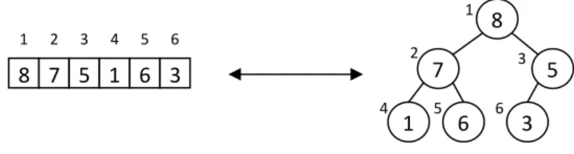
Heapsort... 37
Heaps ... 37
Sorting in a heap ... 39
Quicksort ... 40
Partition algorithm ... 40
Sorting with quicksort ... 41
Sorting in Linear Time ... 44
Lower bounds for sorting ... 44
Counting sort... 46
Radix sort ... 49
Medians and Order Statistics ... 50
Minimum and maximum ... 51
Selection in expected linear time ... 52
Selection in worst-case linear time ... 53
Dynamic Programming ... 57
Rod cutting ... 57
Recursive top-down implementation ... 60
Using dynamic programming for optimal rod cutting ... 62
Reconstructing a solution ... 65
Amortized Analysis ... 67
Two examples ... 67
Augmented stack operations ... 67
Incrementing a binary counter ... 68
Aggregate analysis ... 68
Aggregate analysis of the augmented stack operations ... 69
Aggregate analysis of incrementing a binary counter ... 69
The accounting method ... 71
Accounting method for the augmented stack operations ... 71
Accounting method for incrementing a binary counter ... 72
The potential method ... 73
Potential method for the augmented stack operations ... 74
Potential method for incrementing a binary counter... 75
Greedy Algorithms ... 77
Elements of the greedy approach ... 77
Huffman coding... 79
Graphs ... 84
Graphs and their representation ... 84
Single-source shortest path methods ... 85
Breadth-first search ... 85
Dijkstra’s algorithm ... 87
Computational Geometry ... 90
Cross products ... 90
Determining whether consecutive segments turn left or right ... 91
Determining whether two line segments intersect ... 91
Determining whether any pair of segments intersect ... 93
Ordering segments ... 94
Moving the sweep line ... 94
Correctness and running time ... 95
Finding the convex hull ... 98
Graham’s scan ... 98
References ... 100
Index ... 101
About Algorithms
In everyday life we could simply call a sequence of actions an algorithm, however, since we intend to talk about algorithms all through this course, we ought to define this notion more carefully and rigorously. A finite sequence of steps (commands, instructions) for solving a certain sort of problems is called an algorithm if it can provide the solution to the problem after executing a finite number of steps. Let us examine the properties and elements of algorithms closer.
The notion of finiteness occurs twice in the definition above. Not only does the number of steps have to be finite but each step also has to be finished in finite time (e.g., a step like “list all natural numbers” is prohibited). Another point is definiteness. Each step has to be defined rigorously, therefore the natural languages that are often ambiguous are not suitable for an algorithm’s description. We will use other methods for this purpose, like flow diagrams or pseudocodes (see later in this chapter). Moreover, an algorithm has to be executable. This means that every step of the algorithm must be executable (e.g., a division by zero is not a legal step).
Each algorithm has an input and an output. These are special sets of data in a special format. The input is a set of data that has to be given prior to beginning the execution of the algorithm but can be empty in some cases (e.g., the algorithm
“open the entrance door” has no further input, the algorithm itself determines the task). The output is a set of data, as well, however, it is never an empty set.
The output depends on the algorithm and the particular input. Both the input and the output can be of any kind of data: numbers, texts, sounds, images, etc.
Structured programming
When designing an algorithm we usually follow the top-down strategy. This method breaks up the problem to be solved by the algorithm under design into subproblems, the subproblems into further smaller parts, iterating this procedure until the resulting building blocks can be solved directly. The basic method of the top-down program design was worked out by E.W.DIJKSTRA in the 1960s (1), and says that every algorithm can be broken up into steps coming from the following three basic classes of structural elements:
• Sequence is a series of actions to be executed one after another.
• Selection is a kind of decision where only one of a given set of actions can be executed, and the algorithm determines the one.
• Iteration (also called repetition) means a frame that regulates the repeat of an action depending on a condition. The action is called the body of the iteration loop.
This means that all low or high level algorithms can be formulated as a series of structural elements consisting only of the three types above. Hence, for any algorithm description method it is enough to be able to interpret the three types above.
Algorithm description methods
There are various description methods. They can be categorized according on the age when they were born and the purpose they were invented for. From our present point of view the two most important and most widely used are flow diagrams and pseudocodes. There are several methods which support structured algorithm design better and also ones which reflect the object-oriented approach and programming techniques. But for describing structured algorithmic thoughts, methods, procedures or whatever we call them, the two mentioned above are the most convenient to use and most understandable of all.
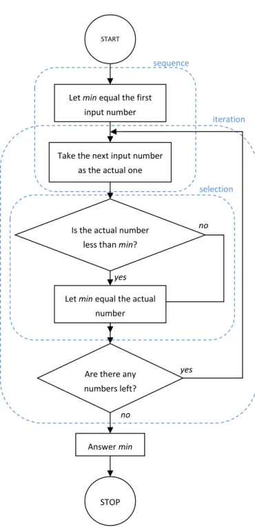
We will demonstrate the two kinds of algorithm description methods on a simple problem, the problem of finding the least number in a given set of numbers. Thus, the input is a set of numbers, usually given as a sequence, and the output the least among them. The algorithm works as follows. We consider the first number in the sequence as the actual least one, and then check the remaining numbers. If a number less than the actual minimum is found, we replace our choice with the newly found. After all numbers have been checked, the actual minimum is the minimum of all numbers at the same time.
Flow diagrams
A flow diagram consists of plane figures and arrows connecting them in a directed way. There is more than one standard, yet we have a look at only one of them here.
yes
yes
no
no
START
Let min equal the first input number
Are there any numbers left?
Take the next input number as the actual one
Is the actual number less than min?
Let min equal the actual number
Answer min
STOP
sequence
selection iteration
Figure 1. The flow diagram of the minimum finding problem.
Circle: A circle denotes a starting point or an endpoint containing one of the words START or STOP. There can be more than one endpoint but only one starting point.
Rectangle: A rectangle always contains an action (command).
Diamond: A diamond (rhombus) formulates a simple decision, it contains a yes/no question, and has two outgoing arrows denoted with a yes and a no, respectively.
The flow diagram of the problem of finding the least element can be seen in Figure 1. Examples of the three basic structural elements can be found in the light dotted frames (the frames are not part of the flow diagram).
Pseudocode
The pseudocode is the closest description method to any general structured programming language such as Algol, Pascal or C, and the structured part of Java and C#. Here we assume that the reader is familiar with the basic structure of at least one of these. The exact notation of the pseudocode dialect we are going to use is the following.
• The assignment instruction is denoted by an arrow ().
• The looping constructs (while-do, for-do, and repeat-until) and the conditional constructs (if-then and if-then-else) are similar to those in Pascal.
• Blocks of instructions are denoted by indentation of the pseudocode.
• Objects are handled as references (hence, a simple assignment between objects does not duplicate the original one, only makes a further reference to the same object). Fields of an object are separated by a dot from the object identifier (object.field). If an object reference is empty, it is referred to as a NIL value. Arrays are treated as objects but the indices are denoted using brackets, as usual.
• Parameters are passed to a procedure by value by default. For objects this means the value of the pointer, i.e., the reference.
The following pseudocode formulates the algorithm of finding the least number of a set of numbers given in an array A. Although the problem can be solved in several ways, the one below follows the structure of the flow diagram version given in Figure 1.
Minimum(A) 1 min A[1]
2 i 1 3 repeat
4 i i + 1 5 if A[i] < min 6 then min A[i]
7 until i A.Length 8 return min Exercises
1 Give a simple real-life example to the design of an algorithm using the top-down strategy. Draw a flow diagram for the algorithm.
2 Draw a flow diagram for the following task: Take a given n number of books from the shelf and put them into a bin, supposing you can hold at most h (≤ n) books at a time in your hands.
3 Write a pseudocode for the task described in the previous exercise.
4 Write a computer program simulating the task of exercise 1.
Type algorithms
Algorithms can be classified by more than one attribute, one of these is to consider the number and structure of their input and output. From this point of view four different types of algorithms can be distinguished (2).
1 Algorithms assigning a single value to a sequence of data.
2 Algorithms assigning a sequence to another sequence.
3 Algorithms assigning a sequence to more than one sequence.
4 Algorithms assigning more than one sequence to a sequence.
Some examples for the particular type algorithms are given in the following enumeration.
• Algorithms assigning a single value to a sequence are among others
o sequence calculations (e.g. summation, product of a series, linking elements together, etc.),
o decision (e.g. checking whether a sequence contains any element with a given property),
iteration selection
sequence
o selection (e.g. determining the first element in a sequence with a given property provided we know that there exists at least one), o search (e.g. finding a given element),
o counting (e.g. counting the elements having a given property), o minimum or maximum search (e.g. finding the least or the largest
element).
• Algorithms assigning a sequence to another sequence:
o selection (e.g. collect the elements with a given property of a sequence),
o copying (e.g. copy the elements of a sequence to create a second sequence),
o sorting (e.g. arrange elements into an increasing order).
• Algorithms assigning a sequence to more than one sequence:
o union (e.g. linking two sequences together excluding duplicates – set union),
o intersection (e.g. producing the set intersection of the elements of two sequences),
o difference (e.g. producing the set difference of two sequences), o uniting sorted sequences (merging / combing two ordered
sequences).
• Algorithms assigning more than one sequence to a sequence:
o filtering (e.g. filtering out elements of a sequence having given properties).
Exercises
5 Write a pseudocode that calculates the product of a series given as an array parameter.
6 Write a pseudocode that determines the index of the second least element in an unsorted array consisting of pair-wise different values. (The second least element is that which is greater than exactly one other element in the array.)
7 Write a pseudocode that finds a number that is smaller than at least one of the elements preceding it in an input array.
8 Write a pseudocode that counts how many odd numbers there are in a given array.
9 Write pseudocodes for the set operations union, intersection and difference. The sets are stored in arrays.
10 Write a pseudocode that combs two sorted arrays in a third array.
Special algorithms
As we have seen, algorithms consist of sequences of algorithmic steps (instructions) where some series of steps can be repeatedly executed (iteration).
Because of this latter feature these algorithms are jointly called iterative algorithms. An iterative algorithm usually has an initialization part consisting of steps (initialize variables, open files, etc.) to be executed prior to the iteration part itself, subsequently the loop construct is executed. However, there are algorithms slightly differing from this pattern, although they consist of simple steps in the end.
Recurrences
We call an algorithm recursive if it refers to itself. A recurrence can be direct or indirect. It is direct if it contains a reference to itself, and it is indirect if two methods are mutually calling each other.
A recursive algorithm always consists of two parts, the base case and the recursive case. The base criterion decides which of them has to be executed next. Roughly speaking, if the problem is small enough, it is solved by the base case directly. If it is too big for doing so, it is broken up into smaller subproblems that have the same structure as the original, and the algorithm is recalled for these parts. The process obviously ends when all arising subproblems “melt away”.
A typical example of a recursive solution is the problem known as the Towers of Hanoi, which is a mathematical puzzle. It consists of three rods, and a number of disks of different sizes which can slide onto any rod. The puzzle starts with the disks in a neat stack in ascending order of size on one rod, the smallest at the top, thus making a conical shape. The objective of the puzzle is to move the entire stack to another rod, obeying the following rules:
1 Only one disk may be moved at a time.
2 Each move consists of taking the upper disk from one of the rods and sliding it onto another rod, on top of the other disks that may already be on that rod.
3 No disk may be placed on top of a smaller disk.
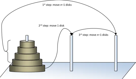
The recursive solution of moving n disks from the first rod to the second using the third one can be defined in three steps as demonstrated in Figure 2.
The pseudocode of the procedure providing every single disk move is given below.
In order to move n disks from the first to the second rod using the third one, the method has to be called with the parameters TowersOfHanoi(n,1,2,3).
TowersOfHanoi(n,FirstRod,SecondRod,ThirdRod) 1 if n > 0
2 then TowersOfHanoi(n – 1,FirstRod,ThirdRod,SecondRod) 3 write “Move a disk from ” FirstRod “ to ” SecondRod 4 TowersOfHanoi(n – 1, ThirdRod,SecondRod,FirstRod)
The base criterion is the condition formulated in line 1. The base case is n = 0 when no action is necessary. If n > 0 then all disks are moved using recurrence in lines 2 and 4.
Backtracking algorithms
Backtracking algorithms are systematic trials. They are used when during the solution of a problem a selection has to be passed without the information which is needed for the algorithm to come to a decision. In this case we choose one of the possible branches and if our choice turns out to be false, we return (backtrack) to the selection and choose the next possible branch.
1st step: move n–1 disks
2nd step: move 1 disk
3rd step: move n–1 disks
Figure 2. Three steps of recursive solution
A typical example of backtracking algorithms is the solution to the Eight Queens Puzzle where eight chess queens have to be placed on a chessboard in such a way that no two queens attack each other.
To solve the problem we place queens on the chessboard column by column selecting a row for each new queen where it can be captured by none of the ones already placed. If no such row can be found for a new queen, the algorithm steps a column back and continues with trying to replace the previously placed queen to a new safe row in its column (backtracking). The pseudocode of this procedure drawing all possible solutions is given below.
EightQueens 1 column 1
2 RowInColumn[column] 0 3 repeat
4 repeat RowInColumn[column] RowInColumn[column] + 1 5 until IsSafe(column,RowInColumn)
6 if RowInColumn[column] > 8 7 then column column – 1 8 else if column < 8
9 then column column + 1
10 RowInColumn[column] 0
11 else draw chessboard using RowInColumn 12 until column = 0
Each element of the array RowInColumn stores the row number of the queen in the column given by its index, and equals 0 if there is none. The procedure IsSafe(column,RowInColumn) returns true if a queen placed to the coordinates (column,RowInColumn[column]) is not attacked by any of the queens in the previous columns or is outside the chessboard, i.e., RowInColumn[column] > 8 here. In the latter case a backtracking step is needed in line 7.
Exercises
11 Write a pseudocode solving the warder’s problem: There is a prison having 100 cells all of which are locked up. The warder is bored, and makes up the following game. He opens all cells, then locks up every second, subsequently opens or locks up every third depending on its state, then every forth, etc. Which cells are open by the end of the warder’s “game”.
12 Write the pseudocode of IsSafe(column,RowInColumn) used in the pseudocode of EightQueens.
13 Let us suppose that there are 10 drivers at a car race. Write a pseudocode which lists all possibilities of the first three places. Modify your pseudocode so that it works for any n drivers and any first k(≤n) places. (We call this the k-permutation of n elements.)
14 Let us suppose we are playing a lottery game: we have 90 balls in a pot numbered from 1 to 90, and we draw 5 of them. Write a pseudocode which lists all possible draws. Modify your pseudocode so that it works for any n balls and any k(≤n) drawn of them. (We call this the k- combination of n elements.)
Analysis of algorithms
After an algorithm is constructed ready to solve a given problem, two main questions arise at once. The first is whether the method always gives a correct result to the problem, and the second is how it manages the resources of a computer while delivering this result. The answer to the first question is simple, it is either “yes” or “no”, even if it is usually not easy to prove the validity of this answer. Furthermore, the second question involves two fields of investigations:
that of the storage complexity and the time complexity of the algorithm.
Complexity of algorithms
Storage and time complexity are notions which express the amount of storage and time the algorithm consumes depending on the size of the input. In order to be able to interpret and compare functions describing this dependence, a piece of the used storage or time is considered as elementary if it does not depend on the size of the input. For instance, if we consider the problem of finding the minimum as seen previously, then if the cardinality of the set to be examined is denoted by n, the storage complexity turns out to be n+1, while the time complexity equals n. How do we come to these results?
The storage complexity of the algorithm is n+1 because we need n elementary storage places to store the elements to be examined, and we need one more to store the actual minimum. (For the sake of simplicity here we are disregarding the loop variable.) We do not use any unit of measurement since if an element consists of 4 bytes, then (n+1)4 bytes are needed in all, but if a single element takes 256 bytes then it is (n+1)256 bytes of storage that the algorithm occupies.
Therefore the algorithm’s tendency of storage occupation is n+1 independently of the characteristics of the input type.
Note that in reality the algorithm does not need to store all the elements at the same time. If we modified it getting the elements one by one during execution, the storage complexity would work out as 1.
The same methodology of analysis can be observed in calculating time complexity.
In our example it is n. Where does this come from? For the analysis of the algorithm we will use the pseudocode of the method Minimum (page 5) (the n=A.length notation is used here). Lines 1 and 2 are executed together and only once so they can be considered as a single elementary algorithmic step due to our definition above, i.e. the execution time of the first two lines does not depend on the input’s size. The same holds for the body of the iteration construct in lines 4 through 6, which is executed n−1 times (from i=1 to i=n−1 when entering the body). Hence the time complexity of the whole algorithm equals 1+(n−1)=n.
The asymptotic notation
If, for example two algorithmic steps can be considered as one, or even a series of tens or hundreds of steps make up a single elementary step, the question arises whether there is any sense in distinguishing between n and n+1. Since n=(n−1)+1 while n+1=(n−1)+2, and we have just learned that it is all the same whether we execute one or two steps after having taken n−1; n and n+1 seem to denote the same complexity. This is exactly the reason for using asymptotic notation which eliminates these differences and introduces a uniform notation for the complexity functions.
Let us define the following set of functions. We say that a function f has the asymptotic upper bound (or is asymptotically bounded from above by) g and we denote this as 𝑓(𝑥) = 𝑂(𝑔(𝑥)) (correctly we should use the “set element of”
notation: 𝑓(𝑥) ∈ 𝑂(𝑔(𝑥))) if
(∃𝐶, 𝑥0> 0) (∀𝑥 ≥ 𝑥0) 0 ≤ 𝑓(𝑥) ≤ 𝐶 ∙ 𝑔(𝑥)
holds. The notation is called Landau (3) notation (or big O notation). The word asymptotic is used here because the bounding property is fulfilled only from a given threshold x0 upwards, and only applying a multiplier C for the bounding function g. Using this definition all the functions 𝑓0(𝑛) = 𝑛, 𝑓1(𝑛) = 𝑛 + 1, 𝑓2(𝑛) = 𝑛 + 2, etc. are of 𝑂(𝑛) delivering the expected result, even a linear function such as 𝑓(𝑥) = 3𝑥 − 2 is 𝑂(𝑛). However, it is easy to check that all linear functions are of 𝑂(𝑛2) at the same time. This is no wonder because the O() notation formulates only an asymptotic upper bound on the function f, and n and
n2 are both upper bounds of n, although the latter one is not a tight bound. To make this bound tight, we extend our definition for the same function to be also a lower bound. We say that the function f asymptotically equals function g and we denote this relation as 𝑓(𝑥) = 𝜃(𝑔(𝑥)) if
(∃𝑐, 𝐶, 𝑥0> 0) (∀𝑥 ≥ 𝑥0) 0 ≤ 𝑐 ∙ 𝑔(𝑥) ≤ 𝑓(𝑥) ≤ 𝐶 ∙ 𝑔(𝑥)
holds. Certainly, in this case 𝑛 ≠ 𝜃(𝑛2) since no positive number c exists that satisfies the inequality 𝑐 ∙ 𝑛2≤ 𝑛 for all natural numbers.
The notion of an asymptotic lower bound can be defined in a similar way, and the notion of the proper version of asymptotic lower and upper bounds also exists but we will use only the two defined above.
Formulating time complexity
When we use asymptotic notation, the algorithm for finding the minimum of n elements has a time complexity of T(n)=O(n). A strange consequence of this notation is that due to the formal definition time complexity of finding the minimum of n numbers is the same as that of finding the minimum of 2n numbers, i.e. T(2n)=O(n). Obviously, the execution of the algorithm would take twice as long in practice. Nevertheless, the asymptotic notation delivers only the tendency of the awaited time consumption, delivering this strange result. This means that if the time complexity is O(n), i.e. linear in n, then having two, three or four times more data, the algorithm will approximately run two, three and four times longer, respectively. For instance, if an algorithm has T(n)=θ(n2) time complexity, this means that increasing the size of its input to the double or triple, it will approximately run four and nine times longer, respectively.
If we merge an algorithm’s groups of steps which are not repeated by a number of repetitions depending on the input’s size, the time complexity can easily be formulated. However, if the algorithm under consideration is recursive, this problem can be far more difficult. Let us revisit the puzzle Towers of Hanoi described on page 8. In the pseudocode the solution consists of only three steps, however, the time complexity of the recursive calls in lines 2 and 4 is not explicitly known. Moreover, we make the observation that the formula for the time complexity of any recursive algorithm is itself recursive. In this case, if we take the time complexity of the pseudocode line by line, the time complexity of the method TowersOfHanoi is the following.
𝑇(𝑛) = 1 + 𝑇(𝑛 − 1) + 1 + 𝑇(𝑛 − 1) = 2𝑇(𝑛 − 1) + 2 = 2𝑇(𝑛 − 1) + 1 The last equation looks weird from a mathematical point of view, but since this is a time complexity function, any constant number of steps can be merged into one single step.
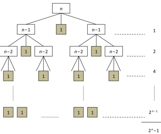
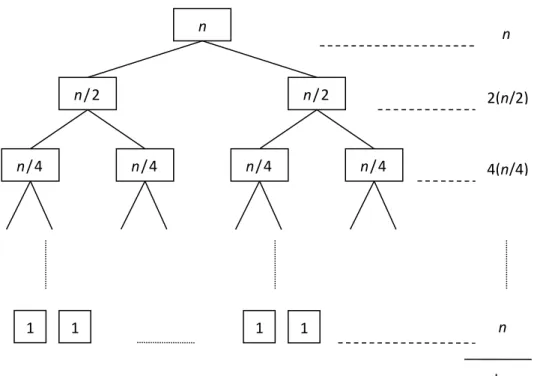
The difficulty of calculating this function is due to the recurrence in it. In this particular case it is not too hard to find the explicit formula 𝑇(𝑛) = 2𝑛− 1 but in general it is a very difficult, sometimes insoluble problem. A simple way of determining the time complexity of a recursive algorithm, or at least giving an asymptotic upper bound of it is using a recursion tree. The recursion tree of the algorithm for the problem Towers of Hanoi is shown in Figure 3.
In the recursion tree we draw the hierarchic system of the recurrences as a tree graph. Subsequently we calculate the effective number of algorithmic steps (in
n
n−1 1 n−1
n−2 1 n−2 n−2 1 n−2
1
2
1 1 1 1 4
1 1 1 1 2n−1
2n−1
Figure 3. Recursion tree of the Towers of Hanoi puzzle
this example the number of disks being moved is meant, denoted by shaded boxes in Figure 3) for each level, i.e. “row of the tree”. At the end, these sums are summarized, delivering the time complexity of the algorithm.
In our examples above the algorithms have always been supposed to work in one way only. In other words, given n elements, the way of finding the minimum does not depend on where we find it among the elements; or given n disks on one of three rods, the way of moving the disks to another rod does not depend on anything except for the initial number of disks. Nevertheless, there exist algorithms where the procedure depends also on the quality of the input, not only on the quantity of it. If the problem is to find a certain element among others (e.g., a person in a given list of names), then the operation of the algorithm can depend on where the wanted person is situated in the list. Let us consider the easiest search algorithm, the so-called linear search, taking the elements of the list one by one until it either finds the wanted one or runs out of the list.
LinearSearch(A,w) 1 i 0
2 repeat i i + 1
3 until A[i] = w or i = A.Length 4 if A[i] = w then return i 5 else return NIL
The best case is obviously if we find the element at the first position. In this case 𝑇(𝑛) = 𝑂(1). Note that to achieve this result it is enough to assume to find w in one of the first positions (i is a constant). The worst case is if it is found at either the last place or if it isn’t found at all. Thus, the number of iterations in lines 2 and 3 of the pseudocode equals the number n of elements in the list, hence 𝑇(𝑛) = 𝜃(𝑛). In general, none of the two extreme cases occur very frequently but a kind of average case operation happens. We think that this is when the element to be found is somewhere in the middle of the list, resulting in a time complexity of 𝑇(𝑛) = (𝑛 + 1) 2⁄ = 𝜃(𝑛). Indeed, the average case time complexity is defined using the mathematical notion of mean value taking all possible inputs’ time complexities into consideration. Since on a finite digital computer the set of all possible inputs is always a finite set, this way the mean value is unambiguously defined. In our example if we assume that all possible input situations including the absence of the searched element occur with the same probability this is the following.
𝑇(𝑛) =1 + 2 + 3 + ⋯ + 𝑛 + 𝑛
𝑛 + 1 =𝑛(𝑛 + 1) + 2𝑛 2(𝑛 + 1) =𝑛
2+ 𝑛 𝑛 + 1≤𝑛
2+ 1 = 𝑂(𝑛)
Exercises
15 Prove that the function 𝑓(𝑥) = 𝑥3+ 2𝑥2− 𝑥 is 𝜃(𝑥3).
16 Prove that the function 𝑓(𝑥) = 2𝑥2− 3𝑥 + 2 is 𝑂(𝑥3) but is not 𝜃(𝑥3).
17 Prove that the time complexity of the Towers of Hanoi is 𝜃(2𝑛).
18 Prove that in the asymptotic notation 𝜃(log 𝑛) the magnitude of the function is independent from the base of the logarithm.
19 Determine an upper bound on the time complexity of the algorithm called the Sieve of Eratosthenes for finding all primes not greater than a given number n.
20 Determine the time complexity of the recursive algorithm for calculating the nth Fibonacci number. Compare your result with the time complexity of the iterative method.
Data Structures
Most algorithms need to store data, and except for some very simple examples, sometimes we need to store a huge amount of data in structures which serve our purposes best. Depending on the problem our algorithm solves, we might need different operations on our data. And because there is no perfect data structure letting all kinds of operation work fast, the appropriate data structure has to be chosen for each particular problem.
Linear data structures
Arrays vs. linked lists
Arrays and linked lists are both used to store a set of data of the same type in a linear ordination. The difference between them is that the elements of an array follow each other in the memory or on a disk of the computer directly, while in a linked list every data element (key) is completed with a link that points at the next element of the list. (Sometimes a second link is added to each element pointing back to the previous list element forming a doubly linked list.) Both arrays and linked lists can manage all of the most important data operations such as searching an element, inserting an element, deleting an element, finding the minimum, finding the maximum, finding the successor and finding the predecessor (the latter two operations do not mean finding the neighbors in the linear data structure, but they concern the order of the base set where the elements come from). Time complexity of the different operations (in the worst case if different cases are possible) on the two different data structures is shown in Table 1.
Arrays are easier to handle because the elements have a so-called direct-access arrangement, which means they can be directly accessed knowing their indices in constant time, whereas an element of a linked list can only be accessed indirectly through its neighbor in the list finally resulting in a linear time complexity of access in the worst case. On the other hand, an array is inappropriate if it has to be modified often because the insertion and the deletion both have a time complexity of 𝑂(𝑛) even in the average case.
Search Insert Delete Minimum Maximum Successor Predecessor
Array 𝑂(𝑛) 𝑂(𝑛) 𝑂(𝑛) 𝑂(𝑛) 𝑂(𝑛) 𝑂(𝑛) 𝑂(𝑛)
Linked list
𝑂(𝑛) 𝑂(1) 𝑂(1) 𝑂(𝑛) 𝑂(𝑛) 𝑂(𝑛) 𝑂(𝑛)
Table 1. Time complexity of different operations on arrays and linked lists (worst case).
Representation of linked lists
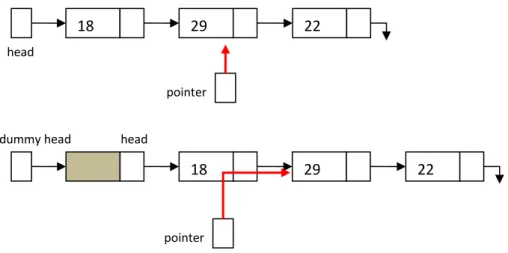
Linked lists can be implemented using record types (struct or class) with pointers as links if available in the given programming language but simple pairs of arrays will do, as well (see later in this subsection). A linked list is a series of elements each consisting of at least a key and a link. A linked list always has a head pointing at the first element of the list (upper part of Figure 4). Sometimes dummy head lists are used with single linked lists where the dummy head points at the leading element of the list containing no key information but the link to the first proper element of the list (lower part of Figure 4).
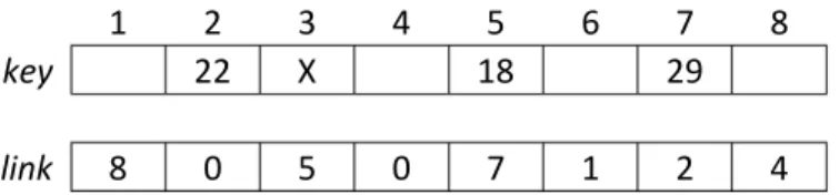
All kinds of linked lists can be implemented as arrays. In Figure 5 the dummy head linked list of Figure 4 is stored as a pair of arrays. The dummy head contains the index 3 in this example.
18 29 22
18 29 22
head
dummy head head
pointer pointer
Figure 4. The same keys stored in a simple linked list and a dummy head linked list.
The advantage of dummy head linked lists is that they promote the usage of double indirection (red arrow in the lower part of Figure 4) by making it possible to access the first proper element in a similar way like any other element. On the other hand, double indirection maintains searching a position for an insertion or a deletion. This way after finding the right position, the address of the preceding neighbor is kept stored in the search pointer. For instance, if the element containing the key 29 in Figure 4 is intended to be deleted, then the link stored with the element containing 18 has to be redirected to point at the element containing 22. However, using a simple linked list (upper part of Figure 4) the address of 18 is already lost by the time 29 is found for deletion.
The following two pseudocodes describe the algorithm of finding and deleting an element from a list on a simple linked list and a dummy head linked list, respectively, both stored in a pair of arrays named key and link.
FindAndDelete(toFind,key,link) 1 if key[link.head] = toFind 2 then toDelete link.head 3 link.head link[link.head]
4 Free(toDelete,link)
5 else toDelete link[link.head]
6 pointer link.head
7 while toDelete 0 and key[toDelete] toFind
8 do pointer toDelete
9 toDelete link[toDelete]
10 if toDelete 0
11 then link[pointer] link[toDelete]
12 Free(toDelete,link)
Figure 5. A dummy head linked list stored in a pair of arrays. The dummy head is pointing at 3.
The head of the garbage collector list is pointing at 6.
1 2 3 4 5 6 7 8
key 22 X 18 29
link 8 0 5 0 7 1 2 4
Procedure Free(index,link) frees the space occupied by the element stored at index. In lines 1-4 given in the pseudocode above the case is treated when the key to be deleted is stored in the first element of the list. In the else clause beginning in line 5 two pointers (indices) are managed, pointer and toDelete. Pointer toDelete steps forward looking for the element to be deleted, while pointer is always one step behind to enable it to link the element out of the list if once found.
The following realization using a dummy head list is about half as long as the usual one. It does not need an extra test on the first element and does not need two pointers for the search either.
FindAndDeleteDummy(toFind,key,link) 1 pointer link.dummyhead
2 while link[pointer] 0 and key[link[pointer]] toFind 3 do pointer link[pointer]
4 if link[pointer] 0
5 then toDelete link[pointer]
6 link[pointer] link[toDelete]
7 Free(toDelete,link)
Dummy head linked lists are hence more convenient to use for storing lists, regardless of whether they are implemented with memory addresses or indices of arrays.
In Figure 5 the elements seem to occupy the space randomly. Situations like this often occur if several insertions and deletions are done continually on a dynamic linked list stored as arrays. The problem arises where a new element should be stored in the arrays. If we stored a new element at position 8, positions 1, 4 and 6 would stay unused, which is a waste of storage. Nevertheless, if after this a new element came again, we would find no more free storage (position 9 does not exist here). To avoid situations like these, a kind of garbage collector can be used.
This means that the unused array elements are threaded to a linked list, simply using the index array link (in Figure 5 the head of this list is pointing at 6). Thus, if a new element is inserted into the list, its position will be the first element of the garbage list; practically the garbage list’s first element is linked out of the garbage list and into the proper list (Allocate(link)) getting the new data as its key. On the other hand, if an element is deleted, its position is threaded to the garbage list’s beginning (Free(index,link)). Initially, the list is empty and all elements are in the garbage list.
The following two pseudocodes define the algorithms for Allocate(link) and Free(index,link).
Allocate(link)
1 if link.garbage = 0 2 then return 0
3 else new link.garbage
4 link.garbage link[link.garbage]
5 return new
If the garbage collector is empty (garbage = 0), there is no more free storage place in the array. This storage overflow error is indicated by a 0 return value.
The method Free simply links in the element at the position indicated by index to the beginning of the garbage collector.
Free(index,link)
1 link[index] link.garbage 2 link.garbage index
Stacks and queues
There are some data structures from which we require very simple operations.
The simplest basic data structures are stacks and queues. Both of them have only two operations: putting an element in and taking one out, but these operations have to work very quickly, i.e. they need to have constant time complexity. (These two operations have extra names for stacks; push and pop, respectively.) The difference between stacks and queues is only that while a stack always returns the last element which was put into it (this principle is called LIFO = Last In First Out), a queue delivers the oldest one every time (FIFO = First In First Out). An example for stacks is the garbage collector of the previous subsection where the garbage stack is implemented as a linked list. Queues are used in processor “pipelines”, for instance, where instructions are waiting to be executed, and the one that has been waiting most is picked up from the queue and executed next.
Both stacks and queues can be implemented using arrays or linked lists. If a stack is represented with an array, an extra index variable is necessary to store where the last element is. If a linked list is used, the top of the stack is at the beginning of the list (no dummy head is needed). For the implementation of queues as linked lists an extra pointer is defined to point at the last element of the list. Hence new
elements can be put at the end of the list and picked up at the beginning, both in constant time. If an array stores a queue, the array has to be handled cyclically (the last element is directly followed by the first). This way it can be avoided to come to the end of the array while having plenty of unused space at the beginning of it.
For both stacks and queues two erroneous operations have to be handled:
underflow and overflow. Underflow happens if an element is intended to be extracted from an empty data structure. Overflow occurs if a new element is attempted to be placed into the data structure while there is no more free space available.
The following pseudocodes implement the push and pop operations on a stack stored in a simple array named Stack. The top of the stack index is stored in the Stack object’s field top (in reality it can be the 0th element of the array, for instance).
Push(key,Stack)
1 if Stack.top = Stack.Length 2 then return Overflow error 3 else Stack.top Stack.top + 1 4 Stack[Stack.top] key
If Stack.top is the index of the last element in the array, then the stack is full and the overflow error is indicated by the returned value. The next pseudocode indicates the underflow error in the same way. Note that in this case the value indicating the error has to differ from all possible proper output values that can normally occur (i.e. values that are stored in the stack).
Pop(Stack)
1 if Stack.top = 0
2 then return Underflow error 3 else Stack.top Stack.top − 1 4 return Stack[Stack.top + 1]
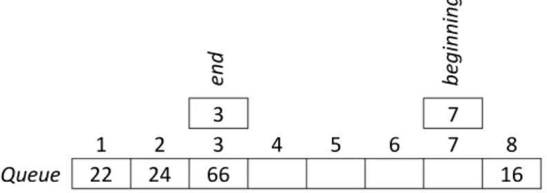
The next two pseudocodes define the two basic operations on a queue stored in a simple array. The beginning and the end of the queue in the array are represented by two indices; Queue.end is the index of the last element, and Queue.beginning is the index of the element preceding the queue’s first element in a cyclic order (see Figure 6).
The coding of the empty queue has to be planned thoughtfully. A good solution can be to let the beginning be the index of the array’s last element (Length) and end be 0. Hence a difference can be made between an empty and a full queue.
Enqueue(key,Queue)
1 if Queue.beginning = Queue.end 2 then return Overflow error
3 else if Queue.end = Queue.Length
4 then Queue.end 1
5 else Queue.end Queue.end + 1 6 Queue[Queue.end] key
Stepping cyclically in the array is realized in lines 3-5 in both of the pseudocodes Enqueue and Dequeue.
Dequeue(Queue) 1 if Queue.end = 0
2 then return Underflow error
3 else if Queue.beginning = Queue.Length 4 then Queue.beginning 1
5 else Queue.beginning Queue.beginning + 1 6 key Queue[Queue.beginning]
7 if Queue.beginning = Queue.end
8 then Queue.beginning Queue.Length
9 Queue.end 0
10 return key
In lines 7-10 the coding of the empty queue is restored if it was the last element that has just been dequeued.
Figure 6. A possible storing of the sequence 16, 22, 24 and 66 in a queue coded in an array.
end beginning
3 7
1 2 3 4 5 6 7 8
Queue 22 24 66 16
Exercises
21 Write a pseudocode that inserts a given key into a sorted linked list, keeping the order of the list. Write both versions using simple linked lists and dummy head lists stored in a pair of arrays.
22 Write a pseudocode for both the methods push and pop if the stack is stored as a linked list coded in a pair of arrays. Does it make sense to use garbage collection in this case? Does it make sense to use a dummy head linked list? Why?
Hash tables
Many applications require a dynamic set that supports only the dictionary operations insert, search, and delete. For example, a compiler that translates a programming language maintains a symbol table, in which the keys of elements are arbitrary character strings corresponding to identifiers in the language.
Direct-address tables
Direct addressing is a simple technique that works well when the universe 𝑈 of keys is reasonably small. Suppose that an application needs a dynamic set in which each element has a key drawn from the universe 𝑈, where |𝑈| is not too large.
We shall assume that no two elements have the same key.
To represent the dynamic set, we use an array, or direct-address table, denoted by 𝑇 of the same size as 𝑈, in which each position, or slot, corresponds to a key in the universe 𝑈. For example if 𝑈 = {1,2, … ,10}, and from the universe 𝑈 the keys {2,5,7,8} are stored in the direct-address table, then each key is stored in the slot with the corresponding index, i.e. the key 2 is stored in 𝑇[2], 5 in 𝑇[5], etc. The remaining slots are empty (e.g. they store a NIL value). It is similar to a company’s parking garage, where every employee has its own parking place (slot). Obviously, all three operations can be performed in 𝑂(1), namely in constant time.
Exercises
23 Suppose that a dynamic set 𝑆 is represented by a direct-address table 𝑇 of length 𝑚. Describe a procedure that finds the maximum element of 𝑆. What is the worst-case performance of your procedure?
24 A bit vector is simply an array of bits (0s and 1s). A bit vector of length 𝑚 takes much less space than an array of 𝑚 numbers. Describe how to use a bit vector to represent a dynamic set of distinct elements. Dictionary operations should run in constant time.
Hash tables
The downside of direct addressing is obvious: if the universe 𝑈 is large, storing a table 𝑇 of size |𝑈| may be impractical, or even impossible, given the memory available on a typical computer. Furthermore, the set 𝐾 of keys actually stored may be so small relative to 𝑈 that most of the space allocated for 𝑇 would be wasted. In our parking garage example, if the employees of the firm work in shifts, then there might be many employees in all, still only a part of them uses the parking garage concurrently.
With direct addressing, an element with key 𝑘 is stored in slot 𝑘. With hashing, this element is stored in slot ℎ(𝑘); that is, we use a so-called hash function ℎ to compute the slot of the key 𝑘. Here, ℎ maps the universe 𝑈 of keys into the slots of a hash table 𝑇:
ℎ: 𝑈 → {1,2, … , |𝑇|},
where the size of the hash table is typically much less than |𝑈|. We say that an element with key 𝑘 hashes to slot ℎ(𝑘); we also say that ℎ(𝑘) is the hash value of key 𝑘.
There is one hitch: two keys may hash to the same slot. We call this situation a collision. Fortunately, we have effective techniques for resolving the conflict created by collisions.
Of course, the ideal solution would be to avoid collisions altogether. We might try to achieve this goal by choosing a suitable hash function ℎ. Because |𝑈| > |𝑇|, however, there must be at least two keys that have the same hash value; avoiding collisions altogether is therefore impossible.
Collision resolution by chaining
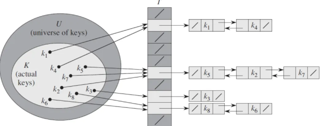
In chaining, we place all the elements that hash to the same slot into the same linked list, as Figure 7 shows. Slot j contains a pointer to the head of the list of all stored elements that hash to 𝑗; if there are no such elements, slot 𝑗 contains NIL.
How fast are the operations if chaining is used? Insertion takes obviously constant time by inserting the key 𝑘 as the new leading element of the linked list of slot ℎ(𝑘). Note, that this is only possible if it is sure that 𝑘 is not already present in the hash table. Otherwise, we have to search for 𝑘 first. The same is true for deletion.
If we know the position (i.e. the address) of key 𝑘 to be deleted, then it simply has to be linked out of its list. Otherwise, we have to find it first. The question remains how long it takes to search for an element in a hash-table. Assuming that calculating the hash function ℎ takes constant time the time complexity of finding an element in an unsorted list depends mainly on the length of the list.
The worst-case behavior of hashing with chaining is terrible: all |𝑈| keys hash to the same slot. The worst-case time for searching is thus not better than if we used one linked list for all the elements.
The average-case performance of hashing depends on how well the hash function ℎ distributes the set of keys to be stored among the slots, on the average. Therefor we shall assume that any given element is equally likely to hash into any of the slots, independently of where any other element has hashed to. We call this the assumption of simple uniform hashing. Let us define the load factor 𝛼 for 𝑇 as
|𝑈|/|𝑇|. Due to the simple uniform hashing assumption the expected value of a single chain’s length in our hash table equals 𝛼. If we add the constant time of calculating the hash function ℎ, we have the average case of operations of a hash table as 𝑂(1 + 𝛼). Thus, if we assume that |𝑈| = 𝑂(|𝑇|), i.e. 𝑈 is only linearly
Figure 7. Collision resolution by chaining. Each hash-table slot 𝑻[𝒋] contains a linked list of all the keys whose hash value is 𝒋. For example, 𝒉(𝒌𝟏) = 𝒉(𝒌𝟒) and 𝒉(𝒌𝟓) = 𝒉(𝒌𝟐) = 𝒉(𝒌𝟕). The linked list can be either singly or doubly linked; we show it as doubly linked
because deletion is faster that way.
bigger than 𝑇, then the operations in a hash table can be reduced to an average time complexity of 𝑂(1).
But how does a good hash function look like? The simplest way to create a hash function fulfilling the simple uniform hashing is using the so-called division method. We assume that the keys are coded with the natural numbers ℕ = {0,1,2, … , |𝑈| − 1}, and define the hash function as follows: for any key 𝑘 ∈ 𝑈 let ℎ(𝑘) = 𝑘 mod |𝑇|. Another solution is if the keys 𝑘 are random real numbers independently and uniformly distributed in the range 0 ≤ 𝑘 < 1, then the hash function can be defined as ℎ(𝑘) = ⌊𝑘 ∙ |𝑇|⌋. This satisfies the condition of simple uniform hashing, as well.
Exercises
25 Demonstrate what happens when we insert the keys 5, 28, 19, 15, 20, 33, 12, 17, 10 into a hash table with collisions resolved by chaining. Let the table have 9 slots, and let the hash function be ℎ(𝑘) = 𝑘 mod 9.
26 Professor Marley hypothesizes that he can obtain substantial performance gains by modifying the chaining scheme to keep each list in sorted order. How does the professor’s modification affect the running time for successful searches, unsuccessful searches, insertions, and deletions?
27 Suppose that we are storing a set of 𝑛 keys into a hash table of size 𝑚. Show that if the keys are drawn from a universe U with |𝑈| > 𝑛𝑚, then 𝑈 has a subset of size 𝑛 consisting of keys that all hash to the same slot, so that the worst-case searching time for hashing with chaining is 𝜃(𝑛).
Binary search trees
All structures above in this section are linear, preventing some basic operations from providing better time complexity results in the worst case than n (the number of stored elements). Binary search trees have another structure.
Binary search trees are rooted trees (trees are cycleless connected graphs), i.e.
one of the vertices is named as the root of the tree. A rooted tree is called binary if one of the following holds. It is either empty or consists of three disjoint sets of vertices: a root and the left and right subtrees, respectively, which are themselves binary trees. A binary tree is called a search tree if a key is stored in each of its vertices, and the binary search tree property holds, i.e. for every vertex all keys in its left subtree are less and all in its right subtree are greater than the key stored in it. Equality is allowed if equal keys can occur.
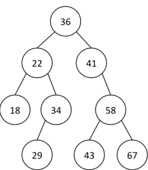
The vertices of binary trees can be classified into levels depending on their distance from the root (distance is the number of edges on the path) hence the root alone constitutes the 0th level. For instance in Figure 8 the vertex containing the number 29 is at level 3. The depth of a binary tree (sometimes also called height) is the number of the deepest level. Furthermore a vertex directly preceding another on the path starting at the root is called its parent, and the vertex following its parent directly is called child. The two children of the same vertex are called twins or siblings. A vertex without children is a leaf.
Binary search trees can be represented with dynamic data structures similar to doubly linked lists but in this case every tree element (vertex) is accompanied by three links, two for the left and the right child, respectively, and one for the parent.
Figure 8. A binary search tree.
36
41 22
18 34
29
58
43 67
Binary search tree operations
For a binary search tree, the following operations are defined: walk (i.e. listing), search, minimum (and maximum), successor (and predecessor), insert, delete.
In a linear data structure it is no question which the natural order of walking the elements is. However, a binary tree has no such obvious order. A kind of tree walk can be defined considering the binary tree as a triple consisting of the root and its two subtrees. The inorder tree walk of a binary tree is defined recursively as follows. First we walk the vertices of the left subtree using an inorder tree walk, then visit the root, and finally walk the right subtree using an inorder walk again.
There are so-called preorder and postorder tree walks, which differ from the inorder only in the order of how these three, well-separable parts are executed.
In the preorder case the root is visited first before the two subtrees are walked recursively, and in the postorder algorithm the root is visited last. It is easy to check that in a binary search tree the inorder tree walk visits the vertices in an increasing order regarding the keys. This comes from the simple observation that all keys visited prior to the root of any subtree are less than the key of that root, whilst any key visited subsequently is greater.
The pseudocode of the recursive method for the inorder walk of a binary tree is the following. It is assumed that the binary tree is stored in a dynamically allocated structure of objects where Tree is a pointer to the root element of the tree.
InorderWalk(Tree) 1 if Tree NIL
2 then InorderWalk(Tree.Left) 3 visit Tree, e.g. check it or list it 4 InorderWalk(Tree.Right)
The tree search highly exploits the special order of keys in binary search trees.
First it just checks the root of the tree for equality with the searched key. If they are not equal, the search is continued at the root of either the left or the right subtree, depending on whether the searched key is less than or greater than the key being checked. The algorithm stops if either it steps to an empty subtree or the searched key is found. The number of steps to be made in the tree and hence the time complexity of the algorithm equals the depth of the tree in worst case.
The following pseudocode searches key toFind in the binary search tree rooted at Tree.
TreeSearch(toFind,Tree)
1 while Tree NIL and Tree.key toFind 2 do if toFind < Tree.key
3 then Tree Tree.Left 4 else Tree Tree.Right 5 return Tree
Note that the pseudocode above returns with NIL if the search was unsuccessful.
The vertex containing the minimal key of a tree is the leftmost leaf of it (to check this simply let us try to find it using the tree search algorithm described above).
The algorithm for finding this vertex simply keeps on stepping left starting at the root until it arrives at an absent left child. The last visited vertex contains the minimum in the tree. The maximum is symmetrically on the other side of the binary search tree, it is the rightmost leaf of it. Both algorithms walk down in the tree starting at the root so their time complexity is not more than the depth of the tree.
TreeMinimum(Tree) 1 while Tree.Left NIL 2 do Tree Tree.Left 3 return Tree
To find the successor of a key stored in a binary search tree is a bit harder problem.
While, for example, the successor 41 of key 36 in Figure 8 is its right child, the successor 29 of 22 is only in its right subtree but not a child of it, and the successor 36 of 34 is not even in one of its subtrees. To find the right answer we have to distinguish between two basic cases: when the investigated vertex has a nonempty right subtree, and when it has none. To define the problem correctly:
we are searching the minimal key among those greater than the investigated one;
this is the successor. If a vertex has a nonempty right subtree, then the minimal among the greater keys is in its right subtree, furthermore it is the minimum of that subtree (line 2 in the pseudocode below). However, if it has none, then the searched vertex is the first one on the path leading upwards in the tree starting at the investigated vertex which is greater than the investigated one. At the same time this is the first vertex we arrive at through a left child on this path. In lines 4- 6 of the following pseudocode the algorithm keeps stepping upwards until it either finds a parent-left child relation, or runs out of the tree at the top (this could only happen if we tried to find the successor of the greatest key in the tree, which