The Long-Run Real Effects of Monetary Shocks: Lessons from a Hybrid Post-Keynesian-Dsge-Agent-Based Menu Cost Model

(1)

Journal Pre-proof

THE LONG-RUN REAL EFFECTS OF MONETARY SHOCKS: LESSONS FROM A HYBRID POST-KEYNESIAN-DSGE-AGENT-BASED MENU COST MODEL Miklós. Váry

PII: S0264-9993(21)00263-7

DOI: https://doi.org/10.1016/j.econmod.2021.105674 Reference: ECMODE 105674

To appear in: Economic Modelling Received Date: 20 July 2020 Revised Date: 31 August 2021 Accepted Date: 1 September 2021

Please cite this article as: Váry, M., THE LONG-RUN REAL EFFECTS OF MONETARY SHOCKS:

LESSONS FROM A HYBRID POST-KEYNESIAN-DSGE-AGENT-BASED MENU COST MODEL Economic Modelling, https://doi.org/10.1016/j.econmod.2021.105674.

This is a PDF file of an article that has undergone enhancements after acceptance, such as the addition of a cover page and metadata, and formatting for readability, but it is not yet the definitive version of record. This version will undergo additional copyediting, typesetting and review before it is published in its final form, but we are providing this version to give early visibility of the article. Please note that, during the production process, errors may be discovered which could affect the content, and all legal disclaimers that apply to the journal pertain.

(2)

THE LONG-RUN REAL EFFECTS OF MONETARY SHOCKS:

LESSONS FROM A HYBRID POST-KEYNESIAN-DSGE-AGENT-BASED MENU COST MODEL

Miklós Váry

Author information Given name: Miklós Family name: Váry

Affiliation 1: University of Pécs – Faculty of Business and Economics – Centre of Excel- lence of Economic Studies

Affiliation address 1: Rákóczi út 80., H-7622 Pécs, Hungary

Affiliation 2: Corvinus University of Budapest – Institute of Economics Affiliation address 2: Fővám tér 8., H-1093 Budapest, Hungary

Affiliation 3: Centre for Economic and Regional Studies – Institute of Economics Affiliation address 3: Tóth Kálmán utca 4., H-1097 Budapest, Hungary

E-mail address: miklos.vary@uni-corvinus.hu

Corresponding author: Miklós Váry, Corvinus University of Budapest – Institute of Eco- nomics, Fővám tér 8., H-1093 Budapest, Hungary (e-mail: miklos.vary@uni-corvinus.hu) Acknowledgments: I would like to thank Tamás Mellár, Ádám Reiff, Péter Bauer, Tamás Sebestyén, István Kónya, István Bessenyei, János Barancsuk, Kristóf Németh, Erik Braun, two anonymous referees, and the editor for their helpful and insightful comments. All remaining errors are mine.

Funding sources: This work was supported by the Thematic Excellence Program 2020 – Institutional Excellence Sub-program of the Ministry for Innovation and Technology in Hungary, within the framework of the University of Pécs’s 4th thematic program “En- hancing the Role of Domestic Companies in the Reindustrialization of Hungary” [grant number: 2020-4.1.1.-TKP2020] and the Pallas Athéné Domus Educationis Foundation of the Central Bank of Hungary.

The funding sources had no involvement in the study design, collection, analysis, and interpretation of the data, report writing, and the decision to submit the article for pub- lication.

Declarations of interest: none.

Journal Pre-proof

(3)

THE LONG-RUN REAL EFFECTS OF MONETARY SHOCKS:

LESSONS FROM A HYBRID POST-KEYNESIAN-DSGE-AGENT-BASED MENU COST MODEL

Abstract

This paper studies the long-run effects of monetary policy on real economic activity. It presents a hybrid menu cost model, the structure of which mimics that of dynamic stochastic general equilibrium models with fixed price adjustment costs (menu costs). It contains two mechanisms capable of generating long-run real effects in response to monetary shocks according to post- Keynesian macroeconomists, and its behavior is studied via agent-based simulations. After being calibrated to reproduce key features of the microdata, the model estimates that a typical monetary shock has substantial long-run real effects, with around one-quarter of the shock being absorbed by real output. However, the long-run effectiveness of a monetary shock turns out to decrease with its size. The key mechanisms generating long-run real effects are shown to be demand–supply interactions, that is, positive feedbacks from aggregate demand to aggregate supply. The results suggest that central banks should stronger emphasize stabilizing real economic activity when designing their monetary policies.

Journal of Economic Literature (JEL) codes: E12, E31, E32, E37, E52

Keywords: long-run monetary non-neutrality, monetary shocks, menu costs, demand–

supply interactions, post-Keynesian monetary macroeconomics, agent-based modeling

Journal Pre-proof

(4)

1

1. INTRODUCTION

Long-run monetary neutrality (LRMN) is a cornerstone of mainstream monetary macroeconomics. Money is said to be neutral in the long run if a permanent unanticipated shock to the level of the money supply does not permanently affect real economic activity (Lucas, 1996; Bullard, 1999).¹ Robert Lucas summarized the conventional wis- dom about LRMN in his Nobel Lecture as follows: “… [long-run] monetary neutrality… … needs to be a central feature of any monetary or macroeconomic theory that claims empir- ical seriousness” (Lucas, 1996, p. 666).

The long-run neutrality of money has important implications for the practice of monetary policy. If it holds, all the effects that central banks may exert on real economic activity are realized in the short run. In the long run, the price level will absorb all changes induced by the central bank in nominal aggregate demand. Although monetary policy may be effective in the short run because of price and wage rigidity, central banks should focus on maintaining low and stable inflation rates and smoothing short-run cy- clical fluctuations, as they cannot influence real economic activity in the long run. Thus, LRMN is a core pre-assumption behind the optimality of the policy of strict inflation targeting suggested to central banks by early New Keynesian monetary theories (Wood- ford, 2003; Galí, 2008).

Despite its widespread acceptance, the empirical evidence regarding LRMN is far from unambiguous.² Several empirical studies, based on post-war data from the United States (U.S.), confirm that LRMN holds (Boschen and Otrok, 1994; Boschen and Mills, 1995; King and Watson, 1997). However, it is rejected to hold if the sample contains the Great Depression (Fisher and Seater, 1993). The decision to accept or reject the LRMN hypothesis is sensitive to the country considered (Olekalns, 1996; Haug and Lucas, 1997), the monetary aggregate used to measure the money supply (Weber, 1994; Coe and Nason, 1999), and the number and location of structural breaks allowed in the long- run trends of real output, and the money supply (Noriega et al., 2008; Ventosa- Santaulària and Noriega, 2015). Atesoglu (2001) and Atesoglu and Emerson (2009) found evidence against LRMN even in post-war samples from the U.S. De Grauwe and Costa Storti (2004) argued that the reason why monetary policy has no long-run real effects according to many structural vector autoregression (SVAR) studies is that LRMN is often used as an assumption to identify exogenous monetary policy shocks. When ap- plying different identifying assumptions, monetary policy usually turns out to have long- run real effects. In a recent empirical study, Jorda et al. (2020) identified exogenous monetary policy shocks using instrumental variable methods and applied a local projec- tion method to estimate the long-run effects of these shocks on real output, which turned out to be significant.

1 This paper does not deal with the issue of long-run monetary superneutrality, that is, the question of whether permanent unanticipated shocks to the growth rate of money supply affect the level of real eco- nomic activity in the long run. See Orphanides and Solow (1990) for a comprehensive survey about the theoretical literature of long-run monetary superneutrality.

2 See Bullard (1999) for an excellent survey about the empirical literature of long-run monetary neutrality and superneutrality.

Journal Pre-proof

(5)

2

If the empirical evidence against LRMN is taken seriously, the need arises to es- tablish the magnitude of the real effects that monetary policy may exert on real economic activity in the long run and identify the key channels through which these effects may be realized. This paper takes steps to fill these gaps by proposing an estimate for the magnitude of the macro-level real effects that may emerge in the long run due to heterogeneous micro-level price adjustment to monetary shocks coupled with two economic mechanisms believed to generate long-run monetary non-neutrality (LRMNN) by post- Keynesian economists. These two mechanisms are nonlinear price adjustment and demand–supply interactions. The former term is used to refer to a micro-level pricing behavior that does not react to small demand and supply shocks, while the latter is modeled as a macro-level positive feedback from aggregate demand to aggregate supply (Pa- lacio-Vera, 2005; Fontana, 2007; Fontana and Palacio-Vera, 2007; Kriesler and Lavoie, 2007). The paper clarifies the roles played by these mechanisms in the emergence of LRMNN. It studies the long-run real effects of monetary shocks with a hybrid post- Keynesian-DSGE-agent-based menu cost model. This model combines insights from dynamic stochastic general equilibrium (DSGE) models containing fixed price adjustment costs (menu costs) with ideas from post-Keynesian monetary macroeconomics, and its behavior is analyzed via agent-based simulations.

The model tries to “bridge the gap” between post-Keynesian, DSGE, and agent- based models, following the spirit of Dilaver et al. (2018), Gobbi and Grazzini (2019), and Haldane and Turrell (2019) who argue that there is a need for more hybrid models containing some agent-based features, while being directly comparable to the DSGE benchmark. The model presented in this paper fits into this hybrid modeling approach and extends it toward post-Keynesian macro models. Its structure mimics that of DSGE- type menu cost models developed for studying the short-run real effects of monetary shocks (Golosov and Lucas, 2007; Gertler and Leahy, 2008; Nakamura and Steinsson, 2010; Midrigan, 2011; Alvarez et al., 2016; Karádi and Reiff, 2019). It contains some post-Keynesian and agent-based features to make it suitable for analyzing the connections between heterogeneous micro-level price dynamics and the macro-level long-run real effects of monetary shocks. By turning the post-Keynesian and the agent-based features of the model on and off, their implications can be made clear regarding the long- run real effects of monetary shocks. Such a modeling approach facilitates comparison between post-Keynesian, DSGE, and agent-based models, while helping to clarify the economic mechanisms behind their different conclusions.

The model is calibrated to match the most important moments of two empirical distributions related to micro-level price adjustment, derived from one of the most popular empirical samples used for calibrating menu cost models, the Dominick’s dataset (Midrigan, 2011; Alvarez et al., 2016). It estimates that a typical monetary shock has substantial long-run real effects, with around one-quarter of the shock absorbed by real aggregate output in the long run. The key post-Keynesian mechanism responsible for generating LRMNN is shown to be demand–supply interactions present in the economy.

The other post-Keynesian mechanism, nonlinear price adjustment cannot explain LRMNN in an empirically relevant way within the context of the model. Still, it plays an important role in determining the magnitude of the long-run real effects of monetary shocks once they are brought to life by demand–supply interactions. The substantial long-run real effects do not imply that central banks can stimulate real economic activity

Journal Pre-proof

(6)

3

in the long run without any limitations; the long-run effectiveness of a monetary shock is shown to decrease with its size, implying nonlinearly increasing inflationary effects in the long run as a function of the shock size. The long-run real effects of monetary shocks are asymmetric in the model as prices are assumed to react differently to positive and negative shocks, in line with the empirical evidence. There is an intermediate range of the shock size, within which negative monetary shocks are more effective in the long run, but positive shocks are more effective outside of this range.

The results have important implications for the conduct of monetary policy. If the long-run real effects of monetary shocks are substantial, there is no divine coincidence (Blanchard and Galí, 2007); central banks do not simultaneously stabilize real economic activity by stabilizing the inflation rate. Short-run disinflations cause long-run damages to the real economy that their benefits might not compensate. Under such circumstanc- es, strict inflation targeting cannot be the optimal monetary policy. In addition to following their primary target of maintaining price stability, central banks should emphasize stabilizing the real economy even stronger than in the presence of a simple short-run policy trade-off. Two post-Keynesian authors, Fontana and Palacio-Vera (2007), suggest that central banks should follow a flexible opportunistic inflation targeting approach if LRMN does not hold and should not react to small inflationary shocks. Thus, they can avoid causing long-run damage to the real economy. Instead, they should wait for another exogenous shock to take inflation back to the vicinity of its target rate. Of course, a monetary restriction is unavoidable if the inflationary shock is large. However, they should react to deflationary shocks with monetary expansions, even if the shocks are small as they might lead to long-run real benefits. The results of this paper serve as ar- guments in favor of the policy of price-level targeting (Svensson, 1999; Gaspar et al., 2010) or its state-contingent variant (Evans, 2012; Bernanke, 2019). This policy re- quires the central bank to target the average rate of inflation instead of the actual one, thus compensating periods of below-average inflation with subsequent periods of above-average inflation. According to this paper’s results, this policy of maintaining loose monetary conditions until the price level returns to its targeted path after a demand-side recession, such as the global financial crisis of 2008, may successfully restore the long-run damage caused by a demand shock in the real economy.

Recently, a few New Keynesian DSGE models have been developed to study the long-run real effects of monetary shocks generated by demand–supply interactions (Galí, 2020; Jorda et al., 2020; Garga and Singh, 2021). The usual policy implication of these models is that central banks should target additional real variables besides the usually targeted inflation rate and output gap to approximate the optimal monetary policy under LRMNN. Depending on the exact nature of demand–supply interactions that lead to the failure of LRMN, the employment or unemployment rate (Galí, 2020) or the cumulative deviation of the growth rate of total factor productivity (TFP) from its steady-state value (Garga and Singh, 2021) may serve as appropriate additional targets.

Compared to these New Keynesian models, this paper comes up with four novel contri- butions as follows:

1. In the cited models, nominal rigidities are modeled according to the Calvo (1983) model of sticky price adjustment, which is well-known to be at odds with many empirical observations regarding micro-level price adjustment (Klenow and Kryvtsov, 2008; Nakamura and Steinsson, 2008). To the best of the author’s

Journal Pre-proof

(7)

4

knowledge, the model presented in this paper is the first among those developed for studying LRMNN, which is based on insights borrowed from the literature of menu cost models. The menu cost assumption makes it possible to model price adjustment based on more sophisticated microfoundations than the Calvo (1983) model. It allows the model to reproduce all important empirical observations regarding micro-level price adjustment, resulting in better-founded estimates for the real effects of monetary shocks.

2. The menu cost assumption makes it possible to model price adjustment’s nonlinear and asymmetric nature (Karádi and Reiff, 2019), which is inherited by the long-run real effects of monetary shocks. Specifically, it allows the analysis of how the size and the sign of a monetary shock influence its long-run effectiveness.

3. It investigates the role of nonlinear price adjustment besides demand–supply interactions in determining the long-run real effects of monetary shocks.

4. The applied methodology of agent-based simulations and the agent-based features of the model can also be considered novelties. They contribute to the stronger microfoundations of the model and address some concerns raised by heterodox scholars of economics regarding DSGE models.

The rest of the paper is organized as follows. Section 2 summarizes related literature. Section 3 presents the dataset used to derive the empirical distributions related to micro-level price adjustment and the key properties of the distributions, which the model should reproduce. The hybrid menu cost model and its calibration are presented in Section 4. In Section 5, the model is used to estimate the long-run real effect of a standard monetary shock. The key mechanisms responsible for determining the long- run real effect are studied in Section 6. Section 7 analyzes how its size and its sign influence the long-run effectiveness of a monetary shock. Section 8 concludes the paper.

2. RELATED LITERATURE

The research is related to four different fields of the economic literature: post- Keynesian monetary macroeconomics, DSGE-type menu cost models, agent-based economic modeling, and New Keynesian models of long-run monetary non-neutrality.

Post-Keynesian monetary macroeconomics: To study the long-run real effects of monetary shocks, one must find economic mechanisms that can potentially explain them. Such mechanisms can most easily be found in the post-Keynesian literature, as post-Keynesians have never believed that money is neutral in the long run (Davidson, 1987, 1988; Cottrell, 1994). The literature mentions two economic mechanisms that may explain the violation of LRMN: nonlinear price adjustment and the presence of demand–supply interactions in the economy (Palacio-Vera, 2005; Fontana, 2007; Fontana and Palacio-Vera, 2007; Kriesler and Lavoie, 2007).

Nonlinear price adjustment: Within an intermediate range of the output gap, pric- es do not adjust to exogenous shocks; therefore, the short- and long-run Phillips curves are horizontal (Palacio-Vera, 2005; Kriesler and Lavoie, 2007). The following are the two most popular post-Keynesian explanations for this nonlinearity in price adjustment.

First, in a fundamentally uncertain economic environment (Keynes, 1921; Knight, 1921),

Journal Pre-proof

(8)

5

firms perceive a range of capacity utilization rates as normal, none of which induces any demand-led pressure to change prices. Second, decreasing returns do not prevail in the vicinity of potential output; hence, demand shocks lead to price adjustment only if they are large enough for decreasing returns to appear in production.

Demand–supply interactions: Potential real economic activity is path-dependent;

fluctuations in the output gap (determined by aggregate demand) affect the potential output (aggregate supply)³ (Palacio-Vera, 2005; Fontana, 2007; Fontana and Palacio- Vera, 2007; Kriesler and Lavoie, 2007). This positive feedback from actual toward potential real activity can manifest itself through three possible channels:⁴

1. Labor force: Large negative demand shocks may increase long-term unemploy- ment. The loss of skills for the long-term unemployed reduces their employabil- ity, decreasing the potential labor force (Phelps, 1972; Cross, 1987). An insider- outsider mechanism of wage bargaining, during which the employed bargain for the highest expected real wage that allows them to stay employed, may also hin- der reemployment (Blanchard and Summers, 1986, 1987; Galí, 2015, 2020).

2. Capital stock: If firms must face sunk adjustment costs related to market entry (Baldwin and Krugman, 1989; Dixit, 1989, 1992) or the initiation of their invest- ment activities (Bassi and Lang, 2016), then as the demand shock dies away, the capital stock may not return to its initial value, leading to lower potential output.

The interdependence between profits and investments may also lead to a permanently smaller capital stock when firms’ profitability is low, such as during recessions (Arestis and Sawyer, 2009). This may also slow down technological progress as innovations are often manifested in the form of capital goods (Solow, 1960).

3. Technological progress: If technological progress is endogenous, it may also slow as a result of a positive feedback from short-run economic growth to the growth rate of productivity, known as the Kaldor-Verdoorn law (Verdoorn, 1949; Kaldor, 1957; Setterfield, 2002; Dutt, 2006; Storm and Naastepad, 2012). It captures the weakening of learning by doing and firms’ reduced profit incentives to engage in research and development during recessions.

These effects work in the opposite direction for positive demand shocks.^{5, 6}

3 This positive feedback is often labeled as demand-led growth or hysteresis in the post-Keynesian litera- ture (Fontana, 2007; Fontana and Palacio-Vera, 2007; Kriesler and Lavoie, 2007). Following Arestis and Sawyer (2009), I prefer using the term demand–supply interactions, as hysteresis refers to a general prop- erty of a dynamic system, meaning that transitory shocks have permanent effects on its steady state (Am- able et al., 1993; Cross, 1993; Göcke, 2002). The possible mechanisms behind hysteresis include demand–

supply interactions, but other mechanisms may also result in hysteretic macrodynamics (Setterfield, 2009).

4 See Arestis and Sawyer (2009) for an exhaustive discussion about the role of demand–supply interactions in generating path-dependent macrodynamics.

5 However, the empirical evidence for the effects of positive demand shocks on potential real economic activity is weaker than that for the effects of negative ones (Ball, 2009).

6 There is little empirical evidence about the relative importance of the three mentioned channels in generating LRMNN, but the estimates of Jorda et al. (2020) suggest that demand–supply interactions through

Journal Pre-proof

(9)

6

DSGE-type menu cost models: The first post-Keynesian explanation for the failure of LRMN, nonlinear price adjustment is present in numerous New Keynesian macro models as well but with a different interpretation according to which firms have to face fixed adjustment costs when they change their prices (Barro, 1972; Sheshinski and Weiss, 1977; Akerlof and Yellen, 1985; Blanchard and Kiyotaki, 1987). These fixed costs of price adjustment are usually labeled as menu costs (Mankiw, 1985). They lead to the appearance of an inaction band around the flexible-price level of output, within which firms will not adjust their prices in response to demand shocks, as the menu cost will probably not be compensated by the benefits of price adjustment. The rest of the paper will mostly refer to the menu cost interpretation of nonlinear price adjustment for two reasons. First, it has become more popular thanks to the success of menu cost models.

Second, the model presented in Section 4 builds on many insights borrowed from the menu cost literature.

The existence of menu costs is not the only New Keynesian explanation for the rigidity of prices. Other explanations include predetermined prices (Phelps and Taylor, 1977) or wages (Fischer, 1977; Taylor, 1979), information frictions (Mankiw and Reis, 2002), frictions of consumer search (Cabral and Fishman, 2012), and the fairness con- siderations of consumers (Rotemberg, 2005). All of these have proven useful in explain- ing some empirical features of micro- or macro-level price adjustment. However, Klenow and Kryvtsov (2008) argued that state-dependent menu cost models can be more successful in reproducing the most important empirical regularities of micro-level price adjustment than time-dependent models, in which the occurrence of a price change depends only on the time spent since the last price change and not on the states of individual firms. Levy et al. (1997) and Dutta et al. (1999) measured the magnitude of menu costs in large U.S. retail chains directly and found that although the costs of print- ing price tags are small, there are substantial labor costs related to price adjustment. In the case of a large industrial firm, Zbaracki et al. (2004) measured the managerial costs of making pricing decisions, the costs of informing customers, and negotiating new prices and found them to be even larger than the physical costs of price adjustment. These types of costs can be expected to remain important even in the era of digitalization, when the physical costs of price adjustment will probably decrease. Slade (1998), Aguir- regabiria (1999), and Stella (2014) inferred the magnitude of menu costs from the price observations of goods sold in grocery stores using structural econometric estimations and found it to be non-negligible. Akerlof and Yellen (1985), Mankiw (1985), and Dixit (1991) argued that even small menu costs can result in large business cycles. Consider- ing their results, the practical relevance of the menu cost assumption seems to be well- grounded, even if it is compared to alternative explanations of imperfect price adjustment.

Nowadays, the menu cost assumption usually appears in DSGE models, and DSGE-type menu cost models have become the standard tools for analyzing the short- run real effects of monetary shocks (Golosov and Lucas, 2007; Gertler and Leahy, 2008;

Nakamura and Steinsson, 2010; Midrigan, 2011; Alvarez et al., 2016; Karádi and Reiff, capital accumulation may be the most important one. According to their estimates, it is followed by the TFP channel, while the labor force channel plays practically no role in generating LRMNN.

Journal Pre-proof

(10)

7

2019). However, within their framework, money is neutral in the long run despite the nonlinearity of price adjustment caused by the assumption of menu costs. This contra- dicts the views of some post-Keynesian macroeconomists (Palacio-Vera, 2005; Kriesler and Lavoie, 2007).

All of the cited DSGE-type menu cost models are heterogeneous-agent DSGE models with similar structures. The demand side of these models comprises an optimizing representative household, whose nominal income is assumed to be proportional to the nominal money supply; the central bank exogenously determines the latter. The supply side of the models consists of a continuum of ex-ante homogenous but ex-post heterogeneous firms. This means that firms follow the same dynamically optimal pricing decision rule. However, they still make different individual decisions because they are hit by idiosyncratic productivity shocks, the realizations of which differ ex-post. The assumed shape of the idiosyncratic shock distribution as well as the assumption of multiproduct firms are crucial for reproducing the shape of the empirical distribution of nonzero price changes, which, in turn, substantially influences the real effects of monetary shocks in menu cost models (Midrigan, 2011; Alvarez et al., 2016).

Agent-based economic modeling: Agent-based models are becoming increasingly popular tools in macroeconomic⁷ research (Leijonhufvud, 2006; Fagiolo and Roventini, 2017; Dawid and Delli Gatti, 2018; Dosi and Roventini, 2019; Haldane and Turrell, 2019), and specifically in monetary macroeconomics (Delli Gatti et al., 2005; Salle et al., 2013; Dosi et al., 2015; Salle, 2015). An agent-based model is “a model, in which a multi- tude of (heterogeneous) elements interact with each other and the environment” (Dawid and Delli Gatti, 2018, p. 67). Agent-based computational economics (ACE) is the applica- tion of agent-based modeling to economics or “the computational study of economic pro- cesses modeled as dynamic systems of interacting agents” (Tesfatsion, 2006, p. 835).

Standard assumptions of an ACE macro model include a large number of boundedly rational, heterogeneous agents instead of a perfectly rational, representative one and a disequilibrium market mechanism with direct local interactions of agents (Dosi, 2012;

Fagiolo and Roventini, 2017). Setterfield and Gouri Suresh (2016) argued that agent- based models are especially useful for studying path-dependent macrodynamics generated for instance by demand–supply interactions as many path-dependent phenomena are emergent. They cannot be observed at the micro-level of the economy, but they

“emerge” at the macro level as the result of interactions between heterogeneous microe- conomic agents. Agent-based models have been developed for the analysis of such emergent phenomena (Tesfatsion, 2006).⁸

Few agent-based models try to assess the differences between DSGE and ACE models by building on insights from both modeling traditions (Salle et al., 2013; Salle,

7 The most popular medium-scale agent-based macroeconomic models include the Complex Adaptive Trivial Systems (CATS) model (Delli Gatti et al., 2011; Assenza et al., 2015), the EURACE model (Deissen- berg et al., 2008; Dawid et al., 2019), the Keynes+Schumpeter (K+S) model (Dosi et al., 2010; Dosi et al., 2017), and the Java Agent-Based MacroEconomic Laboratory (JAMEL) (Seppecher, 2012; Seppecher and Salle, 2015). Some important small-scale agent-based macro models can be found, for instance, in Leng- nick (2013), Gaffeo et al. (2015), and Guerini et al. (2018).

8 Examples of agent-based models developed for studying a specific form of path-dependency, hysteresis are presented by Bassi and Lang (2016) and Dosi et al. (2018).

Journal Pre-proof

(11)

8

2015; Dilaver et al., 2018; Guerini et al., 2018; Gobbi and Grazzini, 2019). The model presented in this paper is related to these, but it cannot purely be labeled as an agent- based model because of its hybrid nature. From a methodological perspective, the model developed in this paper most closely relates to the one presented by Babutsidze (2012), which is an otherwise standard menu cost model also studied via agent-based simulations. Delli Gatti et al. (2005) presented an example of an agent-based macro model in which LRMN fails because the central bank is assumed to influence the economy through its supply side by determining the credit costs of financing production.

New Keynesian models of long-run monetary non-neutrality: In New Keynesian models of LRMNN, the long-run real effects of monetary shocks are the results of one of the following two types of demand–supply interactions: an insider-outsider mechanism of wage bargaining (Galí, 2020) or endogenous technological progress (Jorda et al., 2020; Garga and Singh, 2021). Their magnitude turns out to be economically significant under realistic calibrations.

3. THE EMPIRICAL DATA

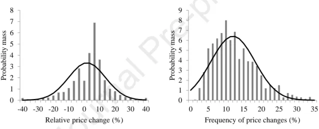
Before presenting the hybrid menu cost model, it is important to summarize the empirical observations that the model is required to reproduce. Its empirical performance will be assessed by analyzing how well it fits key moments of two empirical distributions related to product-level price adjustment: the distribution of nonzero price changes and the frequency distribution of price changes.

These two empirical distributions are derived from a micro-level dataset often applied for calibrating menu cost models, the Dominick’s dataset (Midrigan, 2011; Alva- rez et al., 2016). It consists of scanner price data collected by the James M. Kilts Center for Marketing of the University of Chicago, Booth School of Business. The dataset contains nine years (1989–1997) of weekly store-level data regarding the prices of 9,450 products collected in 86 Dominick’s Finer Foods retail chain stores in the Chicago area.

As prices are highly correlated across stores, Midrigan (2011) decided to work with prices from one store with the largest number of observations. He has made the resulting dataset available in the supplemental material to his paper, which is the dataset used in this paper. The data were collected during a period of no substantial economic tur- moil in the U.S. Thus, the calibrated model will estimate the long-run real effects of monetary shocks during normal times.

The model presented in Section 4 does not contain any incentives for firms to engage in temporary sales; therefore, the data are sales-filtered using the algorithm developed by Kehoe and Midrigan (2008) to obtain time series about regular prices.⁹ The resulting weekly time series of regular prices is time-aggregated to monthly frequency by only keeping every fourth observation. The monthly frequency of the resulting sample is closer to the quarterly frequency of GDP data that will be used to estimate some model parameters. This leaves a sample of 100 months of regular prices for 9,450 different

9 The Matlab codes for the sales-filtering algorithm and for calculating the moments of the empirical distribution of nonzero price changes are available in the Supplemental Material to Midrigan (2011). Appen- dix 1 of the same supplemental material describes the sales-filtering algorithm in detail.

Journal Pre-proof

(12)

9

products. As per Midrigan (2011), only price observations for which the calculated regular price equals the observed price are kept. Finally, all regular price changes are com- puted as the log difference of subsequent monthly prices. Following Midrigan (2011), all regular price changes with a size greater than the 99^th percentile of their size distribution are dropped to eliminate outliers. The final sample consists of 22,630 observations of nonzero monthly regular price changes.

The first step to derive the frequency distribution of empirical price changes is to calculate the frequency of monthly regular price changes for each of the 9,450 products.

This is achieved by dividing the number of months in which the product’s price has changed by the number of months for which the price observation and the previous month’s observation are not missing. Then, all products with a calculated frequency of 0 are dropped, as it seems unlikely that the price of a product does not change for nine years. Missing values are the most probable reason for not registering any price changes for these products. Finally, all products with a frequency of price changes greater than the 99^th percentile of the frequency distribution are dropped to eliminate outliers.¹⁰ The final sample consists of the frequencies of regular price changes for 7,765 products.

Note: Both histograms are based on the data available in the supplemental material to Midrigan (2011), which have been sales-filtered, time-aggregated to monthly frequency, and cleared of outliers. Superim- posed are the probability density functions of the normal distribution with equal means and variances.

Figure 1: The Empirical Distributions of Nonzero Price Changes (left panel) and of the Monthly Frequencies of Price Changes (right panel)

Figure 1 presents the two empirical distributions. The probability density func- tions of the normal distribution with equal means and variances are superimposed; they serve as benchmarks that help make the empirical distributions’ properties visible.

Graphical inspection of Figure 1, supplemented with calculating key moments of the two distributions, reveals some important empirical features of micro-level price adjustment that the model should reproduce. While calculating the moments, all price changes and

10 As the number of observations available to calculate the frequencies of price changes is different for each product, all frequencies of price changes are weighted with the number of observations available to calculate them while computing the percentiles of the frequency distribution.

0 1 2 3 4 5 6 7 8

-40 -30 -20 -10 0 10 20 30 40

Probability mass

Relative price change (%)

0 1 2 3 4 5 6 7 8 9

0 5 10 15 20 25 30 35

Probability mass

Frequency of price changes (%)

Journal Pre-proof

(13)

10

all frequencies of price changes related to a certain product are weighted with the share of that product in the basket of the average Dominick’s customer.¹¹

The empirical observations (EO) that the model will be required to reproduce are listed below,¹² reported together with the values of the moments related to the observations. All of these moments will be targeted during the calibration of the hybrid menu cost model.

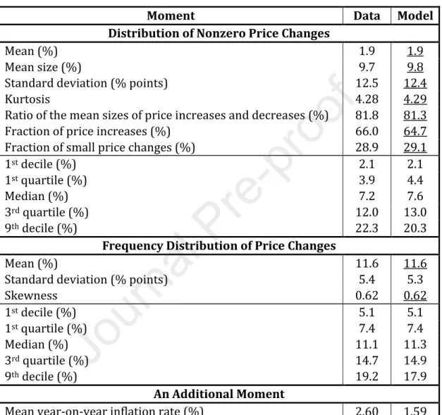
 EO1: The mean size of price changes is large (9.7%). The model needs to repro- duce this observation for the strength of price adjustment to be realistic within its framework.

 EO2: Still, many price changes are small. Specifically, 28.9% of all price changes are smaller than half of the mean size of price changes. This moment will be useful in fine-tuning the correlation between productivity shocks hitting different goods supplied by the same firm in the model.

 EO3: The simultaneous presence of many small price changes and some very large price changes implies that the distribution of nonzero price changes exhibits substantial excess kurtosis compared to the normal distribution (4.28 versus 3.00). Alvarez et al. (2016) proved that it is crucial for all menu cost models to reproduce the empirical kurtosis of nonzero price changes as it sufficiently summarizes information about the strength of the so-called selection effect, that is, the effect that price adjuster firms are not randomly selected, as in the Calvo (1983) model of sticky price adjustment, but firms with larger differences between the actual and desired prices of their products are more likely to respond to an exogenous shock with a price change. The strength of the selection effect plays an important role in determining the short-run real effects of monetary shocks in menu cost models (Caplin and Spulber, 1987; Golosov and Lucas, 2007; Midrigan, 2011). It seems reasonable to suspect that it also strongly influences the long-run real effects once they are brought to life by an appropriate mechanism.

 EO4: The standard deviation of price changes is large (12.5%). This moment will be used to pin down the standard deviation of idiosyncratic productivity shocks in the model.

 EO5: The mean nonzero price change is 1.9%. This moment will be useful for gen- erating a realistic rate of trend inflation in the model.

 EO6: Price increases are more frequent than price decreases. Specifically, 66.0% of all price changes are price increases.

 EO7: The mean size of price decreases (11.0%) is larger than that of price increases (9.0%); the latter is 81.8% of the former. EO6 and EO7 are important to repro-

11 The frequencies of price changes are also weighted with the number of observations available to calculate them, as it is different for each product because of the missing values present in the dataset.

12 These empirical observations can be considered as standard: they have all been reported before in the empirical literature of sticky price adjustment (Bils and Klenow, 2004; Klenow and Kryvtsov, 2008;

Nakamura and Steinsson, 2008). Müller and Ray (2007) and Chen et al. (2008) present detailed empirical evidence for the two observations concerning asymmetric price adjustment (EO6 and EO7) using the Dominick’s dataset.

Journal Pre-proof

(14)

11

duce if the asymmetry between the real effects of positive and negative monetary shocks is to be analyzed.

 EO8: Price changes are rare for the average product. The mean monthly frequen- cy of price changes is 11.6%. This moment is important to be reproduced by the model to generate a realistic degree of price stickiness. According to Alvarez et al.

(2016), it is the other key moment, along with the kurtosis of the distribution of nonzero price changes that determines the short-run real effects of monetary shocks in menu cost models. Hence, it will probably be important for the long-run real effects as well.

 EO9: The frequency distribution of price changes is skewed to the right. The prices of most products change in around 5%–15% of the months, but some products have price change frequencies above 30%. The skewness of the distribution is equal to 0.62. This information will help the model generate a realistic degree of heterogeneity in the frequencies of price changes.

4. THE HYBRID MENU COST MODEL

This section presents the hybrid menu cost model and its calibration.

4.1. General Properties of the Model

Before going into the details of the model, it is worth summarizing the key properties that make it a hybrid post-Keynesian-DSGE-agent-based menu cost model. Its general structure mimics that of DSGE-type menu cost models, which can answer how large short-run real effects emerge at the macro level of the economy because of heterogeneous micro-level price adjustment to monetary shocks. Hence, after some appropriate amendments, their structure seems to be a natural starting point for studying the connections between heterogeneous micro-level price dynamics and the long-run real effects of monetary shocks.

An economy’s goods market is modeled, the demand side of which comprises a perfectly rational representative household.¹³ The supply side consists of 𝑁 heterogeneous, monopolistically competitive firms, each selling 𝐺 different types of goods. All product varieties sold in the market are differentiated from each other. The model exhibits all the important characteristics of DSGE-type menu cost models summarized in Section 2, except the ex-ante homogeneity and the perfect rationality of firms.¹⁴ It contains both economic mechanisms that may lead to the failure of LRMN according to post- Keynesian monetary macroeconomics: nonlinear price adjustment and demand–supply interactions. To the best of the author’s knowledge, these post-Keynesian features make

13 Assuming the existence of a perfectly rational representative household is rather unusual in an economic model with agent-based features, but it facilitates the comparability of the model structure to that of DSGE-type menu cost models. In menu cost models, the important nominal and real adjustments take place in the supply side of the market; therefore, the demand side is usually modeled as simply as possible.

14 However, a variant of the model with dynamically optimizing firms is presented in Subsection 6.1 to show that the key qualitative findings hold under the assumption of perfectly rational firms as well.

Journal Pre-proof

(15)

12

this the first menu cost model suitable for studying the long-run real effects of monetary shocks besides their short-run ones.

The model's behavior is studied via agent-based simulations. Still, it cannot purely be labeled as an agent-based model because it lacks one of the core ingredients of ACE models: the direct local interactions between agents. Firms interact globally in the model by affecting the dynamics of market aggregates, which feed back into micro-level pricing decisions.¹⁵ This simplification serves comparability with DSGE-type models and can be relaxed in future research steps.

Still, the model shares several common features with agent-based economic models. The most important is that it contains a multitude of heterogeneous, boundedly rational firms, the interactions of which are analyzed via agent-based simulations. Each firm’s pricing decision is explicitly simulated, and they are aggregated numerically to assess how large long-run real effect unfolds after a monetary shock as a macro-level emergent phenomenon resulting from the global interactions between these heterogeneous micro-level pricing decisions.

The assumption of bounded rationality is in line with the views of Simon (1955, 1956), with the perspective of post-Keynesian economics (Lavoie, 2014) and with the spirit of ACE (Tesfatsion, 2006; Dosi, 2012; Fagiolo and Roventini, 2017). Firms are assumed to not have perfect knowledge about their market environment because of their decision makers’ cognitive limitations. Additionally, the complexity of the environment makes it impossible to gather all the relevant information necessary for making optimal choices. This paper regards boundedly rational decision-making the same way as Simon (1955, 1956). Because of the firms’ inability to make optimal decisions, they use heuris- tics, that is, simple rules of thumb, for making decisions. Heuristics allow firms to easily arrive at decisions being in line with their profit-maximizing motivations by simplifying the decision problem (Gigerenzer, 2008; Hommes, 2013). In this sense, the choices made are satisfying but not optimal.^{16, 17}

There are two motivations behind the assumption of bounded rationality in the model. First, according to the experimental evidence of behavioral economics (Tversky and Kahneman, 1974; Camerer et al., 2004), it describes how economic decisions are made in reality better than the perfectly rational pricing behavior assumed in DSGE-type menu cost models. Second, it substantially reduces the mathematical and computational burden of analyzing the model by eliminating the need to numerically solve complicated dynamic optimization problems in a heterogeneous-agent DSGE framework. Despite the simpler mathematical structure of the model, its empirical performance will be shown to be just as good as that of DSGE-type menu cost models in Subsection 4.6.¹⁸

15 See Brock and Durlauf (2001) for a distinction between local and global interactions.

16 In a post-Keynesian approach, bounded rationality can be grounded with the assumption that firms face fundamental uncertainty (Keynes, 1921; Knight, 1921) because of the limited human abili- ties/characteristics (O’Donnell, 2013) of their decision makers.

17 I do not want to suggest that firms are less rational in reality than households. The assumption of perfect rationality in the case of the representative household serves convenience only. It does not play a key role in determining the model’s conclusions, while facilitating comparison with DSGE-type menu cost models.

18 In addition, the model will be able to reproduce the shape of the frequency distribution of empirical price changes. This is not the case with most DSGE-type menu cost models.

Journal Pre-proof

(16)

13

The reduced computational burden opens the way for another ACE feature to be included in the hybrid menu cost model, making it possible to assume that firms are ex- ante heterogeneous, not just ex-post, as in most DSGE-type menu cost models. Firms are assumed to be permanently different concerning their price adjustment thresholds. This allows the model to reproduce the shape of the frequency distribution of price changes.

DSGE-type menu cost models usually match only the mean.¹⁹ The modeled goods market carries some sort of disequilibrium characteristics, which also exhibit similarities with ACE models. Firms cannot perfectly coordinate demand with the supply of their products because of their bounded rationality; hence, the submarkets of individual product varieties will always be in short-run disequilibrium even in the absence of price rigidity, inducing further price adjustments in the future.

4.2. The Demand Side of the Market

The demand side of the market is assumed to consist of a perfectly rational representative household that behaves according to the Dixit-Stiglitz model of monopolistic competition (Dixit and Stiglitz, 1977). The household decides the demanded quantities of different product varieties in a way that maximizes its utility, subject to its budget constraint:

max𝑐_{𝑖,𝑔,𝑡} 𝐶_𝑡(𝑐_1,𝑡, 𝑐_2,𝑡, … , 𝑐_𝑁,𝑡) = (∑ 𝑐_𝑖,𝑡

𝜀−1 𝜀 𝑁

𝑖=1

)

𝜀 𝜀−1

s.t. 𝑐_𝑖,𝑡=(∑ 𝑐_{𝑖,𝑔,𝑡}

𝛾−1 𝛾 𝐺

𝑔=1

)

𝛾 𝛾−1

∑ ∑ 𝑝_{𝑖,𝑔,𝑡}𝑐_{𝑖,𝑔,𝑡}

𝐺

𝑔=1

= 𝑌_𝑡

𝑁

𝑖=1

,

where 𝑐 stands for the consumed quantities, and 𝑝 represents the prices. The 𝑖 subscript refers to the firms, the 𝑔 subscript denotes the different product varieties supplied by the same firm, and the 𝑡 subscript stands for the time periods, which will be taken to a month during the calibration. 𝐶 denotes the household’s utility, which will be used to measure aggregate consumption in the model. The utility function is assumed to be of a CES type (CES–Constant Elasticity of Substitution), where 𝜀 > 1 is the absolute value of the across-firm elasticity of substitution. The first constraint of the problem expresses 𝑐_𝑖,𝑡 as a CES aggregate of consumed quantities of the goods supplied by firm 𝑖, where 𝛾 >

1 is the absolute value of the across-good elasticity of substitution. The second constraint of the problem is the household’s budget constraint, where 𝑌 denotes nominal

19 An exception is the multisector DSGE-type menu cost model of Nakamura and Steinsson (2010), in which different sectors of the economy are ex-ante heterogeneous as they face different amounts of menu costs. However, the number of sectors is limited to 14 as the computational burden of solving 14 dynamic profit-maximization problems simultaneously in a heterogeneous-agent DSGE framework is already heavy. There are no such limitations in an agent-based framework as the bounded rationality of the decision rules makes the computational burden of having a large number of ex-ante heterogeneous agents tolerable.

Journal Pre-proof

(17)

14

aggregate demand or, equivalently, the nominal income of the representative household.²⁰ The budget constraint expresses that total spending on different product varieties has to be equal to the household’s nominal income.

By solving the household’s utility-maximization problem, its demand functions for the 𝑁 × 𝐺 product varieties can be derived. The household’s demand function for variety 𝑔 supplied by firm 𝑖 is

𝑐_{𝑖,𝑔,𝑡} = (^𝑝^{𝑖,𝑔,𝑡}

𝑝_𝑖,𝑡)

−𝛾

(^𝑝^𝑖,𝑡

𝑃𝑡)^{−𝜀 𝑌}^𝑡

𝑃𝑡, (1)

where the price level in period 𝑡 is given by the CES price index 𝑃_𝑡 = (∑^𝑁_𝑖=1𝑝_𝑖,𝑡^1−𝜀)

1 1−𝜀, and the firm-level price index is 𝑝_𝑖,𝑡 = (∑^𝐺_𝑔=1𝑝_{𝑖,𝑔,𝑡}^1−𝛾)

1

1−𝛾. These definitions of the price indices imply that nominal aggregate expenditure will be equal to 𝑃_𝑡𝐶_𝑡. The demanded quantity of a product variety decreases ceteris paribus if it becomes more expensive than other varieties supplied by the same firm, and the household wants to buy less from a particu- lar firm if its price index increases relative to the market price level.²¹ Finally, a rise in the household’s real income increases the demanded quantities of all product varieties, assuming that their relative prices remain unchanged.

The household’s nominal income is determined by monetary policy: the central bank is assumed to control nominal aggregate demand according to an exogenous stochastic process.^{22, 23} Let 𝑔_𝑡^𝑌 denote the gross growth rate of nominal aggregate demand in period 𝑡, that is, 𝑔_𝑡^𝑌 = 𝑌_𝑡/𝑌_𝑡−1. The growth rate of nominal aggregate demand is assumed to follow a first-order autoregressive (AR(1)) process:²⁴

log 𝑔_𝑡^𝑌 = (1 − 𝜑) log 𝑔̅^𝑌+ 𝜑 log 𝑔_𝑡−1^𝑌 + 𝜉_𝑡, (2) where 𝑔̅^𝑌 is the gross trend growth rate of nominal aggregate demand, and 𝜑 ∈ [0, 1) determines the persistence of nominal demand growth. Finally, 𝜉_𝑡~𝑁(0, 𝜎_𝜉²) is an inde-

20 𝑌𝑡 could also be labeled as the nominal money supply if the income velocity of money was assumed to be equal to 1. Considering that a period in the model corresponds to a month, such an assumption would not be unrealistic at all. Following Nakamura and Steinsson (2010), the term nominal aggregate demand is used for 𝑌_𝑡.

21 This results in global interactions (Brock and Durlauf, 2001) between firms’ price-setting behavior similar to those present in the coordination failure model described by Cooper and John (1988). If demand depends on the price level, then the pricing decisions of individual firms will indirectly influence each other. In the spirit of ACE, the macro price level as an emergent phenomenon will feed back into micro- level pricing decisions (Tesfatsion, 2006).

22 The exact channels of monetary transmission are not crucial to be modeled for the purpose of the research. It is of secondary importance if the central bank controls the interest rate or the money supply; the only important assumption is that the central bank is able to induce changes in nominal aggregate demand. The focus will be on the real effects of these changes.

23 This assumption is a shortcut for the usual practice followed in DSGE-type menu cost models, according to which the form of the utility function is chosen in a way that assures nominal income will be proportional to nominal money supply in the case of optimal behavior. See Golosov and Lucas (2007) for the necessary restrictions on the utility function.

24 The same AR (1) process is assumed for nominal money growth in the DSGE-type menu cost models of Midrigan (2011) and Karádi and Reiff (2019). In the case of the former, the constant term is missing since trend inflation is assumed away.

Journal Pre-proof

(18)

15

pendent, identically normally distributed random variable with mean 0 and variance 𝜎_𝜉². 𝜉_𝑡 represents the monetary shock in period 𝑡.

4.3. The Supply Side of the Market

The paper now departs from the assumptions of the Dixit-Stiglitz model and be- gins implementing the model’s post-Keynesian and agent-based features. The supply side of the market is populated by 𝑁 heterogeneous, monopolistically competitive firms, which are the agents in the model.

Each firm is assumed to have a supply potential 𝑞̅_{𝑖,𝑔,𝑡} for all supplied product varieties, which are allowed to change over time. The supply potential of a product is the amount of its output that its producer strives to sell. Boundedly rational firms are assumed not to know demand functions (1) and AR(1) process (2) of nominal demand growth, but they are assumed to know their own cost structures. In such a situation of imperfect information, the supply potential of a product variety cannot be anything else but the amount of output, at which it is the most cost-efficient to be produced. In a post- Keynesian perspective, the supply potential can also be interpreted as the output corresponding to the normal capacity utilization rate. In the model, macro-level potential output is the aggregate of micro-level supply potentials.²⁵

Firms decide their prices simultaneously using a heuristic rule.²⁶ The rule follows their motivation to produce close to the supply potentials of their products as it helps coordinate demand with them. The presence of menu costs implies that it is not worth changing the prices if demanded quantities are anticipated to be close to the supply potentials, as the loss implied by the menu cost would probably offset the potential gains of price adjustment. In line with DSGE-type menu cost models with multiproduct firms, firms are assumed to enjoy economies of scope in price adjustment; if they pay the menu cost, they can reprice all their products, even those that are only slightly mispriced.²⁷ This assumption helps generate a realistic amount of small price changes in the model (Midrigan, 2011; Alvarez et al., 2016; Karádi and Reiff, 2019).

In line with DSGE-type menu cost models, production is assumed to be demand- determined; thus, produced quantities 𝑞_{𝑖,𝑔,𝑡} are equal to demanded quantities: 𝑞_{𝑖,𝑔,𝑡}= 𝑐_{𝑖,𝑔,𝑡} for ∀𝑖, 𝑔, 𝑡.²⁸ This implies that there are no inventories or shortages of any product variety, which can be interpreted as assuming that the goods supplied in the market are perishable.²⁹

25 The term supply potential is borrowed from Arestis and Sawyer (2009).

26 According to survey data from the U.K., 65% of the surveyed firms primarily set their prices using rules of thumb or based on past or current information. Only 35% of the surveyed firms claim that they set their prices in a forward-looking way (Greenslade and Parker, 2012).

27 Lach and Tsiddon (2007), Midrigan (2011), and Stella (2014) present empirical evidence for economies of scope in price setting. The latter two studies are based on the Dominick’s dataset.

28 This assumption, together with assuming the existence of a representative household, allows one to set aside the explicit modeling of direct local interactions between firms and households, thereby facilitating comparison with DSGE-type menu cost models.

29 Allowing for the presence of inventories would be an interesting way of extending the model. It would potentially make the real effects of monetary shocks dependent on the existing stock of inventories. For example, a large stock of inventories would probably make the increase in production necessary to fulfill

Journal Pre-proof

(19)

16

Before making pricing decisions, firms create expectations about excess demand 𝑞̂_{𝑖,𝑔,𝑡} for each of their supplied products. This is achieved by computing the relative deviation of its anticipated demand-determined output from its supply potential:

𝑞̂_{𝑖,𝑔,𝑡}^𝑒 =𝑞_{𝑖,𝑔,𝑡}^𝑒 − 𝑞̅_{𝑖,𝑔,𝑡} 𝑞̅_{𝑖,𝑔,𝑡} ,

where 𝑥^𝑒 denotes the firm’s expectation for the value of any variable 𝑥.

Pricing decisions are governed by the anticipated value of an index that measures the average extent of disequilibrium in the submarkets of the product varieties supplied by firm 𝑖. The anticipated value of the disequilibrium index of firm 𝑖 in period 𝑡 is denoted by 𝑞̂_𝑖,𝑡^𝑒 and is calculated as

𝑞̂_𝑖,𝑡^𝑒 = √∑^𝐺_𝑔=1{[1 − 𝜃 ∙ 𝐼(𝑞̂_{𝑖,𝑔,𝑡}^𝑒 < 0)] ∙ 𝑞̂_{𝑖,𝑔,𝑡}^𝑒 }²

𝐺 ,

where 𝜃 ∈ [0, 1] measures the asymmetry of price adjustment, and 𝐼( ) is the indicator function that returns 1 if anticipated excess demand for good 𝑔 is negative and returns 0 otherwise. It is assumed that 𝜃 > 0; thus, when firms create expectations about the value of the firm-level disequilibrium index, they assign lower weights to products for which they expect excess supply. The reason for this is that although firms do not know the specific form of AR(1) process (2) governing nominal aggregate demand, they are assumed to be able to observe the inflation rate; hence, they are aware that there is trend inflation in the economy (𝑔̅^𝑌 > 1). In the presence of trend inflation, the relative price of a product falls, even if its nominal price is unchanged. Under such circumstanc- es, the anticipated excess supply required by a firm to decrease the price of a product is larger than the anticipated excess demand required to increase it. This way, the firm can save on the menu cost by letting trend inflation move the relative prices of its products with anticipated excess supply in the desired direction.³⁰

The presence of menu costs leads to the appearance of an inaction band around zero anticipated firm-level disequilibrium, within which firms keep their prices unchanged. Let 𝑧_𝑖 denote the price adjustment threshold of firm 𝑖, that is, the anticipated value of the disequilibrium index, above which the firm changes the prices of its products. This threshold value is assumed to be ex-ante heterogeneous across firms. A possible explanation is that firms differ in the amounts of menu costs they face. The value of 𝑧_𝑖 is not determined by menu costs alone; it may also depend on the time preferences of the firm’s decision makers or their perceptions about the uncertainty of the market environment. Nevertheless, it is reasonable to assume that the threshold depends positive- ly on the amount to be paid for menu costs.

the additional demand generated by a positive monetary shock weaker than the increase necessary when inventories are low.

30 Assuming a perfectly rational single-product firm, Ball and Mankiw (1994) showed that the gap required between the actual and the desired price to induce price adjustment is larger in cases of price decreases than increases, if there is an inflation trend in the economy. Their idea is generalized to a multiproduct setting. The other important difference is that this paper does not assume that the asymmetry of price adjustment measured by 𝜃 is optimally chosen. Its value will be calibrated to match the empirical fraction of price increases among all nonzero price changes.