13 March 2020
9 May 2020
30 June 2020
6 August 2020
Original content from this work may be used under the terms of the Creative Commons Attribution 4.0 licence.
Any further distribution of this work must maintain attribution to the author(s) and the title of the work, journal citation and DOI.
I Orfanos1,2,9, I Makos1,2,9, I Liontos1, E Skantzakis1, B Major3, A Nayak3,4, M Dumergue3, S Kühn3, S Kahaly3, K Varju3,5, G Sansone6, B Witzel7, C Kalpouzos1, L A A Nikolopoulos8, P Tzallas1,3 and D Charalambidis1,2,3
1 Foundation for Research and Technology - Hellas, Institute of Electronic Structure & Laser, PO Box 1527, GR 71110, Heraklion (Crete), Greece
2 Department of Physics, University of Crete, PO Box 2208, GR 71003, Heraklion (Crete), Greece 3 ELI-ALPS, ELI-HU Non-Profit Ltd., Wolfgang Sandner utca 3., Szeged 6728, Hungary 4 Institute of Physics, University of Szeged, Dom t´er 9, 6720, Szeged, Hungary
5 Department of Optics and Quantum Electronics, University of Szeged, Dom t´er 9, 6720, Szeged, Hungary 6 Physikalisches Institut, Albert-Ludwigs-Universit¨at Freiburg, Stefan-Meier-Str. 19, D-79104, Freiburg, Germany 7 Universit´e Laval, Centre d’Optique, Photonique et Laser (COPL), Queb´ec G1V 0A6, Canada
8 School of Physical Sciences, Dublin City University, Glasnevin, Dublin 9, Ireland E-mail:chara@iesl.forth.gr
Keywords:attosecond, extreme ultraviolet-pump-extreme ultraviolet-probe, multiphoton processes, ultrafast phenomena, high-order harmonic generation
Abstract
Recent developments in extreme ultraviolet (XUV) and x-ray radiation sources have pushed pulse energies and durations to unprecedented levels that opened up the era of non-linear XUV and x-ray optics. In this quest, laser driven high order harmonic generation sources providing attosecond resolution in the XUV spectral region enabled XUV-pump-XUV-probe experiments, while Free Electron Laser research infrastructures offer unique x-ray brilliances for highly non-linear interactions and since recently, they too entered the sub-fs temporal regime. This topical review discusses the conceptual intricacies of non-linear XUV and x-ray processes, addresses experimental particularities and highlights recent applications of such processes with emphasis to laser driven XUV-attosecond source related research.
1. Introduction to non-linear extreme ultraviolet processes
Substantial advances in short wavelength pulsed radiation sources, in the last two decades, have allowed pulse energies and durations to reach such levels that non-linear optics experiments in the extreme
ultraviolet (XUV) and x-ray spectral domains have become a reality. This has revealed a direction to exciting physics and offers an optimal tool for time domain studies of ultrafast dynamics. While Free Electron Lasers (FELs) are by far the highest peak brightness sources in the soft and hard x-ray regions [1], coherent, laser driven, table top XUV sources have reached comparable peak brightness at shorter pulse durations [2].
Consequently, non-linear XUV optics became an active research field both in the FEL and the laser driven coherent XUV radiation communities, including attosecond scientists. While energetic attosecond pulses have been recently reported by FEL laboratories [3,4], attosecond applications have been so far
demonstrated only in the laser driven High-order Harmonic Generation (HHG) sources in the XUV spectral region. In the present manuscript, we review the topic of non-linear XUV processes focusing mainly on recent developments of the laser driven XUV and attosecond source user community. In the introductory section, multi-photon (MP) processes are reviewed with emphasis on the intricacies of the XUV spectral region. In the second section experimental developments towards energetic XUV sources and attosecond applications exploiting solely XUV radiation are presented. In the third section we review recent XUV non-linear applications in the femtosecond (fs) and attosecond temporal regimes.
9 Equally contributed authors
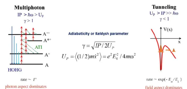
Figure 1.The laser-atom interaction regimes. For adiabaticity parameters larger than unity the photon aspect of the interaction prevails leading to a multi-photon process. For adiabaticity parameters smaller than unity the field aspect dominates, the field modifies the atomic potential forming time dependent (oscillating) barriers and the process is initiated through tunneling or over the barrier ionization.
1.1. Tunneling vs multi-photon
An adequate description of the interaction of intense radiation with matter depends on the interplay between the radiation’s field-strength, carrier frequency and pulse duration, as well as the ionization energy of the matter species. At low frequencies (infrared and lower) and high radiation field-strengths the
atomic/molecular Coulombic potential is severely distorted by the potential of the interaction, and the combined Coulombic and radiation field potentials form a barrier that oscillates with the frequency of the radiation. If the degree of distortion is comparable or larger than the ionization potential, an electron can tunnel through the barrier or escape above it respectively. Since the frequency is low, the potential distortion process is quasi-static and thus the tunneling probability is not negligible. The tunneling rate can be treated, in the appropriate limit, as the DC tunneling ionization rate [5] averaged over a single period of the field.
Here the field aspects dominate the interaction process (figure1right panel). In the opposite side, at not too high field-strengths and high frequencies (ultra-violet, vacuum ultra-violet, x-rays) the degree of the potential distortion is much lower than the ionization potential, the oscillations are much faster and thus the tunneling probability (or over-the-barrier ionization) is strongly reduced. The interaction is now dominated by the photon aspects of the radiation, namely the interaction leads to MP absorption and eventually to ionization (figure1left panel). The ionization rate in that case can be treated through lowest order perturbation theory (LOPT).
The above discussion can be quantified by a parameter known as adiabaticity or Keldysh parameter [6], given by
γ= IP/2Up (1.1.1)
IP being the ionization energy andUpthe so called ponderomotive potential, which is the mean kinetic energy of the oscillation of a free electron interacting with the radiation field
Up= 1
2m˙x2 =e2E20/4mω2 (1.1.2)
withm, xandebeing the mass, position and charge of the electron respectively andE0 andωthe field amplitude and radial frequency respectively.
A practical numerical evaluation formula forUpis:
Up(eV) =9.3·10−14·I W
cm2 ·λ2(µm). (1.1.3)
WhenUp>IP ωthenγ< 1 and the strong field interaction leads to tunnel ionization, while when IP> ω>Upthenγ> 1 and the interaction and ionization has a MP character. It should be noted that we can safely talk about tunneling or MP only ifγ 1 orγ 1, respectively.
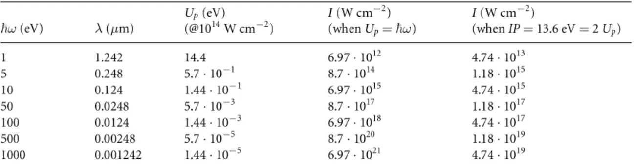
Table 1.Scaling of UPwith the photon energy.
ω(eV) λ(µm)
Up(eV) (@1014W cm−2)
I(W cm−2) (whenUp= ω)
I(W cm−2)
(whenIP=13.6 eV=2Up)
1 1.242 14.4 6.97·1012 4.74·1013
5 0.248 5.7·10−1 8.7·1014 1.18·1015
10 0.124 1.44·10−1 6.97·1015 4.74·1015
50 0.0248 5.7·10−3 8.7·1017 1.18·1017
100 0.0124 1.44·10−3 6.97·1018 4.74·1017
500 0.00248 5.7·10−5 8.7·1020 1.18·1019
1000 0.001242 1.44·10−5 6.97·1021 4.74·1019
Apparently, becauseγis inversely proportional to the wavelength the MP character will be more
pronounced at short wavelengths. Moreover, increasing the ponderomotive potential, via the field’s intensity, has an upper limit set by the depletion of the medium. Indeed, the radiation pulse has a temporal
distribution. Even if intensities could be increased limitlessly, ionization would be saturated at the leading edge of the pulse due to the finite rise time of the radiation pulse. Hence, the medium would never ‘see’ the peak intensity [7] as it would be depleted before the top of the pulse is reached; an effect sometimes referred to as ‘The Lambropoulos curse’ [8,9], because it invalidated as non-realistic several fascinating effects predicted in high intensity laser-matter interactions in the 80 s. The large frequency and limited intensity
‘seen’ by the matter ensure that interactions in the XUV and much more pronounced in the x-ray spectral region, are of MP character.
Table1gives some numerical examples of the scaling of the ponderomotive energy with photon energy.
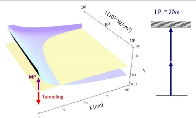
The third column gives the ponderomotive energy at 1014W cm−2intensity. The fourth column gives the intensity at which the ponderomotive shift becomes equal to the photon energy and the last column the intensity at which it becomes equal to half the ionization energy. From table1one can extract that for photon energies≥10 eV,γbecomes < 1 at intensities that the atom/molecule will not be subjected to, unless the interaction is with pulses of very short duration. The role of the pulse duration will be discussed in the next section. In figure2the blue curved surface shows the dependence of the Keldysh parameter,γ, on the wavelength and intensity of the radiation, for the case, where the photon energy is about half the ionization energy. The horizontal flat yellow surface consists of all wavelength-intensity value pairs for whichγ=1. As can be seen in this graph the tunneling regime is safely reached at intensities > 1016W cm−2for 20 eV photons and at higher intensities for larger photon energies. For pulses with durations > 0.1 fs, these intensities are above the atomic/molecular ionization saturation intensity, meaning that the atom/molecule will be essentially fully ionized before the peak intensity is reached. Therefore, one can safely conclude that for photon energies≥20 eV and pulse durations≥0.1fs the interaction is of MP character. However, strong field effects become observable in specific cases at the today’s available FEL intensities [10].
It is worth adding here that the effect of ionization saturation during the raising edge of the radiation pulse is not always a disabling effect. Indeed this effect underlies the temporal gating technique known as
‘ionization gating’ that enables the generation of isolated attosecond pulses [12,13].
1.2. The ionization of an atom/molecule. ‘Coring’ vs ‘Peeling’
The intricacies of ionization upon interaction of short wavelength radiation with matter are governed by the ratio of thephoton energyoverionization energyof the first inner shell of the matter.
If this ratio is > 1 an inner shell electron is ejected with notably higher probability than an outer one (a process frequently referred to as ‘coring’) leaving an inner shell hole behind. The hole is eventually filled, in the vast majority of the cases, through an Auger or Coster–Kronig process [14], producing a doubly ionized atom/molecule. Absorption of subsequent photons leads to repetition of the process described, as long as the above mentioned ratio is larger than unity. High charge state ions are thus produced through a sequence of single photon absorption processes (and eventually subsequent relaxation processes), each of which leads to the next charge state of the ion.
The photo-ejection of an inner-shell electron discussed here theoretically can also proceed via MP absorption. However, in order for this process to compete with the ejection of an outer electron, a challenging combination of pulse duration and energy, not available in any laboratory or research infrastructure so far, is required. Thus ‘coring’ processes are so far sequences of single photon absorption events (sequential coring). In contrast, for a ratio < 1 an outer shell electron is ejected leaving a singly ionized ion behind and absorption of further photons leads to the ejection of additional outer electrons provided that the ejection is energetically allowed (a process frequently referred to as sequential peeling). Under specific conditions, ejection of two electrons leads to a doubly ionized ion without intermediate production
Figure 2.Adiabaticity parameter as a function of wavelength and intensity for ionization energies of about two times the photon energy. The horizontal yellow plane is the border between multi-photon and tunneling regimes. Given that a two-photon ionization saturates at about 1015W cm−2[11], for the wavelength region shown here the ionization process is always multi-photon (two-photon).
of a singly ionized ion, a process known as direct double (or multiple) ionization. An inner shell non-linear process, i.e. absorption of more than one photons by one or more inner shell electrons leading to some stage of ionization, without formation of intermediate charge states, is currently not possible, since it requires very short pulse durations at high pulse energies, a matter that will be discussed in the next section. Such a process can currently be considered only as a future perspective. On the contrary multi-XUV-photon absorption by outer electrons is feasible at the currently available XUV intensities in FEL infrastructures as well as in laser driven HHG [15,16] sources. This has led to the revitalization of MP processes, a forefront research topic at optical frequencies in the 70 s, 80 s and 90 s, now in the XUV/x-ray regimes.
1.3. The era of non-linear XUV processes, their contribution in attosecond metrology and science Historically, MP processes trace back to the 30 s. It was Maria Göppert Mayer who first predicted
two-photon processes, talking about ‘two quanta jumps’ (Über Elementarakten mit zwei Quantensprünge”) [17]. About 30 years later, in the 60 s, the invention of the laser led to the first experimental observation of MP processes [18,19]. Another 30 years later, in the 90 s, the development of intense laser HHG sources [20,21] led to the first experimental observation of multi-XUV-photon processes [22]. The importance of observable multi-XUV-photon processes relates to a number of advanced applications.
Concerning applications in temporal pulse characterization, non-linear XUV processes hold promise for rigorous attosecond pulse reconstruction. The most frequently used methods for the temporal
characterization of fs pulses are based on non-linear processes both in the time domain, like second- and higher-order autocorrelation, frequency resolved optical gating (FROG) [23], attosecond spatial
interferometry [24] or in the frequency domain like Spectral Phase Interferometry for the Direct Electric Field Reconstruction (SPIDER) [25] to mention some. In attosecond pulse metrology, due to the lack of sufficient pulse energy, a number of cross-correlation (infrared (IR)/XUV) techniques have been developed such as Reconstruction of Attosecond Beating By Interference of two-photon Transitions (RABBIT) [26], Frequency Resolved Optical Gating for Complete Reconstruction of Attosecond Bursts (FROG-CRAB) [27], Phase Retrieval by Omega Oscillation Filtering [28],in-situ[29], atto-clock [30], double-blind holography [31] and the attosecond streaking [32] methods. A summary of these approaches can be found in the perspective article on the attosecond pulse metrology [33]. Non-linear XUV processes allowing the
performance of second-order autocorrelation based techniques relying solely on the XUV radiation provide an alternative attosecond pulse characterization approach bypassing possible inconsistencies inherent in the other methods [34]. Still, robust utilization of non-linear XUV processes in attosecond pulse
characterization is subject to the availability of sufficient stability of the XUV radiation parameters and high repetition rate sources.
Applications in the investigation of ultra-fast dynamics using attosecond pulses follow similar pathways.
Cross-correlation (IR/XUV) approaches like RABBIT, RAINBOW RABBIT [35] and attosecond streaking have been successfully used in numerous fascinating applications; atomic inner-shell spectroscopy [36], real-time observation of ionization [37], light wave electronics [38] and molecular optical tomography [39,40] are some examples of such experiments. Other more recent applications of attosecond pulses include ionization delay in solids [41] and atoms [36,37] and molecules [42,43], electron dynamics [44], charge migration [45,46], build-up of a Fano-Beutler resonance [35], ionization dynamics in chiral molecules [47], to mention some from the very many. Alternatively, non-linear XUV processes allow conducting
XUV-pump-XUV-probe experiments with sub-fs temporal resolution overcoming complications, that may arise in some cases in conventional IR/XUV pump-probe experiments, related to distortions suffered by the system under investigation due to the IR laser/matter interaction that may obscure the intrinsic dynamics of it [48]. XUV-pump-XUV-probe schemes involve at least two-XUV-photon processes and thus non-linear XUV processes offer an advantageous tool in attosecond metrology.
An additional advanced application of non-linear XUV processes arises from the spatial selectivity they provide. Since the non-linear process becomes observable at high intensities and thus in focused beams, the focal area provides spatial selectivity allowing 3D mapping of a sample. Spatio-temporal resolution (4D) may reach the sub-µm and attosecond regimes.
Attosecond pulses as coherent pulses allow frequency domain Ramsey spectroscopy type of
measurements [49–51] as well. The superposition of two mutually delayed attosecond pulses result in a modulated broad frequency spectrum. Variation of the delay between the two pulses translates to a variation of the position of the frequency peaks. The distance of two consecutive frequency peaks is inversely
proportional to the delay of the two pulses. This allows frequency domain measurements the frequency resolution of which is increased when two-XUV-photon transitions are involved coupling narrow spectral width metastable states.
Nonlinear XUV spectroscopy could also be considered an important tool for the validation of numerical models for the description of electronic correlation in atoms and small molecules. In this research direction, the process of two-photon double ionization represents an ideal benchmark. When confined to the
attosecond timescale, the correlated electronic dynamics should be manifested in the relative angular distribution of the photoionized electrons [52]. Such an experiment still represents a formidable technological challenge for nonlinear XUV spectroscopy as it would require the combination of
high-intensity XUV pulses, attosecond pulse durations (and control of relative delay between two pulses on a similar timescale) and high-repetition rate sources (for the coincidence characterization of the
two-photoelectrons). Even though preliminary, partial experimental data on double ionization of helium and neon were obtained at FLASH [53,54], there are several characteristics of the process that still need to be investigated.
Non-linear XUV processes made their debut some 20 years ago. Limitations preventing their earlier observation relate to the high intensity they require, while their utilization in applications was hampered since they are inherently absorbed by any material. The latter restriction further prohibits the use of refractive optical elements in the experimental set-ups.
High intensity limitations relate to the low throughput of gas target HHG sources and XUV optical elements, while an additional restriction arises from possible reabsorption of the XUV radiation at the source itself. Limitations on the throughput of gas target HHG sources originate from the depletion of the
generation medium, which at a given intensity is fully ionized and no medium emitters remains to generate harmonics. Since HHG relies on the interaction of matter with an IR pulse, even if very high laser pulse energies are available ionization will saturate at the leading edge of the laser pulse once the ionization saturation limit is reached. The emitter will be fully ionized and thus the higher intensities will not be ‘seen’
by the depleted generating medium. Moreover, in the created plasma the index of refraction at a given angular frequencyω, nω≈1− ω
2 p
2ω2 is determined by the plasma frequencyωp=e mεNe
0, withNethe electron’s density andε0the vacuum permittivity. Saturation of ionization will result to a large electron densityNeleading to negative dispersion that may destroy phase-matching.
Reabsorption of the XUV radiation at the source sets additional limitations in the generation medium length and atomic density. The absorption length in the generation medium is given byLabs≈(σNa)−1, whereσis the absorption cross section andNathe atomic density. Therefore, increasing the medium length or the gas pressure such thatLabsNa> σwould be meaningless as reabsorption would prevent an increased throughput. Mitigation strategies of medium depletion and reabsorption are described in section2.
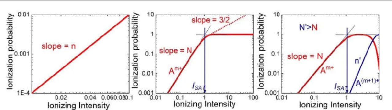
Figure 3.LOPT ionization probability of n-photon non resonant ionization in log-log scale. Below saturation the plot is a straight line with slope n, the degree of non-linearity of the process (left panel). At saturation the probability becomes 1 and eventually drops because ionization of the singly ionized species sets in (center panel). Inclusion of the spatial distribution of the radiation results to a strongly modified slope above the saturation regime, independent on the non-linearity degree of the process (right panel).
Other source throughput limitations are raised by the necessity to use only reflection optics in steering, focusing or splitting the XUV beam, because XUV radiation is highly absorbed when it propagates in matter.
This point will also be discussed in section2.
1.4. MP ionization yields and the required XUV intensity and pulse duration parameters
In an-photon non-resonant ionization process the time evolution of the ionization probabilityP(t) can be described by the rate equation:
dP(t)
dt = (1−P(t))σ(n)Fn(t) (1.4.1)
where
Fn(t) =I(t)
ω =F0f(t) (1.4.2)
is the photon flux,I(t) the intensity envelope,F0the instantaneous peak photon flux,ωthe angular frequency,f(t) the temporal pulse profile withf(t=0)=1 andσ(n)the generalizedn-photon ionization cross section usually given incm2nsn−1so that the ratedP/dtis given in s−1when the intensity is given in W/cm2.
Defining an effective timeteff= ∞∫
−∞fn(t)dt integration of (equation1.4.1) yields an ionization probability at the end of the ionizing pulse:
P(t→ ∞) =1−exp −σ(n)Fn0teff . (1.4.3) Below saturation of ionization, i.e. whenσ(n)Fn0teff 1
lnP(t→ ∞) =nlnF0+lnσ(n)+lnteff. (1.4.4) Thus, the ionization probability depends linearly on the photon flux (or intensity) in log-log scale below saturation, with a slope equal to the degree of the non-linearitynas shown in figure3(left panel). Including saturation and defining the ionization saturation intensity as
ISAT= √n ω
σ(n)teff,the ionization probability at the end of the pulse becomes P(t→ ∞) =1−e− ISATI
n
(1.4.5) and forI ISATreduces toP(t→ ∞) = ISATI n=σ(n)Fn0teff. A plot of (equation1.4.5) in log-log scale is shown in figure3(right panel). AsIapproachesISATthe increase of the probability slows down and at saturation becomes 1. Above saturation (I>ISAT) the probability drops because the ionization of the singly ionized species sets in.
It should be noted that because the ionization radiation at the focus has a 3D intensity distribution I=I(x,y,z) the ionization probability will also have a spatial distributionP=P(x,y,z) and even if the central part of the interaction volume is saturated the surrounding will not be. When the ionization probability
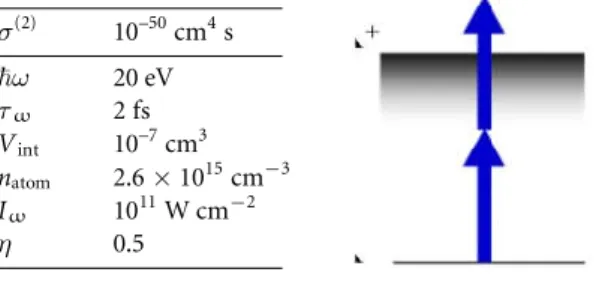
Table 2.Typical two-XUV-photon ionization parameters.τωdenotes the duration of the XUV pulse.
σ(2) 10–50cm4s
ω 20 eV
τω 2 fs Vint 10–7cm3 natom 2.6×1015cm−3 Iω 1011W cm−2
η 0.5
measurement is not spatially confined, but it is integrated for the entire interaction volume the probability P(t→ ∞)´ ´ ´
p(x,y,z)dxdydz=´ ´ ´ I(x,y,z)
ISAT dxdydzwill neither stabilize at unity nor drop at and above the saturation intensity respectively. It will continue increasing due to the volume integration.
For a Gaussian distribution in cylindrical coordinates the spatiotemporal intensity distribution is I(r,z;t) =I(t) w20
w(z)2exp − 2r2
w(z)2 (1.4.6)
whereris the radius,zis the beam propagation axis andw(z) is the beam radius, defined in terms of the beam waistw0asw(z) =w0 1+ (z/zR)2. The ion yields can then be integrated using the expression
P(t→ ∞) =rmax∫
0 zmax
zmin∫
2πrP(r,z)dzdr (1.4.7)
whereP(t→ ∞)is the integrated over the volume ionization probability at the end of the pulse andP(r,z) the ionization probability at each point (r,z). Above saturation, (equation1.4.7) results to a line with a slope of 3/2 as shown in figure3(middle panel). This effect known as the ‘volume effect’ can be eliminated by a spatially confined measurement of the ions as will be discussed in section2.
The generalizedn-photon ionization cross section in the electric dipole approximation within the LOPT reads:
σ(n)∝ i1. . . i1 g|rˆe|i1 . . . in−1|rˆe|f +∫dε g|rˆe|ε ε|rˆe|f Ein−1−Eg−(n−1) ω . . . Ein−1−Eg− ω
2
(1.4.8) where|g,|f ,|ik(k=1,…n-1) and|ε >are the ground, final, all electric dipole allowed intermediate bound states involved and all electric dipole allowed continuum states involved respectively.Eg,Ef,EikandEare the corresponding eigenenergies,ris the electron position operator andˆethe electric field polarization unity vector.Ab initiocalculations ofσ(n)are feasible for some atoms for which the eigenstate wave functions can be deduced from the Schrödinger equation when exact or accurate atomic potentials are available, as for instance for H and He atoms [55]. In general, generalized ionization cross section can be calculated to some degree of approximation. However, good estimates ofσ(n), sufficient to describe the essential features of the process, can be obtained from the corresponding cross section of Hydrogen atom using scaling laws [56,57].
Based on the above discussion one can estimate the required XUV intensities in order to achieve
observable two-XUV-photon ionization, i.e. the lowest possible non-linear ionization process. The measured number of ionsNIonper pulse will be given by
NIon=P×Vint×natom×η (1.4.9)
where P is the ionization probability,Vintthe interaction volume,natomthe target atomic (/molecular) density andηthe detection efficiency of the measuring device. Typical values of the above quantities are summarized in table2. These parameters resultNIon=2–3 ions/pulse. Thus, intensities of 1011W cm−2are at the limits of observable two-XUV-photon ionization. Intensities≥1012W cm−2are required for reliable two-XUV-photon ionization intensity dependence experiments.
In large pulse duration interactions ionization yields are enhanced if the process is resonant with one (or more) of the eigenstates. Large pulse duration here means that the duration is comparable or larger than the lifetime of the state, when decaying through spontaneous emission. For a two-photon resonantly enhanced ionization by a bichromatic field the ionization rate becomes
P= ∞∫
−∞σ1×F1dt× ∞∫
−∞σ2×F2dt= σ1×σ2
∞∫
−∞
I1
ω1
dt× ∞∫
−∞
I2
ω2
dt (1.4.10)
Table 3.Typical two-XUV-photon resonantly enhanced ionization parameters. Two XUV frequencies are assumed. The first being resonant with the transition frequency from the ground to the excited state and the second one is in general different than the first one.
τi(i=1,2) are the pulse durations of the two XUV frequencies, which are assumed to be equal.
σ1×σ2 10–34cm4
ω1,2 10 eV
τ1,2 2 fs
Vint 10–7cm3 natom 2.6×1015cm−3 I1,2 1011W cm−2
η 0.5
withσi(i=1,2) being the single photon absorption cross sections of the two steps andFi,Ii,ωithe photon fluxes, intensities and angular frequencies of the two fields, respectively. Using typical values for all the quantities (e.g. those of table3) one can evaluate the number of generated ions per pulse from (equation 1.4.9) to beNIon≈2500 ions/pulse, which is three orders of magnitude larger than in the non-resonant.
In obtaining the above number of ions we used as the effective duration of a Gaussian pulse τeff = ∞∫
−∞e− 2τ1,2t
2
dt=3.5τ1,2. However, for the evaluation of the ion yield here, no account is taken that from the broad spectrum of the radiation pulse only the part that corresponds to the state width is resonant and thus only this fraction should be used from the initial intensity (1011W cm−2).
Ionization by the two parts of the spectrum lying above and below the resonance will cancel due to the opposite detuning and thus to the opposite phases of the corresponding ionization pathways. Taking this into account for bound states with lifetimes of the order of 1 ns, the resonant channel of the ionization becomes negligibly small compared to the non-resonant channel. For this reason, for very short pulses in the attosecond and few fs temporal regime the resonant character of the process is lost unless the lifetime of the state is comparable to the pulse duration as is the case for fast decaying autoionizing states (AIS). In this case the resonant character will be present and may enhance the yield. The situation may become more complex if the experimental parameters become such that the population of the resonant state becomes comparable to the remaining population in the ground state. In such cases the ionization yield may be enhanced. Under such conditions the problem is treated more accurately as described in the following paragraphs and even better if it is solved numerically, since then parameters, such as the width and position of the resonant state, are becoming time dependent.
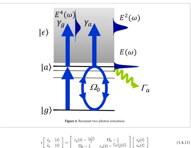
Rigorously, the problem should be treated through the time dependent Schrödinger equation (TDSE) and not through rate equations. In solving the TDSE for the case of a two-photon ionization it is assumed that the system is initially in the ground state, |g (energyEg), subject to a radiation field E(t) with a central-carrier frequency,ω, which is near resonant with an excited state |a> (energyEa).
The atom can be ionized through two different ionization channels; (a) by absorbing two photons non-resonantly (direct channels) and (b) via the excited state, following the absorption of one-photon and ionization from further photon absorption (sequential channel). However, the atom, once found in the excited state can also be de-excited back to its ground state by photon emission. The photoionization scheme is depicted in figure4.
The TDSE is solved by first transforming to a slowly-varying-amplitude (SVA) [58] system and then applying the rotating wave approximation (RWA) [58,59] on the amplitude equations for the ground and the excited state, i.e. eliminating the resulting high frequency terms [(Ea-Eg)/ +ω] keeping terms oscillating at [(Ea-Eg)/ –ω]. It is worth emphasizing that the change to a system of SVA variables does not involve any approximation and as such the transformed TDSE is still exact in the context of a two-level system
interacting with a laser field. The applied transformation effectively extracts the fast-oscillating part of the amplitude coefficients due to the energy difference of the two states ~(Ea- Eg) (also known as the interaction picture). The SVA transformation combined with the RWA results in expressing the TDSE in terms
exclusively of slowly-varying variables, namely, the field’s envelope and the periodic ~ exp(i(Ea-Eg)/ –ω)/t]
factor. The corresponding (strongly-oscillating) term ~[(Ea-Eg)/ +ω] is discarded. This method is effective if i) it can be modeled in factors of an envelope-like amplitude E0(t) and a periodic term oscillating with a central carrier frequency e.g. ~E0(t)×cos(ωXUV×t); for the latter assumption a quantitative condition is dE0(t)/dt ωXUVE0(t), which generally holds for a few fs pulse with central frequency in the XUV regime and ii) as long as the field is not extremely intense so thatΩ0 ωXUV,Ω0being the Rabi frequency. The transformed amplitude equations for the ground and the excited state now obey the following
coupled-system of differential equations,
Figure 4.Resonant two-photon ionization.
i ˙cg (t)
c˙a (t) = εg(t)−γg2(t) Ω0−2i
Ω0−2i εa(t)−Γa+γ2a(t)
cg(t)
ca(t) (1.4.11)
whereq=√2Ωγg0γa,εi(t) =Ei+si(t),i=g, aandcg(t),ca(t)the time dependent state amplitudes, i.e. the square root of the probability to find the system in the corresponding state at timet. In these relationssg,sa
andγg, γaare the light shifts, i.e. the shift of the energy of the atom/molecule states induced by the radiation and the widths of the states.Γais the ionization width of the excited state due to other decay channels (e.g.
autoionization). Therefore, the dynamic energiesεg, εahave incorporated the ac-Stark shifts; also the q-parameter describes the interference between the resonant (sequential) and the non-resonant (direct) ionization channels (similar to the traditionalq- Fano parameter). In the above form of the TDSE, all quantities, butΓa, are (non-oscillating) time-dependent quantities varying with the field’s envelope,
sg(t) =sgI20f4(t), γg(t) =γiI20f4(t) (1.4.12) sa(t) =saI20f4(t), γa(t) =γaI20f4(t) (1.4.13) Ω0(t) = Ω0f(t),Ω0(t) =1
2dgaE0f(t) (1.4.14)
wheref(t) is the field’s normalized envelope andI0=|E0|2/4 . The above system of equations results in a time-dependent ionization probability:
P˙(t) = √γgCg+√γaCa 2
(1.4.15) (in density matrix notationγgρgg+γaρaa+2√γgγaRe ρga , the diagonal matrix elements ofρgg, ρaabeing the state amplitudes, i.e. the square root of the population of the states g and a respectively, and the non-diagonal matrix elementρgabeing the so called coherence that relates to the induced dipole moment).
Note that for the ac-Stark shifts, in the range of intensities where the RWA is applicable, the following inequalities apply: sg εgandsa εa. The reason for this resides in the structure ofsgandsaquantities; the numerator is positive while the denominator is positive up to a certain value and then becomes negative, thus amounting to a reduced value due to mutual cancellations.
Solutions for the amplitudes.
In the general case the TDSE system should be solved numerically, especially in the case where all involved parameters are of comparable magnitude i.e. detuning, decay widths, Rabi frequency. Nevertheless, an
approximate analytical expression for the state amplitudes and the ionization is possible for a many cycle field; the general solution for the amplitudes takes a very simple form, as a linear combination of exponentials:
cg(t) =eiˆδt/2 Ωˆ
Ωˆˆs+(t)−∆ ˆˆ s−(t) (1.4.16)
ca(t) =Ω0
Ωeiδt/2ˆ ˆs−(t) (1.4.17)
where all the quantities with hats are complex numbers and determined by the generalized Rabi-frequency, the effective ionization widths and the dynamic detunings,
ˆs±=1
2 eiΩt/2ˆ ±e−iΩt/2ˆ , Ω =ˆ ˆδ2+4Ωˆ02 (1.4.18)
Γ =γa+ Γa+γg, γ=γa+ Γa−γg (1.4.19)
∆ =δ+iΓ
2 ,δˆ=δ+iγ
2 (1.4.20)
Ω0= Ω0 1−i
q (1.4.21)
δ=εg+ω−εa. (1.4.22)
In the general case whereΓais present, ionization may be calculated by,
P(t) =1− Cg(T)2− |Ca(T)|2e−Γa(t−T) (1.4.23) whereTis the interaction time (e.g. the pulse duration). The expression when only photoionization is present is calculated to be,
P(t) =1−e−Γt/2
|ˆs+|2+
∆2+ Ω0 2
Ω2 |ˆs−|2+2Re
δˆ∗Ω
Ω2 ˆs+ˆs−
. (1.4.24)
In all the cases below one can check the role of the interaction time (pulse duration),T, in the observed yields in addition to the role of the ionization widthγ, Rabi-frequency,Ω0, and the detuningδ.
1.5. Resonant caseδ 0and no direct-channel (γg=0) (strong-field)
In this case all quantities become real and the expression for the amplitudes take a very simple oscillatory form. Since,
Γ =γa=γ, 1/q= 0, Ω = 4Ω20−(γ/2)2 (1.4.25) assuming the strong-field case where 4Ω20>(γ/2)2one easily can arrive to the expressions,
cg(t) =2Ω0
Ω e−Γt/4sin Ωt
2 +ϕ (1.4.26)
ca(t) =i2Ω0
Ω e−Γt/4sin Ωt
2 (1.4.27)
with the phase-lagϕdefined as,tanϕ=2Ωγ (cosϕ=4Ωγ
0 andsinϕ=2ΩΩ
0) .Note that the phase-lag between the ground and the excited state is determined by the ratioΩγ0. In this case the ionization probability is given by,
P(t) =1−4Ω20
Ω2 e−γt/2 1− γ
4Ω0cos(Ωt−ϕ) . (1.4.28)
Therefore, the ionization probability is purely oscillatory with a period determined by the generalized Rabi frequency. In the ‘weak’-field case (4Ω20<(γ/2)2) the results are obtained if one setsΩ→iΩ, and the oscillatory functions become purely exponential.
1.6. Strong and short pulse (γ,Γ Ω0andγT,ΓT 1)
In this case where both the direct- and the sequential channels are present the following expression for the ionization rate can be derived,
P˙(t)∼= γa 4Ω02
δ2+4Ω02sin2Ωt+γg+2qγaγg δ
δ2+ Ω02sin2Ωt. (1.4.29) If the interaction time is much larger than the Rabi’s period (|Ω|t 1) then integration of the above time-dependent ionization probability provides an ‘average’ ionization rate, which resembles a Fano-profile placed on a constant background (of the direct ionization channel).
1.7. MP multiple ionization
When the intensity is sufficiently high multiple ionization may occur involving i) sequential processes where all intermediate charge states get populated and the next charge state is reached through photon absorption by the previous populated charge states, ii) direct processes in which two or more electrons are ejected without formation of the lower charge states and iii) processes populating excited bound or AIS of the ionic stages. Thus, different channels can contribute to the formation of a certain charge state. The temporal evolution of the processes involved can be described through rate equations from which the ionization probability can be evaluated.
At this point, it should be made clear that the most general treatment of the ionization processes should involve the density matrix formulation for all possible states of the combined atom and laser system with both the coherent (relative atomic amplitude’s phases are important) and incoherent processes incorporated on an equal footing. Additionally, the density matrix is a statistical approach appropriate not only for pure states but also for mixed states, i.e. ensembles of which we only know their statistical distribution. In this sense the TDSE and the rate equations have a different validity range of parameters, in fact they are placed on opposite sides. When the relative atomic phases are unimportant then one can obtain a simplified model of the ionization process, that of rate equations. In the opposite case, i.e. the case when the relative atomic phases cannot be ignored, the TDSE formulation can be used in order to describe an ionization process; thus it represents the other ‘simplified’ extreme (treating only pure states and only partially decoherence
phenomena) where the relative phases are crucial for the system’s dynamics. However, for the latter case TDSE is only nominally a simplified system of ‘equations-of-motion’ since all the excited (bound and continuum) atomic states in principle should be included. Nevertheless, a simpler form can be obtained under certain conditions involving amplitude equations, of the same type as discussed in the two-level system model earlier. In all of its full generality, the TDSE system can be solved very accurately only for the lighter atomic systems, such as the hydrogen and helium. For all other atomic systems more drastic approximation models are used, especially when multiphoton processes contribute to the excitation and ionization. One may loosely say that the rate equations treat the ionization process in an ‘averaged’ fashion thus ignoring any phase relationship between the atomic states (bound or excited). The state’s population are the main actors in this model. The SVA and the RWA are applied into the TDSE with the additional
assumption that the relative phases follow adiabatically the populations of the atomic states. Eventually, the ionization process is described by a single absorption rate, via the (multiphoton) ionization cross section.
Therefore, any resonance features are only implicitly incorporated in the values of the cross section for the given field’s frequency. This particular approximation gradually loses its meaning as the spectrum of the field broadens (or equivalently the pulse shortens) since the cross sections are, in principle, meaningful quantities only for monochromatic pulses. Hence, one may not hope to fully replicate the results either of a model based on a full density-matrix or TDSE formulation but only to estimate ionization rates for experimental schemes which meet the physical conditions set above. The resulting rate equations have the structure of a system of ordinary differential equations which normally may be calculated without complications. This is the task of the rate equations model as it, very nicely, factorizes the ionization process into its main
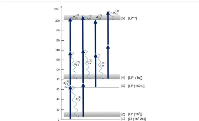
Figure 5.Multi-photon ionization of Li by pulses with a central photon energy of 68 eV. Only lowest order channels leading to a given final state are considered.
constituents: the states’ population,Ni, the field part via its fluxF(t) and their interaction strength through the various cross-sectionsσab. The formidable task is the calculation of the cross sections rather than solving the rate equations. The structure of the rate equations is such that the total rate of the system sums to zero as one should expect from a population-transfer modeling, a model which in other fields is not the exception but the rule e.g. in biology, chemistry, statistics etc. Computationally, the rate equations’ approach is by far the less demanding one, followed by the TDSE. The reader interested in a more extensive account of the rate equations ionization model could find it in the classic text by Shore [60].
To give an example of a simple system, assume ionization of Li atoms by a pulse of 1fs duration with central photon energy 68 eV and a peak intensity of 1015W cm−2. The equations of motion for the Li charge states following ionization from the ground state by a pulse with central frequency at 68 eV are given below:
Li 1s22s dN1
dt =− σ(1)12 +σ(1)13 F(t) +σ14(2)F2(t) +σ15(3)F3(t) N1 (1.4.30) Li+ 1s2 dN2
dt =σ12(1)F(t)N1− σ(2)24F2(t) +σ(3)25F3(t) N2 (1.4.31) Li+(1s2s)dN3
dt =σ13(1)F(t)N1−σ(1)34F(t)N3 (1.4.32) Li2+(1s)dN4
dt =σ(2)14F2(t)N1−σ45(2)F2(t)N4+σ24((2))F2(t)N2 (1.4.33) Li3+dN5
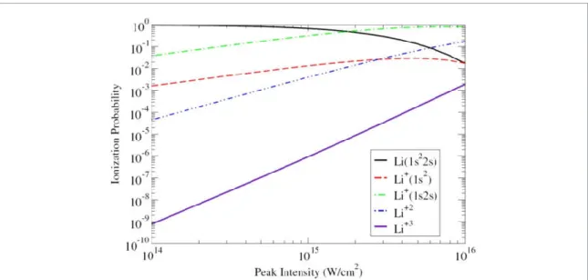
dt =σ25(3)F3(t)N2+σ(2)45F2(t)N4+σ((3))15 F2(t)N1 (1.4.34) whereF(t)=I(t)/ ωis the field’s flux andσ(n)ij the generalized cross sections for the respective ionization processes. The order of the cross sections is denoted in parenthesis and is equal to the flux’s appearance power. The various pathways are depicted in figure5while the ionization yields for the given pulse are plotted in figure6.
It should be noted that, although the channel to the Li+(1s2p) continuum is energetically open through electron-electron correlation, it is much weaker (~15 times weaker than the channel to Li+(1s2 s)) and thus has been neglected. Also, the two-photon ejection of two electrons from the Li+1s2 s state (transition |3 →
|5 ) has been neglected because this channel is open to only a small part of the bandwidth of the radiation.
Figure 6.Ionization yields of all Li charge states as a function of the ionizing intensity.
The field’s intensity is modelled byI(t) =I0e− t/
τ 2, whereτis related to the effective pulse duration. The main difficulty in solving the above system of rate equations resides in the calculation of the atomic parametersσijsince generally several of them have not been yet calculated with a rigorous calculation method. These are then estimated based on scaling properties of atomic systems as well as properties related to the nature of the electromagnetic field interaction. In the present case the following values have been chosen for the calculation of the ionization yields:σ(1)12 =10–19cm2;σ13(1)=2·10−18cm2,σ(2)14=10–53cm4s;
σ(2)24=10–51cm4s;σ35(2)=10–53cm4s;σ34(1)=10–19cm2;σ45(2)=10–53cm4s;σ25(3)=10–87cm6s2and σ(3)15=10–87cm6s2.
As it is beyond the scope of the present work to describe the calculation details we delegate the interested reader to other more elaborate works for this task [61,62] (and references therein). A package for the ab-initiocalculation of one-and two-photon cross sections of two-electron atoms, using a configuration interaction (CI) B-splines method can be found in [63]. There is a large number of publications involving rate equations of two- (or few-) photon ionization. The ‘simplest’ case is He for which a study in the photon energy range 45–54 eV can be found in e.g. [64]. In case of more complex systems and more photon ionization cases the number of rate equations increases significantly [65].
There are many publicly available packages for numerical calculations in atomic and molecular systems such as, the COWAN package [66], BSR [67], BSPCI2E [63], QPROP [68], RMT [67], and the quantum chemistry packages UKRmol [69] and MOLPRO, to mention a few; but, due to the highly specialized numerical approaches, the codes are mostly developed and used in-house.
The above discussion and parameters concern multi-XUV-photon absorption by an outer shell electron, which are processes that have been realized utilizing initially individual harmonics of laser radiation and later on radiation of FEL sources, as well as laser based attosecond-pulse sources. Apart from sequences of single photon inner-shell absorption processes leading to multiple ionization, two- or more XUV photon
absorption by an inner-shell electron has not been demonstrated yet. This is attributed mainly to the lack of the required experimental parameters that would allow such a process to compete with lower linear processes of the outer shell electrons. In order to estimate such experimental parameters, cross sections of two- (or multi-) photon inner-shell ionization are required. Good estimates of two-photon K-shell cross-sections can be calculated for hydrogen-like ions using scaling. For a two-photon ionization (equation1.4.8) reads
σ(2)∝ω2 ι1 g|rˆe|ι ι|rˆe|f +∫d g|rˆe| |rˆe|f Eι−Eg− ω
2
. (1.4.36)
Continuum renormalization ε|ε = δ(E−E)results in |f ,|ε ∝Z−1,Zbeing the charge of the nucleus of the hydrogen-like ion. Thus, the matrix elements anddεin (1.4.36) scale with Z like:
g|r|i ∝Z−1, i|r|f ∝Z−2, g|r| ∝Z−2, |r|f ∝Z−3 (1.4.37)
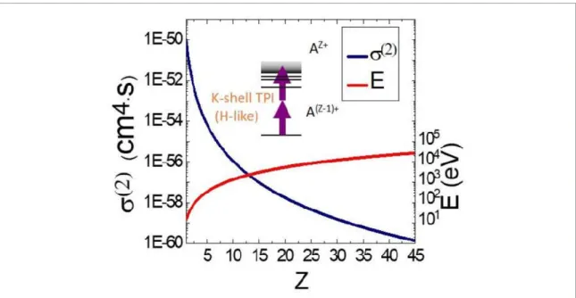
Figure 7.Generalized two-photon ionization cross sections and ionization energies of hydrogen-like ions.
and
d ∝Z2. (1.4.38)
Hence, the cross section
σ(2)(Z, ω) = 1
Z6σ(2) Z=1, ω
Z2 (1.4.39)
drops dramatically for heavier ions.
Figure7shows the Z dependence of a two-photon K-shell ionization generalized cross section of hydrogen-like ions and the corresponding photon energy threshold at which the two-photon ionization channel opens. Due to theZ−6dependence of the cross section, in order for the two-photon ionization process of the inner shell to compete with the single photon ionization of the outer sell at intensities lower than the ionization saturation intensity, the pulse duration has to be extremely short. To give an example, for Z=4 (beryllium atom) and photon energy 110 eV, approximating the two-photon K-shell ionization of the atom with that of the hydrogen-like ion of the same Z, the two photon generalized cross section becomes σ(2)K=5·10−54cm4·s. The L-shell single photon ionization cross section isσ(1)L~ 10–20cm2. For a pulse duration of 40 asec the two-photon K-shell ionization will become the dominant process at intensities larger than 5·1016W cm−2, while ionization saturation occurs at ~1018W cm−2. Therefore, for a large interval of intensities, ionization will essentially occur via two-photon K-shell absorption.
For a pulse duration of 1 fs, two-photon K-shell ionization becomes comparable to the L-shell single photon ionization just before saturation sets in. It becomes obvious that energetic attosecond pulses are required in order for the process to become observable. For the time being, even for the relative low Z of our example, the parameters discussed are not available in any currently operational XUV source. Nevertheless, they are close to become available in the near future. However, when going to higher Z the parameters become extreme. To give an example, for neon intensities of the order of 1020W cm−2and pulse durations of the order of 10 asec, are necessary.
It is worth noting that (equation1.4.1) is rigorously valid only if the field is fully coherent i.e. if its quantum state is the coherent sate of light. For any quantum state of light, the ionization probability rate is
dP(t)
dt ∝σ(n)G(n) (1.4.40)
whereG(n)is the n-th order intensity correlation function of the field. For the coherent state of light G(n)∼= Nn,Nbeing the photon number and thus (1.4.40) reduces to 1.4. For the chaotic state of light (thermal light)G(n)∼=n! Nn, and for a photon number squeezed state of lightG(n)∼= (2n−1)!!N n [70–72]. Thus, at first glance and kind of counterintuitively MP ionization by chaotic light is more efficient than by coherent light. However, if one realizes that in chaotic light, the photons are statistically more
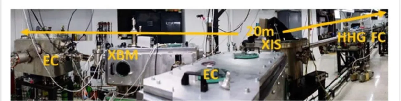
Figure 8.The 20GW HHG beamline of the attosecond science and technology lab of FORTH. EC: Experimental chamber; XBM:
XUV Beam Manipulation chamber; XIS: XUV-IR separation chamber; HHG: High Harmonic Generation chamber; FC: Focusing Optics chamber.
‘bunched’ than those of a coherent light, this observation is of no surprise. This is experimentally verified already in the 70’s [73] and recently in a more controllable way [74]. This dependence of the efficiency of MP processes on the quantum state of the light may lead to differences in experiments conducted at FELs and XUV sources based on the process of HHG by lasers [11].
2. Experimental methods for non-linear XUV optics
As stated in the introductory section we address mainly laser-driven tabletop XUV sources. In this section we focus on methods and instrumentation dedicated to the investigation of non-linear XUV processes
exploiting such sources. Several of the methods and instrumentation coincides with those used in FEL infrastructures. Methods and instrumentation that are exclusively used in FEL facilities are beyond the scope of this manuscript and thus will not be addressed here.
2.1. High photon-flux laser driven, tabletop XUV sources based on harmonic generation in gas targets Laser-driven attosecond sources are based on HHG ([20,21] and references therein). Harmonic generation is a highly non-linear process and consequently its throughput is drastically increased with the driving intensity and more precisely with the order of non-linearity, which is between 4 and 5 [75–77]. As mentioned in section1.3, the main obstacles in reaching the high XUV photon fluxes, required for inducing non-linear XUV processes in laser based attosecond sources using gas targets as non-linear media are the depletion of the generating medium, the phase mismatch due to plasma formation and the XUV radiation reabsorption by the generating medium itself. Partial mitigation of these limitations, leading to a higher source throughput, is to drive the harmonic generation process using long focal length optical elements to focus the laser in the medium. In this way the cross section of the laser beam in the interaction region increases and thus a higher number of emitters and photons contribute to the generation while ionization remains below saturation.
When a small length medium in comparison to the confocal parameter is used, as is the case when pulsed nozzles are employed, the interaction length remains effectively unchanged when the focal length is
increased. When a large length medium, as compared to the confocal parameter is used, as is the case when long cells are used, increasing the focal length will increase the interaction length and the product LabsNawill became larger thanσ. Reabsorption will then prevail. In this case the gas pressure must be decreased such that the product will remain smaller thanσ. A detailed investigation of the scaling of the source parameters focal length, laser field and atomic density can be found in [78].
An implementation of large focal length (9 m) gas jet source is the 20 GW XUV beamline of the Attosecond Science and Technology lab of the Foundation for Research and Technology, Hellas (FORTH) (figure8). Using Xe as harmonic generating medium a maximum XUV pulse energy of the order of 200µJ in the spectral region 15–30 eV has been demonstrated [11]; more recently a train of pulses with sub-fs pulse durations have been measured [79]. The longest focal length used so far is 17 m at the Max Planck Institute for Quantum Optics. In this beamline using Ne as harmonic generating medium, despite its three orders of magnitude lower conversion efficiency than Xe [80], 40 nJ pulse energies have been achieved in the spectral region 60–130 eV [81].
A similar to FORTH’s but more advanced beamline is currently under commissioning at the Extreme Light Infrastructure-Attosecond Light Pulse Source (ELI-ALPS) research infrastructure currently operating at 10 Hz and soon to be operational at 1 kHz repetition rate. Due to the shorter pulse duration of the laser systems at ELI-ALPS a slightly higher pulse energy due to the slightly higher ionization saturation intensity and a significantly higher power is expected. In the same infrastructure a much longer beamline (50 m focal
Figure 9.Laser focusing arrangement. FM: Flat mirror; SM: Spherical Mirror; DM: Deformable Mirror.
length) with a series of 15 long gas cells of individually controllable low gas pressure is also under implementation [82].
Due to the relative high IR peak power and short pulse duration used, the focusing of the laser beam occurs through reflective optics. Spherical mirrors of large focal length are a common focusing element. In order to avoid astigmatism introduced by the spherical surface, as small as possible incidence angle has to be used. The phase front of the IR beam in the HHG region can be further improved using of a Deformable Mirror (DM). While a DM is not available in the FORTH beamline, it is used in the ELI-ALPS beamlines.
Correcting astigmatism and spatial phase modulations of the IR carrier frequency is important because it improves: i) the focusability of the IR beam and ii) the spatiotemporal properties of the XUV pulses that in turn affect the focusability and pulse duration of the XUV radiation and consequently its intensity. Here spatiotemporal properties refer to spatial wave-front distortions and thus to the overall (non-local) duration of the XUV pulses. A commonly used optical set-up is shown in figure9. Two parallel flat mirrors introduce a parallel shift of the laser beam such that it bypasses the focusing element steering the beam towards a third flat mirror positioned at furthest long distance possible that reflects the beam towards a focusing spherical mirror at an appropriately small angle of incidence. The long distance between the third flat mirror and the rest of the mirrors is important in order to maintain astigmatism as low as possible. In this arrangement the outgoing beam is propagating in the same direction as the incoming one. In order to achieve best focusability of the laser, its wave-front is often corrected using DMs [83], either in order to directly focus the laser or in combination with another focusing arrangement. DMs allow also varying the position of the focus.
A related approach in improving focusability is to use Bessel-Gauss laser beams that are essentially diffractionless, as demonstrated by Altucciet al[84]. Nevertheless, in that work pulses with durations of the order of 100 fs and energies of the order of 100µJ were used that allowed the use of diffractive optics in forming the Bessel-Gauss beams. For the parameters of the ELI-ALPS (<7 fs, > 100 mJ) relevant laser system lots of development is required toward the formation of such beams with uncertain outcome.
2.2. High photon-flux laser driven, tabletop XUV sources based on harmonic generation in laser-surface plasma
An alternate mitigation measure against the limiting factors in reaching high photon fluxes is the
exploitation of non-depleting non-linear media. Such a medium is the laser induced surface plasma and the XUV generating process is high harmonic generation emission by this plasma. Due to the non-depleting non-linear medium, laser fields well in the relativistic regime can be used. During laser-matter interaction the electrons of charge q are driven by the Lorentz force applied by the electricEand magneticBfield of the radiation according to
F=q E+ V
c ∧B . (2.1)
If the velocity of the electronsvremains much smaller than the velocity of lightc(v c), the magnetic term can be neglected and the electron motion in a linearly polarized field reduces to a harmonic oscillation.
For velocities comparable with the light velocity, the action of the magnetic term sets in, introducing a force component along the light propagation direction within the plasma, resulting into a negative-positive charge separation underlying laser particle acceleration and harmonic generation processes. A quantity defined by the wavelengthλand the field amplitudeE0or the vector potentialA0that distinguishes between relativistic and non-relativistic interactions is the so-called normalized vector potential
αL= eA0
mc2 =eE0λ
mc2 . (2.2)
ForαL< 1 the interaction is non-relativistic, while forαL> 1 is essentially relativistic. For a driving laser with central wavelengthλ=800 nmαLbecomes unity for an intensity of the order of 1018W cm−2. Thus, at this