Full Terms & Conditions of access and use can be found at
http://www.tandfonline.com/action/journalInformation?journalCode=tres20
International Journal of Remote Sensing
ISSN: 0143-1161 (Print) 1366-5901 (Online) Journal homepage: http://www.tandfonline.com/loi/tres20
A comparison of airborne hyperspectral-based classifications of emergent wetland vegetation at Lake Balaton, Hungary
Dimitris Stratoulias, Heiko Balzter, András Zlinszky & Viktor R. Tóth
To cite this article: Dimitris Stratoulias, Heiko Balzter, András Zlinszky & Viktor R. Tóth (2018): A comparison of airborne hyperspectral-based classifications of emergent wetland vegetation at Lake Balaton, Hungary, International Journal of Remote Sensing, DOI: 10.1080/01431161.2018.1466081 To link to this article: https://doi.org/10.1080/01431161.2018.1466081
© 2018 The Author(s). Published by Informa UK Limited, trading as Taylor & Francis Group.
Published online: 11 May 2018.
Submit your article to this journal
Article views: 374
View Crossmark data
Citing articles: 1 View citing articles
A comparison of airborne hyperspectral-based classi fi cations of emergent wetland vegetation at Lake Balaton, Hungary
Dimitris Stratoulias a,b,c,d, Heiko Balzterb,e, András Zlinszkyaand Viktor R. Tótha
aBalaton Limnological Institute, Centre for Ecological Research, Hungarian Academy of Sciences, Tihany, Hungary;bCentre for Landscape and Climate Research, Department of Geography, University of Leicester, Leicester Institute for Space and Earth Observation, Leicester, UK;cGeoAnalysis, Budapest, Hungary;
dSingapore-MIT Alliance for Research and Technology (SMART), Singapore, Singapore;eNational Centre for Earth Observation, University of Leicester, Leicester, UK
ABSTRACT
Earth observation has rapidly evolved into a state-of-the-art tech- nology providing new capabilities and a wide variety of sensors;
nevertheless, it is still a challenge for practitioners external to a specialized community of experts to select the appropriate sensor, define the imaging mode requirements, and select the optimal classifier or retrieval method for the task at hand. Especially in wetland mapping, studies have relied largely on vegetation indices and hyperspectral data to capture vegetation attributes.
In this study, we investigate the capabilities of a concurrently acquired very high spatial resolution airborne hyperspectral and lidar data set at the peak of aquatic vegetation growth in a nature reserve at Lake Balaton, Hungary. The aim was to examine to what degree the different remote-sensing information sources (i.e. visi- ble and near-infrared hyperspectral, vegetation indices and lidar) are contributing to an accurate aquatic vegetation map. The results indicate that de-noised hyperspectral information in the visible and very near-infrared bands (400–1000 nm) is performing most accurately. Inclusion of lidar information, hyperspectral infra- red bands (1000–2500 nm), or extracted vegetation indices does not improve the classification accuracy. Experimental results with algorithmic comparisons show that in most cases, the Support Vector Machine classifier provides a better accuracy than the Maximum Likelihood.
ARTICLE HISTORY Received 20 August 2017 Accepted 11 April 2018
1. Introduction
In situ data are the most reliable source of information for aquatic species vegetation mapping; however, a proximate field collection scheme for a large geographic area at frequent intervals is a cumbersome task, if not impossible. Earth observation, synergis- tically withfield measurements, is the only efficient way of monitoring a large wetland or land areas covered by vegetation patches. However, the high biodiversity encoun- tered in the ecotone between terrestrial and aquatic ecosystems can result in a complex
CONTACTDimitris Stratoulias dimitris.stratoulias@gmail.com Balaton Limnological Institute, Centre for Ecological Research, Hungarian Academy of Sciences, Klebelsberg Kuno u. 3 Tihany, H-8237, Hungary https://doi.org/10.1080/01431161.2018.1466081
© 2018 The Author(s). Published by Informa UK Limited, trading as Taylor & Francis Group.
This is an Open Access article distributed under the terms of the Creative Commons Attribution License (http://creativecommons.org/
licenses/by/4.0/), which permits unrestricted use, distribution, and reproduction in any medium, provided the original work is properly cited.
spatial structure and a lack of crisp boundaries between habitat types. This high variability of plant species and their spatial distribution requires information acquired at afine scale and with a high radiometric discriminatory capability. Such a case is the aquatic vegetation around Lake Balaton, Hungary, which is the largest (596 km2) fresh- water lake in Central Europe (Virág1997). It encompasses a total area of approximately 11 km2of reeds stretching along 112 km of the shoreline and has suffered intense reed dieback from 1970s onwards (Kovács et al.1989).
Wetland mapping has been an application domain for remote sensing from the late 1960s and onwards with the means of aerial photographs and satellite images since the advent of the Landsat satellites constellation (Bartlett and Klemas1980; Butera1983). The need to establish advanced methodologies for wetland vegetation mapping based on remote-sensing data has been frequently stressed (e.g. Rebelo, Finlayson, and Nagabhatla2009) and there are indica- tions that species detection and patterns of species richness are benefited greatly from remote-sensing data (Turner et al.2003). Medium-resolution multispectral Landsat satellite data have been used in this context (e.g. Baker et al. 2006; Reschke and Hüttich 2014;
Robertson, King, and Davies2015; Dvorett, Davis, and Papeş2016) and lately Sentinel-2 data have complemented and augmented the Earth observation tools for wetland mapping (e.g.
Stratoulias et al. 2015; Kaplan and Avdan 2017; Pereira, Melfi, and Montes 2017). For an overview of wetland mapping, Adam, Mutanga, and Rugege (2010) studied the identification of wetland vegetation review of hyperspectral data on wetlands, Ozesmi and Bauer (2002) discussed the classification schemes used in remote sensing of wetlands, and Klemas (2011) compiled a comprehensive review of practical techniques.
Hyperspectral remote sensing is pivotal for vegetation mapping due to its ability to discriminate vegetation types based on their narrowband spectral characteristics, the latter correlating with pigments and cannot easily be differentiated with multispectral sensors.
Currently only a few hyperspectral spaceborne imagers are orbiting around the Earth, namely the sensor Compact High Resolution Imaging Spectrometer on board Project for On-Board Autonomy-1, Hyperion on board Earth-Observing One, and hyperspectral imagery on board China Environment 1A series, but more will become available in the near future, namely the Environmental Mapping and Analysis Program (Guanter et al.2015), the Deutsches Zentrum für Luft- und Raumfahrt Earth Sensing Imaging Spectrometer (Eckardt et al. 2015), the PRecursore IperSpettrale della Missione Applicativa (Stefano et al. 2013), the Spaceborne Hyperspectral Applicative Land and Ocean Mission (Feingersh and Dor 2015), the Hyperspectral Infrared Imager (Lee et al. 2015), and the Hyperspectral Imager Suite (Kashimura et al.2013). However, the trade-offof the spectralfidelity at the expense of the spatial resolution deem such data sets unsuitable for studies focusing on small areas, hence the deployment of airborne hyperspectral sensors is necessary. For instance, Airborne Visible/
Infrared Imaging Spectrometer data have been proven to be advantageous in areas covered by vegetation with similar spectral characteristics, such as wetlands (Neuenschwander, Crawford, and Provancha1998). Hirano, Madden, and Welch (2003) used the same data source to create a vegetation map of a wetland park in Florida, USA, reporting success in identifying vegetation communities as well as detecting invasive exotic species. Malthus and George (1997) suggested that airborne remote sensing has a strong potential for monitoring fresh- water macrophyte species. In this context, Burai et al. (2010) separated seven vegetation classes in a wetland in Hungary with overall accuracy 78% andκ= 0.63. In the same paper, they stress the need to develop wetland-specific spectral libraries. Last but not least, in a study
investigating aquatic reed, Gilmore et al. (2009) reported high classification accuracies due to unique high near-infrared reflectance in early autumn.
Along hyperspectral reflectance, the plant height can be a distinguishing factor between homogeneous patches of macrophytic vegetation, and between macrophytes and other vegetated/non-vegetated objects in the scene. Lidar can provide information about the height and structure of the canopy, which is an independent and complementary source of informa- tion to spectroscopy. Lidar has been used in forestry due to the ability to penetrate into the canopy, allowing estimation of height and volumetric distribution of trees (e.g. Miller2001;
Bradbury et al.2005; Hinsley et al.2006; Balzter et al.2007; Puttonen et al.2010; Jones, Coops, and Sharma2010; Pedergnana et al.2011). However, despite the fact that tree canopies are composed of plants which vary in species, height, size, and texture, macrophytes are encoun- tered most often in assemblages of species with more homogeneous spatial characteristics.
Anderson et al. (2010) have stressed the usefulness of lidar data in mapping habitat architec- ture in a range of ecosystems by capturingfine spatial patterns. Downward-looking lidar from airborne platforms has recently been used in the context of wetlands for discriminating vegetation species from marsh components (Rosso, Ustin, and Hastings 2006), classifying wetland elements based solely on lidar data (Brennan and Webster2006), estimating the inundation level below forest canopy based on the amplitude of the lidar signal (Lang and McCarty2009), synergistically with high-resolution satellite data to improve wetland distinc- tion (Maxa and Bolstad2009) and categorizing vegetation and alkali grassland associations in Lake Balaton, Hungary (Zlinszky et al.2014).
With satellite data available at increasingly high spatial resolutions and decreasing cost, recent research has focused on fusing optical satellite images with airborne lidar data in order to increase the classification accuracy. The underlying idea is that data acquired from different sensors provide information on different properties of the vegetation (for instance, hyperspec- tral provide information on the biochemistry and lidar on the structure of canopy properties (Koetz et al.2007)), which to an extent are independent from and complementary to each other. Dalponte, Bruzzone, and Gianelle (2008) presented a methodology for fusing hyper- spectral and lidar data in vegetation studies and urged to develop advanced classification systems integrating these two data sources. A few studies have used hyperspectral and lidar data sets synergistically (e.g. Hunter et al.2010; Onojeghuo and Blackburn 2011; Mewes, Franke, and Menz2011; Lausch et al.2013). Several authors have reported increased classifica- tion accuracy as a result of data integration from multiple sensors. Jones, Coops, and Sharma (2010) mapped 11 tree species in a coastal region and report an increase in users’accuracy by 8.4–18.8% after data fusion in comparison to using solely hyperspectral data. Johansen et al.
(2010) presented an automatic feature extraction of biophysical properties from lidar data and suggest that similar applications can be employed by natural resource management agencies.
Swatantran et al. (2011) concluded that these two data types have many potential applications in ecological and habitat studies. Klemas (2011) recommended that the combined use of lidar and hyperspectral imagery can improve the accuracy of wetland species discrimination.
Onojeghuo and Blackburn (2011) optimized the synergistic use of lidar and AISA hyperspectral data for mapping reed bed habitats and report a significant accuracy improvement by 11%
when a lidar-derived mask is incorporated. Finally, Niculescu et al. (2016) reported an increase in mean accuracy of 14% when combining lidar with Satellite Pour l’Observation de la Terre or Earth-observing Satellites (SPOT) multispectral satellite images compared to using only SPOT images.
The increasing availability of Earth observation data has resulted in rapidly growing data archives; however, more data does not necessarily translate into better analysis (Fernandez- Prieto et al. 2006) unless the methods of turning data to information are optimized.
Appropriate image processing is an essential aspect of any classification of remotely sensed data to a meaningful categorical map (Lu and Weng 2007). Pixel-based classifiers have traditionally been the means to classify remote-sensing imagery. These classifiers are making categorical judgements based solely on the spectral information of each individual pixel (Gong and Howarth1990). The most widely used supervised classifier in remote sensing has histori- cally been the Maximum Likelihood (ML) classifier which assumes Gaussian distributions of the spectral reflectance values within each class and for each spectral band.
Another supervised non-parametric statistical learning technique that has gained popular- ity over the last years (e.g. Brown, Lewis, and Gunn2000; Keramitsoglou et al.2006; Chi, Feng, and Bruzzone2008) is the Support Vector Machine (SVM), developed originally by Vapnik (1995). SVM performs well in cases with a small number of training samples, which is a frequent problem in remote-sensing classifications. Several authors have confirmed this superiority of SVM over alternative classifiers when applied to hyperspectral data (Melgani and Bruzzone 2004; Pal and Mather2004; Camps-Valls and Bruzzone2005; Oommen et al.2008; Dalponte, Bruzzone, and Gianelle2008; Hunter et al.2010; Bahria, Essoussi, and Limam2011; for a review the reader is directed to Mountrakis, Im, and Ogole (2011)) and for land-use/land-cover classifications (Pal and Mather 2005; Boyd, Sanchez-Hernandez, and Foody 2006;
Keramitsoglou et al.2006; Dixon and Candade2008; Dalponte et al.2009). In the framework of reed detection, Yang et al. (2012) compared six classifiers for airborne hyperspectral imagery for mapping giant reed and confirmed the suitability of SVM. Furthermore, SVM seems to eliminate the Hughes effect (the predictive power reduces as the spectral dimensionality increases, see Hughes1968), which is crucial for high-dimensional hyperspectral data (Pal and Mather2004; Oommen et al.2008) as, for instance, it has been shown to affect other classifiers, such as ML, when dealing with a large number of bands (Pandey, Tate, and Balzter2014).
The above review of the scientific literature presents the challenges of mapping macrophytes based on remote sensing arising mainly from the fine spatial scale and radiometric accuracy required to unveil the complex structure of the ecosystem and the vegetation cover at species level. A variety of data sets, fusion of data sets, classification algorithms, and methods have been proposed to increase the mapping accuracy. As a consequence, it remains a challenge to investigate the means with which information at high spatial resolution can be translated to accurate information about aquatic vegetation. This study aims to devise a suitable classification scheme for lakeshore vegetation mapping with high spatial resolution airborne data and to quantify its accuracy.
It presents an evaluation of different remotely sensed data sets for classifying lake- shore vegetation classes using two classification algorithms that are common in wetland mapping, namely ML and SVM.
2. Study area
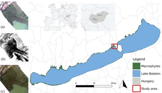
The study area is located at the Bozsai Bay on the northwest part of the Tihany Peninsula of Lake Balaton, Hungary (Figure 1) (Somlyody, Herodek, and Fischer 1983). It encom- passes a nature reserve of the Balaton Uplands National Park and as such is relative to
other reed beds of Lake Balaton, quasi-undisturbed from human activity. A variety of macrophytes, trees, and grasslands are encountered; however, reed is encountered frequently, especiallyPhragmites australis(Cav.) Trin. ex Steud, and to a smaller extent Typha angustifoliaL., Typha latifoliaL. andCarex sp.
In the last decades the stability of the waterward fringe of the reed bed has been deteriorating and the whole ecosystem has been retreating from the deep water, a phenomenon known as the‘reed dieback’(Van Der Putten1997; Stratoulias et al.2015).
As a consequence, the reed bed contains not only a diversity of vegetation species but also vegetation patches of different stability. The study area is situated in the vicinity of the Balaton Limnological Institute, providing easy access for fieldwork and assuring familiarity of the authors and experienced researchers with the local vegetation.
3. Airborne data
A European Facility for Airborne Research (EUFAR) airborne campaign was undertaken from 21 to 26 August 2010 by the NERC Airborne Research Facility by the UK Natural Environment Research Council (NERC). The platform used was a Dornier 228-101 research aircraft whichflew at 1550 m above mean sea level and was equipped with an Inertial Measuring Unit/Global Navigation Satellite System providing information on the aircrafts’position and orientation, respectively. The survey covered the whole lakeshore around Lake Balaton and the Kis Balaton, an adjacent wetland to the southwest of the lake. The data set comprised concurrently recorded hyperspectral imagery (400–2500 nm), discrete return lidar data, and orthophotos (Zlinszky et al.2011). In this study we use data from two adjacent flight strips (Figure 1) acquired on 21 August 2010 between 13:40 and 14:18 GMT (Table 1) over the Bozsai Bay which observes the Central European Summer Time.
Figure 1.Study area in the Bozsai Bay, Hungary (latitude 46.917899, longitude 17.835806). Inset numbered images depict thumbnails of the concurrently collected (a) hyperspectral image, (b) lidar data, and (c) orthophoto.
The hyperspectral data set was collected from an airplane-mounted Specim AISA dual system (Spectral Imaging Ltd., Oulu, Finland) integrating the nadir-looking sensors Eagle and Hawk as in similar studies (Artigas and Yang2005; Jensen et al.2007; Dalponte, Bruzzone, and Gianelle2008; Shafri and Hamdan,2009; Yang and Artigas2009; Burai et al.2010; Onojeghuo and Blackburn2011). The two sensors record incoming radiation cumulatively in 509 bands from 400 to 2450 nm with a spectral resolution (in full-width half-maximum (FWHM)) 2.20– 2.44 nm and 6.32 nm for Eagle and Hawk, respectively, and delivered a spatial resolution of 1.50 and 2.10 m, respectively (Table 1). The instruments are nadir-looking, and therefore, the angle between the line of sight of the sensors and the zenith is 180°.
Lidar data were recorded from a Leica ALS50 compact laser scanning system. A maximum of four discrete returns at 83 kHz (1064 nm) was delivered. At the last calibration before the 2010 campaign, lidar data were judged against ground control points and a mean error of 3.1 cm and standard deviation of 2.2 cm at an altitude of 1350 m was estimated.
True-colour orthophotos were recorded from a 39 megapixel Leica RCD105 medium format digital camera. The charge-coupled device instrument of the camera recorded radiation in three channels in the visible domain and delivered images in 16-bit TIFF format, with approximate ground resolution of 17.5 cm from 1550 m aircraft true altitude. Geometric registration on a projected coordinate system was implemented by the Technical University of Vienna. This data set was visually inspected synergistically with expert knowledge for selecting training and validation data sets from the hyperspectral images in the processes of classification and accuracy assessment, respectively. Further information on the airborne campaign and the sensors’specifications can be found at Zlinszky et al. (2012).
4. Methodology 4.1. Preprocessing
The hyperspectral and lidar data were preprocessed to derive meaningful information associated with lakeshore vegetation before the classification as illustrated inFigure 2.
Table 1.Specifications of remote-sensing instruments used to collect simultaneously hyperspectral imagery, lidar data, and orthophotos during 21–26 August 2010 around Lake Balaton, Hungary, under clear sky conditions.
Data type Hyperspectral Hyperspectral Discrete return lidar
Red, green, blue (RGB) photography
Instrument AISA Eagle AISA Hawk Leica ALS50-11 Leica RCD105
Ground pixel size (m) at 1550 m absolute altitude
1.50 2.10 4 returns maximum (resampled), 1 pt m−2stripwise point
density
0.175
Swathn (m) at 1550 m relative altitude (1445 m true altitude)
992 (38°field of view)
614 (24°field
of view) – 948
Spectral domain (nm) 400–970 970–2450 1064 Visible
Number of bands 253 256 Maximum four discrete returns 3
Band width (nm) 3.3 8.5 – RGB
Spectral resolution (FWHM) (nm) 2.20–2.44 6.31 – –
Radiometric resolution 12 bit 14 bit – 16 bit
Signal-to-noise ratio (SNR) 1250:1 (max) 800:1 (max) – –
The radiance values of the hyperspectral data were corrected for atmospheric effects, georeferenced, and mosaicked to compose a very fine spectral and spatial resolution image. A digital canopy model (DCM) was derived from the lidar data by subtracting the digital terrain model from the digital surface model (DSM), which are represented by the sensor’s last and thefirst return, respectively. Thereafter the DCM of the two adjacent stripes were mosaicked and resampled to 1.5 m pixel size with the nearest-neighbour interpolation method.
Focusing on the hyperspectral preprocessing, first a radiometric correction was applied to compensate for the effects of the off-nadir surface reflection and glint.
Vignetting effects, instrument scanning, off-nadir view angle, and sun reflection as well as other illumination effects can affect the image non-uniformly and are generally regarded as cross-track illumination effects (ITT Visual Information Solutions2009). In the used data set, the main contributor has been the sun reflection when solar position was diverging from the aircraft orientation (Table 2) and illumination conditions have there- fore not been isotropic. As a result, a glitter at the edge of the images is apparent in flights with north–south orientation. Moreover, the bands for Eagle were restricted to the bandwidth 450–900 nm and for Hawk to 1000–2400 nm as if the quality of the data degrades at the boundaries of the recording spectrum. Along-track mean values were then calculated and plotted to stress the variation in illumination differences across the Figure 2.Preprocessingflow chart of the hyperspectral and lidar data sets.
Table 2.Solar illumination conditions at Lake Balaton (latitude: 46.9127, longitude 17.8369) during time acquisition as calculated from the National Oceanic and Atmospheric Administration solar calculator (http://www.esrl.noaa.gov/gmd/grad/solcalc).
Flight number (Julian day) Date Time (GMT)* Solar noon Solar azimuth (°) Solar elevation (°)
233 21 August 2010 13:40–14:18 12:52 200.16–214.55 53:71–50:71
*Local time is + 1 h from the GMT and observes the Daylight Saving Time.
image lines. Cross-track illumination correction was applied on the samples of each image with a second-order polynomial function and an additive correction method.
Subsequently, atmospheric correction was implemented in the Fast Line-of-sight Atmospheric Analysis of Spectral Hypercubes (FLAASH), which is part of the Environment for Visualizing Images (ENVI) atmospheric correction module (ITT Visual Information Solutions 2009). FLAASH is afirst-principles atmospheric correction tool based on a modified version of the MODTRAN4 radiation transfer code (Matthew et al.2000) applicable in the visible through near-infrared and shortwave infrared regions up to 3μm. The FLAASH algorithm was selected (Supplemental material) based on the advantage of accounting for the adjacency effect, meaning the occurrence of optical path interference between reflectances from adjacent surface materials (Burazerovićet al.2013). This is especially prominent in coastlines, where existence of water and land, two materials with different spectral behaviour, is merging.
Moreover, the phenomenon is stronger at short wavelengths in scenes containing large reflectance contrast (Richter et al.2006), which is the case for the macrophytes growing in Lake Balaton, the water of which is characterized by high reflectivity in the optical domain due to the suspended sediment, submerged macrophytes, and high chlorophyll concentration of the lake water. Several studies have attempted to develop algorithms for correcting this phenomenon (i.e. Santer and Schmechtig2000; Sanders, Schott, and Raqueño2001; Sterckx, Knaeps, and Ruddick2011).
Considering the time period of the airborne campaign and the geographical position of the study area, the mid-latitude summer atmospheric model was used. No aerosol model was employed, as in the scene there was a lack of dark pixels, which is necessary for the implementation of aerosol integration (Kaufman et al.1997). Instead, the aerosol amount was estimated from the visibility which was set to 50 km in agreement with the atmospheric conditions on the day of the acquisition and confirmed by the local METAR report. The CO2
mixing ratio was set to 404 ppm. Spectral polishing was used with a width of nine spectral channels. The ground elevation at the lake is approximately 100 m above sea level and can be assumed constant for the purpose of atmospheric correction as the terrain around the lake is quiteflat. The rest of the input for FLAASH was taken from the navigationfile recorded during theflight campaign for each individual scene. Overall the atmospheric correction provided typical spectral responses for the vegetation contained in the image (Supplemental material).
No artefacts were apparent due to the clear sky conditions at the time of image acquisition and the lack of absorbing bodies that qualify as‘open water’in the spectral sense around the mesotrophic and sediment-laden Bozsai Bay.
Last, geometric registration was applied with the open-source Airborne Processing Library (APL) software v3.1.4 (Warren et al.2014). The algorithm is designed to geocode the raw imagery by taking into account bore-sight information recorded during theflight. The DSM extracted from the concurrently acquired lidar data set with missing valuesfilled-in from the Advanced Spaceborne Thermal Emission and Reflection Radiometer Global DEM (NASA LP DAAC2001) was used to increase the geometric precision. The mean absolute along-track and across-track error (at nadir and measured in pixel size) reported from APL developers is 0.39 ± 0.31 and 0.65 ± 0.42, respectively (Warren et al.2014), which translates for the data set used in this study to 0.58 ± 0.46 m (along track) and 0.97 ± 0.63 m (across track) for Eagle and 0.82 ± 0.65 m (along track) and 1.36 ± 0.88 m (across track) for Hawk. The two adjacent hyperspectral images were registered at the UTM projected coordinate system (Zone 33N) of the World Geodetic System 1984 Datum on a 1.5 m × 1.5 m grid (Figure 3).
4.2. Training and validation sets
Chen and Stow (2002) made a thorough comparison of common training strategies for classification methods used in the literature and reckon that the training approach can affect the classification result. Moreover, they claim that the training has a higher influence on the result when applied on fine rather than coarse resolution images.
Information on vegetation species and geolocation of pure areas formed the basis for selecting the training and validation data sets. For the reed-specific vegetation types, ecologists who are familiar with the study area advised on the definition of the classes. A set of polygons was selected from the hyperspectral image representing the seven emergent-vegetation classes of interest and was verified for homogeneity and repre- sentation with the orthophotos. A stratified random sampling (probabilistic method of sampling) was followed for the reason of minimising variability within different zones of the image. The sampling area was divided in large zones and each one was assigned a number of sample units. The position of the units then was defined randomly and the size of the samples was proportional to the size of the class they represent. The concurrently acquired aerial photography was used to assure coherency of the poly- gons. The set was divided into two groups; thefirst group comprising 18 polygons (total area 147,228 m2) was used for training the classifier and the second group comprising 16 polygons (total area 92,920 m2) for validating the results (Figure 3).
4.3. Input layers
The input layers for the classification process were prepared from the Eagle, Hawk, and lidar data (Figure 4). Thefirst input layer was extracted from the Eagle data set while the Figure 3.Near IR composite (RGB: 700, 545, and 341 nm) of the hyperspectral Eagle post-processed image and the training and validation polygons used for thefirst classification of the image in the main vegetation classes.
second input layer was created in a similar manner from the Hawk data. The third image input for the classification is a layer stack including vegetation indices demonstrating the highest degree of association with reed stability and photosynthetic performance in Lake Balaton as studied by Stratoulias et al. (2015) and popular empirical narrowband indices. These are respectively three reflectance ratios associating to Fs, Fm, and PAR, the photochemical reflectance index (PRI), the normalized difference vegetation index (NDVI), and thefirst three principal components (PCs) (Figure 4). Finally, the last input layer is based on the three PCs of the Eagle image and the DCM extracted from the lidar data. Two adjacent hyperspectral scenes were used which comprise the reed bed and neighbouring grasslands, agriculturalfields (rape, barley, and wheat), roads, settlements, and trees.
The first input layer is solely based on the visible spectrum provided by the Eagle data. Due to the nature of hyperspectral data, the spectral bands are highly correlated and the data set in whole contains a large degree of redundancy. A minimum noise fraction (MNF) transformation (Green et al.1988) can be applied to eliminate the noise, reduce the dimensionality of the data, and hence the computational requirements without important loss of information. Subsequently, the components (i.e. eigenvalues) of the transformation which are unaffected from noise can be inversed back to the real hyperspace. Pandey, Tate, and Balzter (2014) found that the classification accuracy Figure 4.Workflow indicating the preparation of input layers for the classification process based on the Eagle, Hawk, and lidar preprocessed data sets.
improves in case ML algorithm is applied on the MNF eigenvalues instead of the total number of bands.
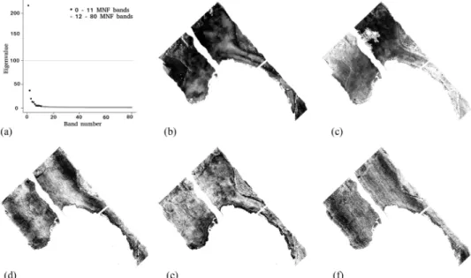
Forward MNF transformation was applied on the Eagle image. Based on the eigen- values and the corresponding MNF bands, thefirst 14 transformed bands were selected as the threshold where information is still more prominent in the image in comparison to noise (Figure 5).
The Hawk data are paying in the near-infrared domain and have been acquired simultaneously with the Eagle data; nevertheless, the coverage of the whole reed bed is not complete due to its narrower swath, and adjacent images do not overlap. This appears as a wide missing stripe at the edge of the individual images. Furthermore, Hawk suffers from regular dropped frames, resulting in missing lines in the image. The integration of the Hawk data in the methodology was attempted to evaluate the usefulness of the infrared spectral domain in wetland vegetation mapping. A similar methodology as for Eagle data was followed. Bands between 1336–1462 nm and 1791– 1967 nm have been excluded as they are largely affected by atmospheric water vapour absorption. The MNF was then calculated and the first 11 eigenvalues selected in a similar procedure as described in the previous part (Figure 6).
The third data set was based on the assumption that complementary data from lidar and hyperspectral sensors can provide a robust information set. Despite the fact that the DCM derived from moderate-density lidar data underestimates the canopy height (Zlinszky et al. 2012), it is however associated to the canopy height characteristics. The first three PCs from the Eagle image were extracted and combined with the DCM to enhance the information content. The last data set is based on narrowband empirical indices which are associated with reed physiolo- gical stability at the specific area of study. Thefirst three PCs from the Eagle image
Figure 5.Eigenvalues of the Eagle image (a) and depictions of the minimum noise fraction (MNF) transformation corresponding to band numbers 1 (b), 4 (c), 9 (d), 14 (e), and 16 (f). Noise is considerably higher than the information content after band 14 and hence all the bands after this threshold have been dropped.
were calculated. The narrowband empirical indices NDVI (Tucker 1979) and PRI (Gamon, Penuelas, and Field 1992) were extracted. These are indices heavily used in vegetation-related studies as they are associated to vegetation characteristics.
Furthermore, the band rations representing the Fs, Fm´, and PAR per findings of the fluorescence analysis of macrophytes in Lake Balaton as suggested by Stratoulias et al. (2015) were used. The individual layers were combined in a composite image.
4.4. Reed bed masking and mosaicking
The interest of this study lay in the reed bed of the Bozsai Bay. The macrophytes encountered in this nature reserve inherit a diverse and complex structure, and it was decided to narrow the focus on the emergent macrophytes of this area rather than a broader categorization of vegetation types on the lakeshore. Trees, lake water, bare ground, and man-made materials, some of which are within the nature reserve, were excluded.
A mask from the DCM was derived by selecting all pixels with values between 0.3 and 3 m, range which represents typical macrophytic vegetation. The hyper- spectral image was subset with the mask to isolate pixels of macrophytes. Finally, a mosaicking procedure was undertaken to stitch together the two images. No colour balancing was used and a feathering distance of 100 pixels was assumed.
Figure 6.Eigenvalues of the Hawk image (a) and depictions of the minimum noise fraction (MNF) transformation corresponding to band numbers 1 (b), 4 (c), 9 (d), 11 (e), and 12 (f). Noise is considerably higher than the information content after band 11 and hence all the bands after this threshold have been dropped.
4.5. Classification
Several processing steps were iteratively tested and led to the consolidated methodo- logical workflow presented in Figure 7. The classification procedure was conducted identically for the four different input layers developed and using the same training data set. The image was first classified based on the dominant macrophytes encoun- tered in the area. These classes werePhragmites, Typha, Carex,and grassland (this latter constituted by herbaceous (non-woody)) vegetation managed by summer mowing at least once a year. ThePhragmitesclass was used to subset the original input layer again, and this subset image was then classified based on the dominance ofPhragmitesin the patch according to the classes of dominant, co-dominant, subdominant, and reed die- back. Reed dominant is the category in whichPhragmitesrepresents at least 80% of the plant cover density as observed duringfieldwork. Reed co-dominant is the category with at least 50% of Phragmites. When other macrophytes such as Typha and Carex are dominant and there is a minor coverage of Phragmites, then this defines the
Figure 7.Workflow of the classification scheme developed through iterative classifications and evaluations for mapping emergent vegetation. The two-step approach involves classification of the image based on the main macrophyte species (Phragmites, Typha, Carex, and grassland) and subsequently isolation of thePhragmites class and classification of the latter based on the dom- inance of Phragmites (dominant, co-dominant, and subdominant) and reed dieback. At the final stage, the two classification results are merged with the Phragmites-specific classification overlaid over the macrophyte species map. The result is assessed quantitatively based on expert knowledge and concurrently acquired orthophotos.
subdominant category. Finally, reed dieback is the area where reed degraded naturally and is typically encountered at the waterfront edge of the reed bed, where only Phragmitesis present.
Subsequently, the two classification products were merged with the subclasses of Phragmites substituting the generic class Phragmites in the main classification. This scheme was applied twice, first based on the ML algorithm and a second time based on SVM for each input layer. Image processing and classification were realized with the software ENVI 5.0. The cartographic production was carried out in ArcMAP 10.0 (Environmental Systems Research Institute, Inc.).
4.6. Accuracy assessment
Classification of remote-sensing data has no credibility unless its accuracy is assessed (Chen et al. 2004). The methodology for accuracy assessment using an error matrix (contingency table) was followed (Congalton 1991). An approach presented by Dalponte, Bruzzone, and Gianelle (2008) in a study employing similar data has been adapted. As already mentioned, in situ floristic information synergistically with the concurrently acquired high-resolution orthophotos and expert knowledge were com- bined to create the validation polygons. The validation polygons were overlaid on the high-resolution orthophotos and were used together with expert knowledge to decide on the vegetation class representation. Given the homogeneity of the poly- gon, which was taken into account when designing the sample polygons, the ascribed classes were considered the ground truth data. The accuracy assessment was carried out by comparing the thematic map with the validation data using a confusion matrix.
5. Results
Figures 8 and 9 present the results of the classification based on ML and SVM algo- rithms, respectively, and for each data source.Tables 3and4present the error matrix of the accuracy assessment for each classification algorithm independently. The maps contain solely classes of emergent macrophytes typically encountered around Lake Balaton. The overall accuracy ranges from 41.79% for the lidar data set with ML classification to 88.64% for the Eagle data set with SVM.
Reed in the central part of the reed bed was classified as co-dominant and botanical surveys support thisfinding, while at the edges (both terrestrial and waterward) of the reed bed and especially in the thin sliver at the west reed bed seems to compete with other macrophyte species. The main class (i.e. Phragmites) typically grows in the same environment with other macrophyte species and grasses, and hence the dominant class in all classification results is reed co-dominant which occupies the main reed bed.
Co-dominant reed is very accurately classified by SVM in the cases of Eagle and indices layers with 96% and 97% producer accuracy. Pure reed (i.e. reed dominant) is encountered at a small part of the Lake shore east of the Typha island, part which is correctly classified with both ML and SVM in all data sources except lidar; in the case of SVM this part is only slightly containing reed dominant pixels while with ML a large part of the image is classified as reed dominant which is incorrect.
The canopy structure information contained in the lidar does not assist in the classification of this class. SVM shows a higher accuracy for Eagle and indices data sources (84% and 68%, respectively) in comparison to ML; however, when classifying Hawk data ML has an advantage of producer accuracy 60% over 40% for SVM.
It is worth noting that reed dominant has the lowest accuracy across macrophytes as homogeneous and pure patches of Phragmites are not frequently encountered in the Bozsai Bay and to an extent they always contain a degree of other macrophyte species within a pixel. Reed subdominant contains reed as a minority within other macrophytes, Figure 8.Thematic maps from the ML classification of the Eagle (a), Hawk (b), indices from Eagle (c), and lidar combined with Eagle PCs (d) of the macrophyte main species andPhragmitesassociations at Bozsai Bay, Lake Balaton.
and is encountered at the edge of the reed bed, where terrestrial vegetation and grass grow in favourable conditions. ML and SVM are classifying the east part of the reed bed as reed subdominant as well as fringe areas of the reed bed. One important difference is found on the north part of the reed bed where there is a sliver of grassland as indicated by SVM classifications of Eagle image and the indices image; however, ML classifies this part mainly as reed subdominant which is incorrect. ML always provides better producer accuracy than SVM, while the opposite is realized for the case of user accuracy; in Figure 9.Thematic maps from the SVM classification of the Eagle (a), Hawk (b), indices from Eagle (c), and lidar combined with Eagle PCs (d) of the macrophyte main species and Phragmites associations at Bozsai Bay, Lake Balaton.
Table3.ConfusionmatrixillustratingtheresultsoftheclassificationofthefourinputscenarioswiththeMaximumLikelihood(ML)algorithm. TyphaGrasslandCarexReeddominant EagleHawkIndicesLidarfusionEagleHawkIndicesLidarfusionEagleHawkIndicesLidarfusionEagleHawkIndicesLidarfusion Typha95635741–3–1–29–0602317 Grassland––––25–76–––––––– Carex––––––––95–8173–––– Reeddominant–4733––10–––065605563 Reedco-dominant–29302346311381317014513 Reedsub-dominant14–56950849243368241381 Reeddieback4–6192–5––––131274 Produceraccuracy9563574125–7695–817365605563 Overallaccuracy(%)83.2264.4469.0541.79 Kappacoefficient0.720.450.520.26 Reedco-dominantReedsubdominantReeddiebackUseraccuracy EagleHawkIndicesLidarfusionEagleHawkIndicesLidarfusionEagleHawkIndicesLidarfusionEagleHawkIndicesLidarfusion Typha00101100231–328144129 Grassland––––––––––––100–100100 Carex0–443–01––––82–5754 Reeddominant622238001317–9234315339 Reedco-dominant866374314285–51–98879388 Reedsubdominant715913899470652620312971636356 Reeddieback1––321576841586049433218 Produceraccuracy866374318994706568415860 Allvaluesexceptthekappacoefficientareinpercentages.
Table4.ConfusionmatrixillustratingtheresultsoftheclassificationofthefourinputscenarioswiththeSupportVectorMachines(SVM)algorithm. TyphaGrasslandCarexReeddominant EagleHawkIndicesLidarfusionEagleHawkIndicesLidarfusionEagleHawkIndicesLidarfusionEagleHawkIndicesLidarfusion Typha5459208–0––––––10101 Grassland–15––92696839–––––3–– Carex––––––––8430–––0–– Reeddominant194970–1–––––84406851 Reedco-dominant10206880126941457979511421844 Reedsubdominant21–0651857112350801 Reeddieback15135––30––––2521 Produceraccuracy5459208926968398430––84406851 Overallaccuracy(%)88.6479.4977.6968.72 Kappacoefficient0.800.650.590.43 Reedco-dominantReedsubdominantReeddiebackUseraccuracy EagleHawkIndicesLidarfusionEagleHawkIndicesLidarfusionEagleHawkIndicesLidarfusionEagleHawkIndicesLidarfusion Typha00101012523675792614 Grassland000–0100144097799796 Carex00––04––––––9456–– Reeddominant28010212073267665233420 Reedco-dominant968597871432135111492898376 Reedsubdominant261275865450138372892828473 Reeddieback––0062237234434937464545 Produceraccuracy968597877586545072344349 Allvaluesexceptthekappacoefficientareinpercentages.
essence this means that SVM results show a realistic map of subdominant reed; how- ever, several pixels from the validation set have not been labelled correctly by SVM and therefore some pixels of this class are misclassified as other classes on this map.
Reed dieback is encountered at the waterward edge of the northeast part of the reed bed mainly as fragmented patches of water reed. Reed dieback is confused mainly with reed subdominant and to a lesser extent withTypha as it is mainly neighbouring with thefirst and the fringe of theTyphaisland is misclassified as dieback in several cases in regard to the latter. This also means that spectrally, and at 1.5 m spatial resolution, dieback is different than the more homogeneous classes of dominant and co-dominant reed. SVM overestimates the extent of reed dieback in the case of Eagle data in comparison to the ML results, while the opposite is the case for the indices composite image. An ML classification of the lidar data presents unrealistic results while the SVM is able to indicate the extent of the dieback reed.
Studies in the literature are controversial about the capability of imaging spectro- scopy for mapping vegetation stress. Swatantran et al. (2011), for example, mentioned that hyperspectral data can provide information such as stress on canopy state, while Leckie et al. (2005) attempted unsuccessfully to include unhealthy classes of species in a classification of old growth temperate conifer forest canopies. Zlinszky et al. (2012), using only airborne lidar-based radiometry and structure metrics, reported accuracies of 62% and 76% specifically for reed dieback.
In this study, representative polygons of reed dieback areas were selected; however, reed dieback is a dynamic phenomenon characterizing the physiological condition of a plant and not a vegetation category with concrete boundaries. As such reed dieback areas are indicated by the fragmentation of the reed patch rather than the physiological status of the plant in this classification scheme–this is why lidar proved successful in recognizing the characteristic fragmentation. For a more representative estimation of the physiological status, spectral indices can show the degree to which the area is stable (Stratoulias et al. 2017). However, integrating the dieback class in a macrophyte classi- fication scheme provides an indication of fragmented and sparse reed patches which are under unfavourable environments at the period of image acquisition and hence poten- tially associated with reed dieback conditions.
Typha, occupying the small island in the centre of the image, is correctly classified in all ML results; however, in the cases of the indices and lidar layers severalTyphapatches are indicated in the reed bed erroneously as indicated by the relatively higher user’s accuracy error in these two data sources (Table 3). In the case of the SVM algorithm (Table 4), the Eagle classification provides similar results to the ML results, and the indices and lidar layers indicate the outer buffer zone as reed co-dominant. Typha is often confused with other assemblages ofPhragmites, a fact which is also reported in a similar study from Maheu-Giroux and De Blois (2005) using colour aerial photography and by Zlinszky et al. (2014) using lidar. Carex is encountered at the west of the reed bed, classified correctly only in the case of Eagle data for both algorithms with 82% and 94% user accuracy, respectively; however when using the Hawk data, ML does not classify any pixel asCarex and instead replaces it withTypha. SVM, on the other hand, presents an area restricted in size. In the case of indices and lidar, there is a fragmented distribution in other parts of the image as well as for the ML classification, while SVM
does not classify Carex pixels. Again the most representative source for pure macro- phytes species is the Eagle instrument.
Grassland is a class differing in foliage height from all the other vegetation types of the study area and hence it would be expected to be distinguished from the lidar composite image; however, this is not the case for ML (producers’ accuracy 6%); SVM only partially classifies the sliver on the north part of the image (producers’ accuracy 39%). ML in all cases does not perform satisfactorily in the case of grassland as it is most often classified as reed subdominant. This is because the transition from the reed bed to the grassland does not have a crisp boundary but occurs gradually in a buffer zone where the two species coexist in different proportions. SVM applied on the Eagle data set is outperforming considerably for the grass class with 92% producer accuracy and 97% user accuracy.
Regarding the comparison of the two classifiers, overall SVM provides more accurate results than ML, a fact also observed in a similar study mapping submerged macro- phytes by Hunter et al. (2010). However, some errors exist between the different classes of reed and especially the classes encountered at the edge of the reed bed, for instance, reed dieback and sub-dominant reed. Moreover, we observe that ML is not performing well when classifying multisource images while SVM is not confused by this approach.
ML seems to underperform when classifying data sets comprising different data types, such as the lidar or the Hawk integrated with the Eagle data. Overall, our study is in agreement with Pal and Mather (2005), who argued that SVM achieves higher level of classification accuracy. This fact can be attributed to two reasons for the case of mapping aquatic vegetation;first, thefine resolution required to map the small extent of a typical aquatic vegetation patch restricts the number, and most importantly the size, of the training data sets to be used in the classification training; second, the hyperspectral data, required to discriminate the complex vegetation status of these types of ecosystems, is introducing high dimensionality in the input data source. Both constrains have proven to be an advantage of the SVM classifier over ML.
While satellite hyperspectral systems are still limited, very fine spatial resolution satellite imagery has been lately available raising similar classification challenges as addressed in this study. Mapping small-scale phenomena, such as lakeshore vegetation, requires a different approach than the application of traditional classifiers (e.g. ML) on traditionally medium-resolution data sets (e.g. Landsat) and therefore the approach to the problem needs to be refined. In this study, we suggest that forfine-scale vegetation mapping the spectral information in the visible and near-infrared provides the most discriminatory power in comparison to longer wavelengths, lidar or the fusion of these data sets. The SVM classifiers are suggested for small-scale phenomena for compensat- ing for the limitation of small training sampling. Potentially, other classification approaches, such as fuzzy classification and machine learning techniques, could provide robust results on different levels of vegetation class mixing encountered in the study area.
6. Conclusions
Classification results derived from ML and SVM classifiers with four different airborne input data sources have been presented. Hyperspectral Eagle and Hawk data have been
used independently and synergistically with lidar data to map emergent macrophytes in a nature reserve on the shore of Lake Balaton. A detailed representation of most classes was achieved, which can be attributed to the concurrent very high spectral and spatial resolution of the imagery.
Significant preprocessing is required for the airborne hyperspectral data before the classification. While classification techniques can be automated given the availability of a training dataset, preprocessing is site- and image-specific and the intervention of the user is essential. Field data are an important part of mapping aquatic vegetation; a classification based solely on the airborne imagery and without the contribution of information on the ecological status of the training samples would not provide ecolo- gically meaningful results.
Phragmitesis growing in the same environment as other macrophytes and grasses, especially in the terrestrial part of the reed bed. Hence, there is an abundance of reed within any single pixel. In this study, a categorical approach of reed abundance and other macrophyte species as well as grasses was chosen. The reed subclasses show a high degree of separability, with the most prominent class (co-dominant reed) exhibit- ing 96% producers’accuracy and 92% users’accuracy when an SVM is applied to Eagle data. Reed dieback is the most challenging case of vegetation mapping and unique since it refers to a state of deterioration of the vegetation species rather than species or association of species. Nevertheless, fragmentation at the edge of the reed bed is associated to the consequences of the dieback conditions and hence the extent to which the reed bed is affected.
In agreement with other studies, SVM outperforms ML, mainly for the grassland class, and provides higher overall accuracy with any of the data sources, reaching 89% for optical input data together with near-infrared data. The joint classification of a simple lidar-based canopy model with thefirst three PCs from the Eagle image did not perform satisfactorily (overall accuracy 69%,κ= 0.43), which might be attributed to the fact that different macrophytes have a similar canopy structure to be distinguished from a lidar- derived CHM fromfirst and last returns, unlike the high contrast the CHM indicated for more generic classes. However, additional lidar texture indicators such as sigma(z), height variance, or height ranges in a neighbourhood might provide more powerful indicators of vegetation structure (beyond height). Macrophyte associations and species encountered in a typical reed bed on the shore of Lake Balaton are identified using the MNF transformation of high spatial resolution hyperspectral data, especially in the visible and near-infrared spectrum.
The main conclusion of this study is that the classification of solely hyperspectral visible and near-infrared data between 400 and 1000 nm provides the most accurate results in contrast with synergistic classification of hyperspectral data and a CHM or even hyperspectral data extending up to 2500 nm. Moreover, in the case of classification of aquatic resolution at a fine spatial and spectral scale the SVM classifier has overall provided more accurate results in comparison to ML.
Acknowledgments
This work was supported by GIONET, funded by the European Commission, Marie Curie Programme, Initial Training Networks under Grant Agreement PITN-GA-2010-26450. The airborne
data were collected and provided by the Airborne Research and Survey Facility vested in the Natural Environment Research Council under the EUFAR Contract Number 2271. AZ was sup- ported by the Hungarian Scientific Research Fund OTKA grant PD 115833. H. Balzter was supported by the Royal Society Wolfson Research Merit Award, 2011/R3 and the NERC National Centre for Earth Observation.
Disclosure statement
No potential conflict of interest was reported by the authors.
Funding
This work was supported by GIONET, funded by the European Commission, Marie Curie Programme, Initial Training Networks under [Grant Agreement PITN-GA-2010-26450]. The airborne data were collected and provided by the Airborne Research and Survey Facility vested in the Natural Environment Research Council under the [EUFAR Contract Number 2271]. AZ was sup- ported by the Hungarian Scientific Research Fund OTKA [grant PD 115833]. H. Balzter was supported by the Royal Society Wolfson Research Merit Award, 2011/R3 and the NERC National Centre for Earth Observation.
ORCID
Dimitris Stratoulias http://orcid.org/0000-0002-3133-9432
References
Adam, E., O. Mutanga, and D. Rugege.2010.“Multispectral and Hyperspectral Remote Sensing for Identification and Mapping of Wetland Vegetation: A Review.” Wetland Ecology and Management18 (3): 281–296. doi:10.1007/s11273-009-9169-z.
Anderson, K., J. Bennie, and A. Wetherelt. 2010.“Laser Scanning of Fine Scale Pattern along a Hydrological Gradient in a Peatland Ecosystem.”Landscape Ecology25: 477–492. doi:10.1007/
s10980-009-9408-y.
Artigas, F. J., and J. S. Yang. 2005.“Hyperspectral Remote Sensing of Marsh Species and Plant Vigour Gradient in the New Jersey Meadowlands.”International Journal of Remote Sensing26 (23): 5209–5220. doi:10.1080/01431160500218952.
Bahria, S., N. Essoussi, and M. Limam.2011.“Hyperspectral Data Classification Using Geostatistics and Support Vector Machines.” Remote Sensing Letters 2: 99–106. doi:10.1080/
01431161.2010.497782.
Baker, C., R. Lawrence, C. Montagne, and D. Patten.2006.“Mapping Wetlands and Riparian Areas Using Landsat ETM+ Imagery and Decision-Tree-Based Models.” Wetlands 26 (2): 465–474.
doi:10.1672/0277-5212(2006)26[465:MWARAU]2.0.CO;2.
Balzter, H., A. Luckman, L. Skinner, C. Rowland, and T. Dawson.2007.“Observations of Forest Stand Top Height and Mean Height from Interferometric SAR and Lidar over a Conifer Plantation at Thetford Forest, UK.”International Journal of Remote Sensing 28 (6): 1173–1197. doi:10.1080/
01431160600904998.
Bartlett, D. S., and V. Klemas. 1980.“Quantitative Assessment of Tidal Wetlands Using Remote Sensing.”Environmental Management4 (4): 337–345. doi:10.1007/BF01869426.
Boyd, D., C. Sanchez-Hernandez, and G. Foody.2006.“Mapping a Specific Class for Priority Habitats Monitoring from Satellite Sensor Data.”International Journal of Remote Sensing27 (13): 2631– 2644. doi:10.1080/01431160600554348.