33(2006) pp. 125–140
http://www.ektf.hu/tanszek/matematika/ami
Performance modeling tools with applications ∗
János Sztrik
a, Che Soong Kim
baFaculty of Informatics, University of Debrecen e-mail: jsztrik@inf.unideb.hu
bDepartment of Industrial Engineering, Sangji University e-mail: dowoo@mail.sangji.ac.kr
Submitted 10 March 2006; Accepted 1 October 2006
Abstract
This paper deals with the role of performance modeling tools. It intro- duces 3 major tool development centers and shows how a given tool can be applied to investigate the performance of a finite-source retrial queueing sys- tem.
Keywords: Performance tools, tool support, finite-source retrial queueing sys- tems.
1. Introduction
The argument for performance engineering methods and tools to be employed in computer-communication systems has always been that such systems cannot be designed or modified efficiently without recourse to some form of predictive model, just as in other fields of engineering. This argument has never been more valid than it is with today’s highly complex combination of communication and com- puter technologies. These have created the Internet, the Grid and diverse types of parallel and distributed computer systems. To be practical, performance engineer- ing relies on tools to render its use accessible to the non-performance specialist, and in turn these depend on sound techniques that include analytical methods, sto- chastic models and simulation. Tools and techniques also need to be parameterised and validated against real world observations, requiring sophisticated measurement
∗Research is partially supported by KOSEF-Hungarian Academy of Sciences Bilateral Scientific Cooperation Grant KOSEF F01-2006-000-10014-0, 2004 and Hungarian Scientific Research Fund- OTKA K60698/2005
125
techniques in this picosecond cyber-world. The series of "International Confer- ences on Modelling Techniques and Tools for Computer Performance Evaluation"
(TOOLS) has provided a forum for this community of performance engineers with all their diverse interests and selected papers of these conferences have been pub- lished in the reputed Performance Evaluation journal. Many mathematical techniques have been developed to derive various measures from Markov reward models which form the basis of almost all performability models. For evaluation techniques to be used, software tools are needed. The interested reader is referred to, among others, [8, 7] for comprehensive and very detailed surveys on relevant tools.
The paper is organized as follows. Section 2 is devoted to the introduction of some recent well-known tools. In Section 3 tool supported analysis of finite-source retrial queueing systems with a server subject to breakdowns is performed. Finally, some conclusions are made.
2. Some recent modeling tools
In the following 3 major tool development centers are introduced.
2.1. Tools at Faculty of Informatics, University of Dortmund, Germany
This traditionally famous center has developed several software packages which can be downloaded from the site:
http://ls4-www.informatik.uni-dortmund.de/tools.html
Parallel to their methodological work the center continuously developed and used tools for performance evaluation. Their intention is to provide facilities for a model description close to the original system specification and hiding details of the analysis techniques. Such tools map the model specification automatically to an analysable model. The set of tools developed by Informatik IV comprises amongst others
• HIT: The software tool HIT provides for model-based performance evalu- ation of computing and communication systems during all phases of their life cycle. Specification of (models of) dynamic, discrete-event, stochastic systems is achieved by particular language- and graphics-based description options. Performance evaluation of accordingly specified models is supported by a variety of techniques of the simulative and analytical types.
• HiQPN:HiQPN-Tool supporting the analysis of hierarchical QPN models, a superset of Coloured GSPNs and Queueing Networks. These models can be analysed with respect to qualitative and quantitative aspects.
• DSPNexpress: DSPNexpress is a software package for performance and reliability modelling of computer systems with deterministic and stochastic Petri nets (DSPN). DSPNexpress has a user-friendly graphical interface for definition, analysis and graphical animation of DSPNs. The package has been called DSPNexpress because this software package solves complex DSPNs with four orders of magnitude less CPU time than other packages previously introduced.
• APNN-Toolbox: The APNN-Toolbox is a software package for functional (invariant, liveness, model checking) and quantitative analysis (APNNsim, NSolve, Parallel, SupGSPN) of GSPNs. Modeling of GSPNs can be realized with the editor APNNed. The editor can start the analysis tools and after- wards a visualization of the results is possible. The communication between APNNed and the analyzers takes place by a common exchange interface so- called Abstract Petri net notation (APNN).
All tools provide a graphical user interface and are available for usual type of work- stations. They are tested exhaustively and have been employed for the evaluation of operating systems in the development phase, future hardware architectures, and the assessment of distributed and telecommunication systems. The tools also suit for an evaluation of flexible manufacturing systems. Their practical usability has been proved by a large number of external installations in universities, research institutes and industry.
2.2. Möbius Tool
Möbius is a software tool for modeling the behavior of complex systems, see [5]. It is one of the major research projects of the Performability Engineering Research Group (PERFORM) in the Coordinated Science Laboratory at the Uni- versity of Illinois at Urbana-Champaign, USA. Although it was originally developed for studying the reliability, availability, and performance of computer and network systems, its use has expanded rapidly. It is now used for a broad range of discrete- event systems, from biochemical reactions within genes to the effects of malicious attackers on secure computer systems, in addition to the original applications. That broad range of use is possible because of the flexibility and power found in Möbius, which come from its support of multiple high-level modeling formalisms and multi- ple solution techniques. This flexibility allows engineers and scientists to represent their systems in modeling languages appropriate to their problem domains, and then accurately and efficiently solve the systems using the solution techniques best suited to the systems’ size and complexity. Time- and space-efficient discrete-event simulation and numerical solution are both supported. Features of the tool is the following.
• Multiple modeling languages, based on either graphical or textual representations: Supported model types include stochastic extensions to Petri nets, Markov chains and extensions, and stochastic process algebras.
Models are constructed with the right level of detail, and customized to the specific behavior of the system of interest.
• Hierarchical modeling paradigm: Build models from the ground up.
First specify the behavior of individual components, and then combine the components to create a model of the complete system. It is easy to combine components in multiple ways to examine alternative system designs.
• Customized measures of system properties: Construct detailed ex- pressions that measure the exact information desired about the system (e.g., reliability, availability, performance, and security). Measurements can be conducted at specific time points, over periods of time, or when the system reaches steady state.
• Study the behavior of the system under a variety of operating con- ditions: Functionality of the system can be defined as model input parame- ters, and then the behavior of the system can be automatically studied across wide ranges of input parameter values to determine safe operating ranges, to determine important system constraints, and to study system behaviors that could be difficult to measure experimentally with prototypes.
• Distributed discrete-event simulation: Evaluates the custom measures using efficient simulation algorithms to repeatedly execute the system, either on the local machine or in a distributed fashion across a cluster of machines, and gather statistical results of the measures.
• Numerical solution techniques: Exact solutions can be calculated for many classes of models, and advances in state-space computation and gen- eration techniques make it possible to solve models with tens of millions of states. Previously, such models could be solved only by simulation.
The Möbius tool was built based on the belief that no one modeling formalism can be the best way to build all models of systems from across the diverse spectrum of application domains. In addition to the fact that many domain-specific modeling languages are needed, we also need many techniques (for example, simulation, state space exploration, and analytical solution) for analyzing models to study important behaviors of the systems being modeled. Möbius addresses those issues by defining a broad framework in which new modeling formalisms and model solution methods can be easily integrated, and populating that framework with multiple, synergisti- cally combined modeling formalisms and model solution methods. Many advanced modeling formalisms and innovative and powerful solution techniques have been integrated in the Möbius framework. It is available for the following operating systems: Windows XP or 2000, and Linux Fedora Core 3 and later. The package can be found athttp://www.mobius.uiuc.edu/
2.3. MOSEL Tool
Performance modeling tools usually have their own textual or graphical specifi- cation language which depends largely on the underlying modeling formalism. The different syntax of the tool-specific modeling languages implies that once a tool has been chosen it will be difficult to switch to another one as the model has to be rewritten using a different syntax. On the other hand the solution of the underly- ing stochastic process is performed in most tools by the same standard numerical algorithms. Starting from these observations the creation of MOSEL (MOdeling, Specification and Evaluation Language) tool, developed at the University of Er- langen, Germany, is based on the following idea: Instead of creating another tool with all the components needed for system description, state space generation, sto- chastic process derivation, and numerical solution, we focus on the formal system description part and exploit the power of various existing and well tested packages for the subsequent stages. MOSEL is a modeling environment which comprises a high-level modeling language that provides a very simple way for system descrip- tion. In order to reuse existing tools for the system analysis, the environment is equipped with a set of translators which transform the MOSEL model specification into various tool-specific system descriptions [3].
The main features of the MOSEL-environment are the following:
• The modeler inspects the real-world system and generates a high-level system description using the MOSEL specification language. He also specifies the desired performance and reliability measures using the syntax provided by MOSEL. He passes the model to the environment which then performs all following steps without user interaction.
• The MOSEL environment automatically translates the MOSEL model into a tool-specific system description, for example a CSPL-file suitable to serve as input for SPNP.
• The appropriate tool (i.e. SPNP) is invoked by the MOSEL-environment.
• The state space of the model is generated by the tool according to the se- mantic rules of its modeling formalism out of the static model description.
• The semantic model is mapped onto a stochastic process.
• The stochastic process is solved by one of the standard numerical solution algorithms which are part of the tool. The results of the numerical analysis are saved in a file with a tool-specific structure.
• The MOSEL-environment parses the tool-specific output and generates a result file (sys.res) containing the performance and reliability measures which the user specified in the MOSEL system description. If the modeler requested graphical representation of the results, a second file (sys.igl) is generated by MOSEL [3, 4].
The latest version of MOSEL, called MOSEL-2 has been developed by Jörg Barner and Björn Beutel, see [2]. Moreover, the present version contains the enhanced MOSEL to CSPL translator written by Patrick Wüchner, see [9]. The distribution contains the MOSEL source code (written in C) as well as a collection of examples and installation instructions. Moreover, Björn’s diploma-thesis is included in PDF- format. Chapter 4 of his thesis contains an easy-to-read introduction to modeling and performance evaluation with MOSEL-2. MOSEL-2 provides means by which many interesting performance or reliability measures and the graphical presentation of them can be specified straightforwardly. It is especially easy to evaluate a model with different sets of system parameters. The benefit of MOSEL-2 - especially for the practitioner from the industry - lies in its modelling environment: A MOSEL-2 model is automatically translated into various tool-specific system descriptions and then analyzed or simulated by the appropriate tools. This exempts the modeler from the time-consuming task of learning different modeling languages. MOSEL is available under the GNU Public License (GPL). You might read the installation instructions first. All information concerning the package can be found at web address http://www4.informatik.uni-erlangen.de/Projects/MOSEL/
System requirements:
• MOSEL-2 should be easily portable to nearly every POSIX system on which an ISO C90 compiler is running.
• You may compile MOSEL-2 using the Portable GNU C Compiler GCC, avail- able fromhttp://www.gnu.org.
• It has already been tested under the Linux and Solaris operating system.
• For the graphical display of evaluation results using the IGL interpreter, you need to have Tcl/Tk, version 8.1 or later, installed on your computer system.
You can get Tcl/Tk fromhttp://www.scriptics.com.
• Last but not least, you’ll need an evaluation tool. MOSEL-2 cooperates with the Petri net analysis tools SPNP version 6 (available from
http://www.ee.duke.edu/ kst/softwarepackages.html) and TimeNET (available fromhttp://pdv.cs.tu-berlin.de/ timenet).
3. An application of MOSEL
To show an example for using MOSEL we analyze a retrial queueing system with the following assumptions. Consider a single server queueing system, where the primary calls are generated by K, 1 < K < ∞ homogeneous sources. The server can be in three states: idle, busy and failed. If the server is idle, it can serve the calls of the sources. Each of the sources can be in three states: free, sending repeated calls and under service. If a source is free at time t it can generate a primary call during interval(t, t+dt)with probabilityλdt+o(dt). If the server is
free at the time of arrival of a call then the call starts to be served immediately, the source moves into the under service state and the server moves into busy state.
The service is finished during the interval (t, t+dt)with probability µdt+o(dt)if the server is available. If the server is busy at the time of arrival of a call, then the source starts generation of a Poisson flow of repeated calls with rateνuntil it finds the server free. After service the source becomes free, and it can generate a new primary call, and the server becomes idle so it can serve a new call. The server can fail during the interval(t, t+dt) with probabilityδdt+o(dt)if it is idle, and with probability γdt+o(dt)if it is busy. If δ = 0, γ > 0 or δ= γ >0 active or independent breakdowns can be discussed, respectively. If the server fails in busy state, it eithercontinues servicingthe interrupted call after it has been repaired or the interrupted request transmitted to the orbit. The repair time is exponentially distributed with a finite mean 1/τ. If the server is failed two different cases can be treated. Namely, blocked sources case when all the operations are stopped, that is neither new primary calls nor repeated calls are generated. In theunblocked (intelligent) sourcescase only service is interrupted but all the other operations are continued (primary and repeated calls can be generated). All the times involved in the model are assumed to be mutually independent of each other.
Our main objective is to continue the investigations which were started in [1] but because of page limitations only some results were presented. The mean number of requests staying in the orbit or in the service, overall utilization of the system and the mean response time of calls are displayed as the function of server’s failure and repair rates. To achieve this goal MOSEL is used to formulate and solve the problem.
The system state at timetcan be described with the process X(t) = (Y(t);C(t);N(t)),
where Y(t) = 0 if the server is up, Y(t) = 1 if the server is failed, C(t) = 0 if the server is idle, C(t) = 1 if the server is busy, N(t) is the number of sources of repeated calls at timet. Because of the exponentiality of the involved random variables this process is a Markov chain with a finite state space. Since the state space of the process(X(t), t≥0)is finite, the process is ergodic for all reasonable values of the rates involved in the model construction, hence from now on we will assume that the system is in the steady state.
We define the stationary probabilities:
P(q;r;j) = lim
t→∞P(Y(t) =q, C(t) =r, N(t) =j), q= 0,1, r= 0,1, j = 0, ..., K∗,
whereK∗=
K−1 for blocked case, K−r for unblocked case.
Knowing these quantities the main performance measures can be obtained as fol- lows:
• Utilization of the server
US =
K−1
X
j=0
P(0,1, j).
• Utilization of the repairman
UR=
1
X
r=0 K∗
X
j=0
P(1, r, j).
• Availability of the server
AS =
1
X
r=0 K∗
X
j=0
P(0, r, j) = 1−UR.
• Mean number of calls staying in the orbit or in service
M =E[N(t) +C(t)] =
1
X
q=0 1
X
r=0 K∗
X
j=0
jP(q, r, j) +
1
X
q=0 K−1
X
j=0
P(q,1, j).
• Utilization of the sources
USO =
( E[K−C(t)−N(t);Y(t)=0]
K for blocked case,
K−M
K for unblocked case.
• Overall utilization
UO=US+KUSO+UR.
• Mean rate of generation of primary calls
λ=
λE[K−C(t)−N(t);Y(t) = 0] for blocked case, λE[K−C(t)−N(t)] for unblocked case.
• Mean response time
E[T] =M/λ.
3.1. The MOSEL implementation
Because of the fact that the state space of the describing Markov chain is very large (especially in the heterogeneous model we would like to investigate later), it is difficult to calculate the system measures in the traditional way of solving the system of steady-state equations. To simplify the procedure and to make our study more usable in practice, we used the software tool MOSEL to formulate the model and to calculate the main performance measures. By the help of MOSEL we can use various performance tools (like SPNP – Stochastic Petri Net Package) to get these measures. In this section we show the base MOSEL program and the explanation of its main parts without the technical details of programming.
This program belongs to the case of continued service after server’s repair and request’s generation is blocked during the server repairing. It does not contain the picture section, which is needed to generate various graphical representations of the measures. The figures in the next section are automatically generated by the tool with the corresponding picture part. In the MOSEL program we used the following terminology: The server and the sources are referred to as a CPU and terminals, respectively.
/* retrialnr-hom-cpu-cont.msl begins */
/*--- Definitions ---*/
#define NT 6 VAR double prgen;
VAR double prretr;
VAR double prrun;
VAR double cpubreak_idle;
VAR double cpubreak_busy;
VAR double cpurepair;
enum cpu_states {cpu_busy, cpu_idle};
enum cpu_updown {cpu_up, cpu_down};
/*--- Node definitions ---*/
NODE busy_terminals[NT] = NT;
NODE retrying_terminals[NT] = 0;
NODE waiting_terminals[1] = 0;
NODE cpu_state[cpu_states] = cpu_idle;
NODE cpu[cpu_updown] = cpu_up;
/*--- Transitions ---*/
IF cpu==cpu_up FROM cpu_idle, busy_terminals
TO cpu_busy, waiting_terminals W prgen*busy_terminals;
IF cpu==cpu_up AND cpu_state==cpu_busy FROM busy_terminals TO retrying_terminals W prgen*busy_terminals;
IF cpu==cpu_up FROM cpu_idle, retrying_terminals
TO cpu_busy, waiting_terminals W prretr*retrying_terminals;
IF cpu==cpu_up FROM cpu_busy, waiting_terminals TO cpu_idle, busy_terminals W prrun;
IF cpu_state==cpu_idle FROM cpu_up TO cpu_down W cpubreak_idle;
IF cpu_state==cpu_busy FROM cpu_up TO cpu_down W cpubreak_busy;
FROM cpu_down TO cpu_up W cpurepair;
/*--- Results ---*/
RESULT>> if(cpu==cpu_up AND cpu_state==cpu_busy) cpuutil += PROB;
RESULT>> if(cpu==cpu_up) goodcpu += PROB;
RESULT if(cpu==cpu_up) busyterm += (PROB*busy_terminals);
RESULT>> termutil = busyterm / NT;
RESULT>> if(cpu==cpu_up) retravg += (PROB*retrying_terminals);
RESULT if(waiting_terminals>0) waitall += (PROB*waiting_terminals);
RESULT if(retrying_terminals>0)
retrall += (PROB*retrying_terminals);
RESULT>> resptime = (retrall + waitall) / NT / (prgen * termutil);
RESULT>> overallutil = cpuutil + busyterm;
/* retrialnr-hom-cpu-cont.msl ended */
In the declaration part we define the number of terminals (N T), this is the only program code line, that must be modified when modeling larger systems. The terminals have three states: busy (primary call generation), retrying (repeated call generation) and waiting (job service at the CPU). The CPU has two states: idle and busy, and it can be up or failed in both states. We define the three parameters for the terminals: prgendenotes the rate of primary call generation,prretrreferences to the rate of repeated call generation and prrun denotes the service rate. The cpubreak_idle,cpubreak_busy andcpurepair variables denote the failure rate in the two CPU states and the repair rate.
Thenode partdefines the nodes of the system. Our queueing network contains 5 nodes: one node for the number of busy, retrying and waiting terminals, respec- tively, and two nodes for the CPU. The CPU is idle and up and all the terminals are busy at the starting time.
Thetransition part describes how the system works. The first transition rule defines the successful primary call generation: the CPU moves from the idle state to busy and the terminal from busy to waiting. The second rule shows an unsuccessful primary call generation: if the CPU is busy when the call is generated then the terminal moves to state retrying. The third rule handles the case of a successful repeated call generation: the CPU moves from the idle state to busy and the terminal from retrying to waiting. The fourth rule describes the request service at the CPU. The fifth and sixth rules describe the CPU fail in idle and busy state.
The last rule shows the CPU repair.
Finally, theresult part calculates the requested output performance measures.
3.2. Numerical examples
We used the tool SPNP which was able to handle the model with up to 126 sources. In this case, on a computer containing a 1.1 GHz processor and 512 MB RAM, the running time was approximately 1 second.
The results in the reliable case (with very low failure rate and very high repair rate) were validated by the (a little modified) Pascal program for the reliable case
retrial (cont.) retrial (orbit) reliable [6]
Number of sources: 5 5 5
Request’s generation rate: 0.2 0.2 0.2
Service rate: 1 1 1
Retrial rate: 0.3 0.3 0.3
Utilization of the server: 0.5394868123 0.5394867440 0.5394867746 Mean response time: 4.2680691205 4.2680667075 4.2680677918
Table 1: Validations in the reliable case
retrial (cont.) retrial (orbit) non-rel. FIFO
Number of sources: 3 3 3
Request’s generation rate: 0.1 0.1 0.1
Service rate: 1 1 1
Retrial rate: 1e+25 1e+25 –
Server’s failure rate: 0.01 0.01 0.01
Server’s repair rate: 0.05 0.05 0.05
Utilization of the server: 0.2232796561 0.2232796553 0.2232796452 Mean response time: 1.4360656331 1.4360656261 1.4360655471
Table 2: Validations in the non-reliable case
K λ µ ν δ,γ τ
Figure 1 6 0.8 4 0.5 x axis 0.1 Figure 2 6 0.1 0.5 0.5 x axis 0.1 Figure 3 6 0.1 0.5 0.05 x axis 0.1 Figure 4 6 0.8 4 0.5 0.05 x axis Figure 5 6 0.05 0.3 0.2 0.05 x axis Figure 6 6 0.1 0.5 0.05 0.05 x axis
Table 3: Input system parameters
given in [6], on pages 272–274. See Table 1 for some test results. The non-reliable case was tested with the non-reliable FIFO model, see Table 2.
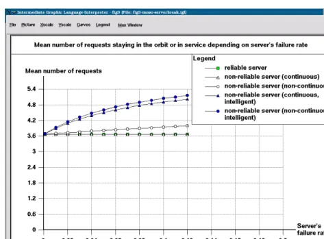
In Figures 1–3 we can see the mean response time, the overall utilization of the system and mean number of calls staying in the orbit or in the service for the reliable and the non-reliable retrial system when the server’s failure rate increases.
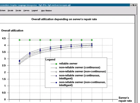
In Figures 4–6 the same performance measures are displayed as the function of increasing repair rate. The input parameters are collected in Table 3.
3.3. Comments
In Figure 1, we can see that in the case when the request returns to the orbit at the breakdown of the server, the sources will have always longer response times.
Although the difference is not considerable it increase as the failure rate increase.
The almost linear increase in E[T] can be explained as follows. In the blocked (non-intelligent) case the failure of the server blocks all the operations and the response time is the sum of the down time of the server, the service and repeated call generation time of the request (which does not change during the failure) thus the failure has a linear effect on this measure. In the intelligent case the difference is only that the sources send repeated calls during the server is unavailable, so this is not an additional time.
In Figure 2 and Figure 5 it is shown how much the overall utilization is higher in the intelligent case with the given parameters. It is clear that the continued cases have better utilizations, because a request will be at the server when it has been repaired.
In Figure 3 we can see that the mean number of calls staying in the orbit or in service does not depend on the server’s failure rate in continuous, non-intelligent case, it coincides with the reliable case. It is because during and after the failure the number of requests in these states remains the same. The almost linear increase in the non-continuous, non-intelligent case can be explained with that if the server failure occurs more often the server will be idle more often after repair until a source repeats his call.
In Figure 4, we can see that if the request returns to the orbit at the breakdown of the server, the sources will have longer response times like in Figure 1. The difference is not considerable too, and as it was expected the curves converge to the reliable case.
In Figure 6, it can be seen that the mean number of calls staying in the orbit or in service does not depend on the server’s repair rate in continuous, non-intelligent case, it coincides with the reliable case like in Figure 3. It is true for the non- continuous, non-intelligent case too, which has more requests in the orbit on the average because of the non-continuity.
4. Conclusions
This paper introduced some recent performance modeling tools of well-known research centers of famous universities. In Section 3 a finite-source homogeneous retrial queueing system was studied with the novelty of the non–reliability of the server. The MOSEL tool was used to formulate and solve the problem, and the main performance and reliability measures were derived and analyzed graphically.
Several numerical calculations were performed to show the effect of server’s break- downs and repairs on the mean response times of the calls, on the overall utilization of the system and on the mean number requests staying in the orbit or in service.
Figure 1: E[T]versus server’s failure rate
Figure 2: UO versus server’s failure rate
Figure 3: M versus server’s failure rate
Figure 4: E[T]versus server’s repair rate
Figure 5: UO versus server’s repair rate
Figure 6: M versus server’s repair rate
References
[1] Almási, B., Roszik, J.and Sztrik J., Homogeneous finite-source retrial queues with server subject to breakdowns and repairs, Mathematical and Computer Modeling 42 (2005) 673–682.
[2] Barner, J.andBolch, G.,MOSEL-2-Modeling, Specification and Evaluation Lan- guage, Revision 2, Proceedings of the 13th International Conference on Modeling Techniques and Tools for Computer Performance Evaluation, Performance TOOLS 2003, Urbana-Champaign, Illinois, (2003) 222–230.
[3] Begain, K., Bolch, G.andHerold, H.,Practical performance modeling, appli- cation of the MOSEL language, Kluwer Academic Publisher, Boston, 2001.
[4] Begain, K., Barner, J., Bolch, G. and Zreikat, A., The Performance and Reliability Modelling Language MOSEL and its Applications, International Journal on Simulation: Systems, Science, and Technology 3 (2002) 69–79.
[5] Derisavi, S., Kemper, P., Sanders, W. H. and Courtney, T., The Möbius state-level abstract functional interface, Performance Evaluation 54 (2003) 105–128.
[6] Falin, G. I.andTempleton, J. G. C.,Retrial queues,Chapman and Hall, Lon- don, 1997.
[7] Haverkort, B. R., Rindos, A., Mainka, V.andTrivedi, K.,Techniques and Tools for Reliability and Performance Evaluation: Problems and Perspectives, Sev- enth International Conference on Modelling Techniques and Tools for Computer Performance Evaluation, Vienna, Austria (1994) 1–24.
[8] Haverkort, B. R. and Niemegeers, I. G., Performability modelling tools and techiques, Performance Evaluation 25 (1996) 17–40.
[9] Wüchner, P., de Meer, H., Barner, J.and Bolch, G.,MOSEL-2 - A Com- pact But Versatile Model Description Language and Its Evaluation Environment, Proceedings of the Workshop: MMBnet’05, University of Hamburg, Germany, 2005.
János Sztrik Faculty of Informatics University of Debrecen P.O. Box 12
H-4010 Debrecen Hungary
Che Soong Kim
Department of Industrial Engineering Sangji University
Wonju, 220-702 Korea

![Figure 1: E[T ] versus server’s failure rate](https://thumb-eu.123doks.com/thumbv2/9dokorg/1218823.92109/13.714.139.613.117.463/figure-e-t-versus-server-s-failure-rate.webp)