PRINCIPAL COMPONENT ANALYSIS IN NEGATIVE INTEREST RATE ENVIRONMENT
Milan LAZAREVIĆ
(Received: 11 December 2017; revision received: 4 May 2018;
accepted: 13 September 2018)
Principal Component Analysis (PCA) is a risk management technique which is, due to the conse- quences of multicollinearity, particularly suitable to describe the yield curve. Its fi nal results in this segment are presented through three main factors: shift, slope and curvature. They express predic- tive trajectories and explain over 95% of variability under normal market conditions. The main goal of this paper is to assess whether the established behavioural patterns are observable in the presence of negative interest rates. The EU bond market was used as an empirical basis with respect to the reactions of the European Central Bank and the establishment of negative reference interest rates in the assessed period. The algebraic properties of the principal components in the presence of negative interest rates correspond to the determined directions of movement, except that the slope and curvature have different signs given their diametrically opposite trends. The percentage of vari- ability explained with the help of PCA is lower compared to the normal market conditions and if an equivalent level of approximation is required, it is necessary to include a fourth factor in PCA. This factor is, due to its properties, aptly named oscillatority. An implicit conclusion of our research is that the duration in the conditions of negative interest rates has less useful power in managing the interest rate risk of individual instruments.
Keywords: Principal Component Analysis (PCA), negative interest rates, interest rate risk, yield curve, correlation matrix
JEL classifi cation indices: C38, E43, G32
Milan Lazarević, analyst, Pavlović International Bank ad, Bijeljina, Bosnia and Herzegovina.
E-mail: milan.lazarevic@pavlovic-banka.com
1. INTRODUCTION: PCA AS A RISK MANAGEMENT TOOL
Principal Component Analysis (PCA) is a technique to describe multiple vari- ables using a smaller number of components. It is based on the assumption that multiple variables can be approximated using a small number of components, as there are common forces that simultaneously affect all of them. Due to such feature, PCA ideally fits into the risk management philosophy since the exposure to multiple variables, or risk factors, can be described using only a few principal components.
According to Jorion (2007), there are two basic dimensions that affect the risk of a position, which are its exposure and volatility. The exposure is classified as an internal parameter, since the entity may influence it through its business deci- sions, whereas the volatility is primarily of an exogenous type. Therefore, the key to risk management is precisely in the correct description of volatility. For the portfolio, it is expressed through a matrix of variance/covariance, i.e. through a matrix of correlation, as established by the Markowitz (1952) portfolio theory.
If it were to be applied rigidly, technical difficulties would swiftly occur due to the necessity to determine all cross-covariances/cross-correlations of variables or risk factors. This is a commonly known problem that affects the economic mean- ingfulness of the matrix, and it is overcome by approximations through multifac- torial models, on the basis of which the number of parameters required for inputs in the calculations is reduced. There are two basic approaches to selecting factors (Jorion 2007). One is based on the use of expert judgement, whereas the second approach is based on the application of statistical techniques in the form of PCA and factor analysis which should objectively approximate the risk positions.
Interest-sensitive positions are influenced by the movement of market interest rates that construct the yield curve. On the one hand, the problem is the multitude of interest rates, which significantly aggravates the management of positions that are subject to interest rate risk. On the other hand, it is clear that in one market, interest rates should have approximately the same trajectory. In such situations, PCA imposes itself as a powerful alternative as it is by its nature suitable only for those variables in which the phenomenon of multicollinearity is present (Bessis 2011). This was first accepted by Litterrman – Scheinkman (1991) as well as by Steeley (1990) in their papers. They concluded that there are three extremely predominant factors that can describe the entire movement of interest rates at a certain market. These are the level, slope and curvature, designated as the princi- pal components. Since the emergence of these papers, PCA in finance has been related to its application on the interest rates. PCA results are very similar when applied in any market (Hull 2010). For example, papers relating to the Canadian market (Bolder et al. 2004) or the Spanish market (Soto 2004) bear the same mes-
sages as established in the initial introduction of PCA in the sphere of depicting the yield curve. The paper by Soto is also important for another reason, which is its capability to analytically prove the advantage of PCA as opposed to one- and two-factor models. One of the more interesting areas of finance that features the application of PCA is the paper by Feeney – Hester (1964), where this technique was used at stock prices and returns for the construction of a stock exchange pseudo index. The logic is, of course, the same, whereas the stock market is used as a medium instead of the bond market. One of the most important papers on the practical application of PCA in risk management is the paper by Frye (1997). It explains the application of the so-called Factor-Based Scenario Method (FBSM) that uses PCA results in constructing a scenario of interest rate movement and their returns influencing the portfolio performance. A specific stress shock is ob- tained in the form of possible negative results on the value of the portfolio, which makes FBSM the means of determination of Value-at-Risk (VaR).
The current economic conditions in the EU bond market, which is placed in the focus of our analysis, are characterized by the presence of negative interest rates.1 Such a phenomenon can be perceived as a specific economic phenom- enon and the causes of which are found in the monetary policy of the European Central Bank (ECB). This situation was intrinsic in most of the developed world markets as a result of the global economic crisis of 2007. Such monetary policy got a new literary name – Negative Interest Rate Policy (NIRP). The issue of inflation in the Euro zone was additionally emphasized due to the influence of the deflationary spiral. According to the empirical findings of Bech – Malkhozov (2016), the transmission of monetary policy through negative interest rates has the same effect on interest rates at the money market as is the case with positive interest rates.
This is not the first case when negative interest rates appeared. A similar situ- ation was present at the Japanese market in the 1990s, where the explanation of this phenomenon was found in the distinction between nominal and real inter- est rates (Mishkin 2004). The negative monetary policy rate contributes to the downward adjustment of the real rates, thus directly affecting the flattening of the yield curve. The direct transmission effects of the NIRP in the European mar- ket in terms of increasing the credit expansion of households can be classified as successful and its further progress is therefore expected (Jobst – Lin 2016).
The inverse yield curve is one of the recession indicators that has been empiri- cally analysed by Chinn – Kucko (2015). Their conclusions are that, although the
1 The expression “negative interest rates” implies that they are not negative for all maturity periods. Wherever this term is used, it includes negative and extremely low interest rates, as well.
predictive power of the yield curve weakened after 1990, it can still be used as a means of indicating the upcoming recession period. For our research, the case of Japan is particularly interesting as it features the Zero Lower Bound (ZLB) period of its monetary policy, significantly reducing the correlation between the yield curve and economic activity.
By contrast, in order to achieve its objectives in similar extreme market con- ditions and to bring down the yield curve, the ECB had to implement uncon- ventional measures of non-monetary policy (Szczerbowicz 2015). The three in- novative solutions were: (i) the introduction of zero deposit rate; (ii) fixed-rate full-allotment procedure (FRFA), and (iii) the three-year refinancing operations (three-year LTROs). Asset purchase programs were imposed as additional crisis management mechanisms. These are particularly important from the perspective of our research as they directly influenced the yields of the government bonds, with the given program of Securities Market Programme (SMP) and its successor program – Outright Monetary Transactions (OMT).
The performance of monetary policy was not only reflected in the control of short-term interest rates, but also in the way in which the central bank man- aged the expectations (Leombroni et al. 2017). They managed to decompose the changes in the Euro zone yield curve into two key dimensions. The first dimen- sion affects the short end of the yield curve, and thus, is categorised as target rate shocks, that is referring to the news on the ECB policy rate level to be considered as a short-term component with direct effects. The second dimension contains an integrated long-term component and is called communication shocks – i.e news on the future direction of the ECB’s monetary policy. The target rate shocks have a significant impact on short-term interest rates and the translation of their im- pact weakens with the increase of the maturity. Apart from the short-term interest rates, the communication shocks have a significantly higher rate of explained variability compared to the target rate shocks indicating that expectation and communication management has a greater impact than changing policy rates. As for the sovereign yields, the effect of the target rate shocks generally decreases with increasing maturities, whereas it becomes clear that they have the highest influence on intermediate maturities.
Following the year 2012, ZLB transcended into Effective Lower Bound (ELB) during 2014, which was the subject of research from Wu – Xia (2017) as the ECB decided to effectively implement NIRP. Such boundaries are further supplemented by Cœuré (2016), who adds the terms Economic Lower Bound, which implies negative effects on the banking industry and the achievement of a situation in which further reduction in rates does not provide stimulus to the economy, as well as representing the ultimate cap of progression of the negative
interest rates – Physical Lower Bound, where transactors perform hoarding of cash. Wu and Xia, through their empirical Euro zone market analysis also found that short-term rates are primarily influenced by monetary policy. The paradoxi- cal situation of particular interest is that the long-term rates are under even greater influence of monetary policy than the short-term ones. In order to describe the above-mentioned phenomena, Wu and Xia prepared a new shadow-rate term structure model (SRTSM) that was analytically elaborated in their innovative paper in 2018. It presented a much more complicated architecture of the short end of the yield curve with three possible historical scenarios. The introduced novel- ties meant that the model featured an integrated component of the expectations of economic transactors on the future trend of interest rates. This analytical upgrade, together with the time-varying lower bound of the monetary policy rate provided for the best fit of their SRTSM as opposed to their other models. Two indica- tors of monetary policy were introduced - one being a short-term one and refer- ring to the current change in the monetary rate, whereas the other representing a long-term vision and related to future monetary policy. Through such setting, the SRTSM managed to anticipate reductions of the ECB deposit rate sooner than the Bloomberg survey, thus proving that the yield curve contains significant informa- tion power on the movement of macroeconomic aggregates and monetary policy.
Its use, due to such significant predictive power, can be tested on the hypothetical reactions of the ECB.
The objective of this paper is to examine whether the characteristics of the principal components have changed in the conditions of prevalence of negative interest rates. All the results made to this day with respect of PCA application in the field of interest rates, even dating back to the aforementioned pioneering papers by Litterman – Scheinkman (1991) and Steely (1990), have shown that the principal components exhibit similar features in all markets. In other words, an analytical question is asked as to whether the behavioural pattern of the principal components is changing under the conditions of negative interest rates or it may retain the same characteristics. To the best of our knowledge, nobody has dealt with this topic so far.
The remaining part of the paper is organized as follows. Section 2 provides theoretical preferences of the problems describing the application of PCA at the interest rate market. Section 3 explains the data that will be used as an empiri- cal basis. Sections 4 and 5 are the essential segments of the paper in which the respective concepts are applied and the empirical results are presented. The last, Section 6 summarises the conclusions drawn from the previous analysis.
2. THEORETICAL BACKGROUND OF THE PROBLEM:
FOCUS ON CORRELATION MATRIX
PCA is a means of simplification with the goal of reducing the number of varia- bles observed thereby accelerating the decision-making process. The cornerstone of the PCA algorithm is the correlation matrix and the principal components that are extracted through its analysis. Essentially, PCA can also operate based on the correlation and covariance matrix. The choice between them does not materi- ally affect the results in individual cases. However, according to Jolliffe (2002), in practical application, PCA is usually applied to the correlation matrix as the results are directly comparable to this matrix. As with all other applications in statistics, the covariance matrix is handicapped in a way that the variables within are not measured on the same scale, whereas in the correlation matrix they are brought into the same level. Lardic et al. (2003) also recommend the use of a correlation matrix when it comes to the application of PCA in describing interest rates. However, PCA is not as usable as most of the conventional statistical tools in terms of hypothesis testing. Standard statistical tests are limited in terms of practical use as the PCA is primarily used to investigate data rather than to verify pre-defined hypotheses (Jolliffe 2002). As it was also stressed in Frye (1997), explaining the analogy of PCA and regression analysis, that PCA is an iteration apparatus to provide a best fit. In other words, there is no need for any assump- tions nor for the pre-selection of regressors, but the components obtained are the results of the calculation itself. That is why it is possible to claim that this statistical technique is quite specific precisely due to such facelessness of the components since they are produced as the main output.
As for the yield curve, the subjects of observation are the interest rates for different maturity periods, whereas the other dimension is represented by their values over time, thus creating a time series. Such movements of interest rates are used to generate the correlation matrix Σ, which is the basis for PCA calcula- tions. As in other applications of statistical conclusions, it is labelled in terms of sample parameters that assess the actual values of the population. As far as this application is concerned, PCA does not differ in any way from the usual statisti- cal techniques. Matrix Σ is presented in a typical manner, through correlation coefficients between interest rates and different maturity periods:
(1)
11 1
21 2
31 32 3
1 2
1 1
1
n n n
n n
ρ ρ
ρ ρ
ρ ρ ρ
ρ ρ
Σ
The main idea is to find the links between the interest rates in order to locate the principal components that can describe their movement. They are found by determining the characteristic values of the matrix, i.e. algebraically perceived, they represent eigenvalues /eigenvectors of Σ. Their calculation begins with the procedure of determining the scalar of λ – eigenvalue and nonnegative vector x – eigenvectors of matrix Σ, which satisfy the following equation (Rencher 2002):
λ
Σx x (2)
The final calculation of λ and x implies solving a characteristic equation:
Σ λI x
0 (3)Thereby, it is important to stress that their orthogonality (x′x = 1) is also achieved, meaning that the effect of each principal component is isolated separate- ly. The singular value decomposition procedure is applied, on the basis of which the matrix Σ is decomposed, with λ and x having the key role in the process :
λ
Σ x x' (4)
This technique allows obtaining a total variance through the aggregation of variation of the principal components (PCs), i.e. their eigenvalues. Thus, an an- alytical apparatus is obtained which implies that the first principal component (PC1) is the component with the highest eigenvalue and the correspondent ei- genvector, the next component (PC2) has the next highest eigenvalue and so on.
By placing a PC variance into a relation with the total variance, it results in the percentage of variability it explains. The aforementioned orthogonality allows for a simple aggregation of the PCs, thereby accumulating the percentage of ex- plained variability. This is precisely the key feature and allows the use of only a few PCs instead of using all the variables. In other words, the matrix Σ can be reduced without the great loss of its information power. Algebraically perceived, this procedure determines the rank Σ (r), which represents the number of PCs with r < n, where n represents the number of variables (Jolliffe 2002). It means that some columns of Σ are not completely independent and can be filled by a linear combination of other columns which allows their approximation through these independent columns. In specific applications of empirical analysis it was found that the first three PCs describe more than 95% of the variability of interest rate movements. They are called PC1 – shift (alternate name: level), PC2 – slope (alternate name: twist) and PC3 – curvature (alternate name: bowing), which can be altogether called SSC, in terms of their acronyms. Their movements are, as al- ready noted, similar in almost all markets when there are no stressful conditions.
The practical implication of SSC is that instead of exposure to all interest rate sensitive positions, exposure can be reduced to only those three PCs. In other
words, the matrix Σ is reduced to only three components and they are sufficient to adequately approximate the entire yield curve. This is a direct consequence of the high level of multicollinearity existing between the movements of interest rates with different maturities. Empirically, this is proven by Σ with extremely high positive values of all the correlation coefficients included within. The features of the correlation matrix of the forward interest rates are described as follows by Salinelli – Sgarra (2006):
a) interest rates at different maturities are always positively correlated;
b) the correlation coefficients decrease when the distance between the indices increases: this is a far obvious consequence of the decreasing degree of correla- tion when the variables are more distant in time; and
c) the previous reduction in the correlation between variables corresponding to the same difference in the indices tends to decrease as the maturities of both the variables are greater.
Since the matrix Σ is symmetrical to the properties of positive definiteness in its quadratic form, all eigenvalues are positive. For its greatest eigenvector, i.e.
shift, the Perron-Frobenius theorem is of crucial importance (Rencher 2002): “If all the elements of the positive definite matrix are positive then the elements of the first eigenvector are positive.” Here, one takes into account the usual conven- tion that eigenvectors are ranked by size, which is important from the aspect of the application of PCA. Perron-Frobenius theorem fully explains the character- istic values of shift and why it is always expressed positively in the movement of interest rates (Lord – Pelsser 2007). Here, we could make an analogy with the concept of duration that marks the sensitivity of instruments to the parallel changes in the interest rate. For this reason, shift is the main component that ex- plains by far the highest percentage of variability.
The behaviour patterns of the remaining two principal components, slope and curvature, are proved by the properties of Σ, which based on its characteristics and under certain circumstances can be classified as a Totally positive matrix as well as a member of the subgroup of Oscillating matrices. Detailed evidence and explanations can be found in Salinelli – Sgarra (2006, 2007) and Lord – Pelsser (2007). This is very important for describing the SSC given the algebraic prop- erties of the aforementioned matrix types and the application of the positivity theory. In this sense, they are characterized by the function of their eigenvectors.
It is necessary that the matrix Σ is completely positive and that there is some power that makes it strictly positive. It is essentially reduced into the analysis of third-order minors as the first three eigenvectors and their submatrices of Σ are required. In other words, a sufficient precondition for the correlation matrix to show the SSC is to be of the oscillatory order 3. Algebraically, it is expressed through the following conditions (Lord – Pelsser 2007):
a) Σ is TP3 (totally positive of order 3);
b) Σ is non-singular; and
c) For all i = 1,...,N–1 we have ρi,i+1 > 0 and ρi+1,i > 0.
It is clear that the properties that are universal in these types of matrices are transferred to Σ as well. They help us understand why SSC get such values. First of all, it refers to the oscillatory matrix characteristic that nth eigenvector has ex- actly n–1 sign changes (Lord – Pelsser 2007). Analogy with the SSC is obvious, as shift, being the first PC has no sign change (the first eigenvector, meaning that n = 1 and the sign change is 1–1 = 0), slope has exactly one sign change (PC2, n = 2, sign change is 2–1 = 1) and curvature has two sign changes (PC3, n = 3, sign change is 3–1 = 2). Salinelli – Sgarra (2006) emphasize that the fundamental properties of the correlation matrix are insufficient to ensure that it will have the characteristics of a totally positive matrix, or of the oscillation matrix; however, the inverse relationship is unambiguous in the sense that a totally positive matrix reflects the aforementioned properties.
3. DATA: EU BOND MARKET
Forward rates of bonds from the Euro zone member countries with sovereign rating AAA were used as the basis for the empirical analysis. Data were sourced from Eurostat database, for two periods: 6 September 2004 – 31 December 2007 and 5 June 2014 – 21 September 2017. Data from the forward rate yield curve were used as the basis, instead of those from the zero-coupon rates, in accordance with the conclusions of Lord – Pelsser (2007) based on the criticism of Lekkos (2000).2 The rationale of Lekkos is that on the basis of these data we get a dis- torted picture (overestimation). The key argument is that zero yield represents the average of continuously compounded forward rates.
The observation periods 1Y–5Y, 7Y, 10Y, 15Y, 20Y, 30Y were selected for clearer display of the results in accordance with the principle of parsimony in economic modelling3. Such selection of maturity periods is conditioned by two reasons. First, in a real business environment, there is a predominant interest for shorter maturities, which is why all maturity periods up to 5 years have been se- lected. For longer periods only borderline periods, whose distance increases with
2 He pointed out the inadequacy of PCA’s approach to the yield curves of previous authors, primarily by Litterman – Scheinkman (1991) and Steeley (1990), in terms of choosing a zero- coupon rate.
3 EUROSTAT provides data for all annual maturity periods ranging from 1 to 30 years.
the extension of the observation period, have been selected. Secondly, only the periods of up to 5 years contain negative interest rates.
Two samples on which the PCA concepts will be applied were designated.
One sample was presented by the period of negative interest rates and, given the nature of the research, it was marked as the primary medium for the deduction of conclusions. Alternatively, a sample from the “normal times” was selected at the time when interest rates were in their usual positive values with the intention to have its results used as a comparative foundation to market conditions character- ized by negative interest rates.
3.1. Yield curve in negative interest rate environment
The EU bond market has been characterized by the appearance of negative in- terest rates in the previous period (5 June 2014 – 21 September 2017). This is a direct consequence of the ECB’s monetary policy in response to the latest crisis.
The establishment of a policy of quantitative easing (QE) aimed to drastically lower the market interest rates that should have spurred the new investment cycle.
The reflection that is expected is an increase in economic activity through the rise in GDP with the investments being one of its main constituents.
The objective of monetary policy in this segment is to influence the reference interest rates, which are by their transmission further transferred to the interest rates of market transactors (pass-through mechanism). This chain can be divided into two levels. The first level implies the influence of central bank reference interest rates onto money market interest rates, whereas the second level rep- resents further transmission onto the real economy through the impact on retail loan rates and bank deposits (Aristei – Gallo 2012). Interest rate routing is most pronounced via the corridor set by the ECB in terms of interest rates on deposit facility rate and marginal lending facility rate. The first significant decrease oc- curred on 11 July 2012, when the deposit facility rate was 0%. And, on the same day, the entering of ZLB monetary policy was very unusual, only for it to enter the negative zone on 11 June 2014 amounting to –0.10% (ECB). This negativity is particularly peculiar from the perspective of economic logic, as the interest on assets held with the ECB (deposit facility rate) is thereby paid. In the background, there is clear intention to discourage the banks from holding inactive assets, but to use them for further placement.
Although there were sporadic occurrences of negative 1Y rates in 2012 and 2013 over shorter periods, since the starting period of 5 June 2014, the 1Y rate has been in constant negative values. Following the above date, other rates be- gan to sporadically occur with a negative sign (2Y, 3Y, 4Y and 5Y). Therefore,
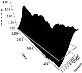
the maximum maturity period that reached negative zone was 5 years. The final cut-off date for which the survey was conducted was 21 September 2017, and in- cluded 840 observations in total. The yield curve movements in the given period are shown in Figure 1.
The graph in Figure 1 is unusual under normal market conditions. Image made in the 3D surface graph best illustrates the events on the yield curve, as a com- plete picture of the events at the bond market is gained. It resembles a hillside that is decreasing in the analysed period in relation to the starting observation point with certain periods of increase in 2015 and 2017 as a reflection of the macroeco- nomic data from the EMU zone. The increasing trend is especially noticeable in 2017. It is particularly interesting that the pedestal of this hill is further deepened in some periods as a result of the increase in negative values and the periods con- taining such negative values. Summary statistics of individual interest rates for the analysed maturity periods in Figure 1 is shown in Table 1.
The first three periods (1Y – 3Y) feature in average a negative value and a neg- ative median. Parameters that directly and indirectly demonstrate the dispersion of data (standard error, standard deviation and range) show a positive correlation with an increase in the observation period, whereby it is evident that the ends of the yield curve (20Y and 30Y) have the aforementioned parameters considerably smaller compared to the periods from the middle of the yield curve.
Figure 1. Yield curve (forward rates) of EMU zone countries with AAA rating (negative interest rates sample)
Source: Eurostat.
3.2. Yield curve in the “normal times”
The unusual movements from the above sub-section should be compared with those present in normal market conditions, that is, in periods when all interest rates are positive and none of them intrudes into the negative zone. For this rea- son, the best approach would be to select, but this time in an opposite direction, an extreme situation on the market when the interest rates were at a high level.
The period prior to the last great crisis characterized by the “overheating” of the economy of the EMU zone acts as a logical choice, directly influencing the growth of all interest rates.
Taking into account the above, the period starting on 6 September 2004 was selected as the second sample, since this was the first date for which Eurostat published the requested data. The last selected date was the end of 2007, which marks the end of “good times”4. Thereby, a second sample of a total of 853 obser- vations was created, thus achieving the balance in the amount of data compared to the first sample. Its values are shown in Figure 2.
4 This is the period marked by the annual real Euro zone GDP growth rates of over 3%. More precisely, the last two years within the observed range featured the following percentage val- ues, in 2006: –3.2% and 2007: –3.0% (Eurostat).
Table 1. Summary statistics of forward interest rates of AAA rating EMU zone member states (Negative interest rates sample)
Parameter 1Y 2Y 3Y 4Y 5Y 7Y 10Y 15Y 20Y 30Y
Mean –0.441 –0.351 –0.109 0.217 0.557 1.127 1.613 1.821 1.762 1.555 Standard
error (%) 0.91 0.96 1.05 1.20 1.37 1.70 2.07 2.16 1.74 1.20
Median –0.455 –0.420 –0.140 0.170 0.540 1.140 1.570 1.740 1.750 1.590 Standard
deviation (%) 26.27 27.79 30.57 34.71 39.59 49.13 59.96 62.49 50.34 34.92 Kurtosis –1.456 –1.326 –0.835 –0.323 –0.060 0.164 0.336 0.100 –0.296 –0.256 Skewness –0.020 0.157 0.333 0.302 0.256 0.350 0.594 0.594 0.120 –0.272 Range 0.950 1.130 1.320 1.640 1.920 2.400 2.810 2.790 2.200 1.680 Minimum –0.960 –0.900 –0.650 –0.460 –0.220 0.190 0.550 0.720 0.740 0.750 Maximum –0.010 0.230 0.670 1.180 1.700 2.590 3.360 3.510 2.940 2.430 Source: Author's calculations.
Note: Descriptive statistics for forward rates of AAA rating EMU zone member states in the period from 5 June 2014 to 21 September 2017. This period characterizes presence of the negative interest rates.
4. EMPIRICAL RESULTS: APPLICATION OF PCA IN THE PRESENCE OF NEGATIVE INTEREST RATES
4.1. Correlation matrix in conditions of negative interest rates
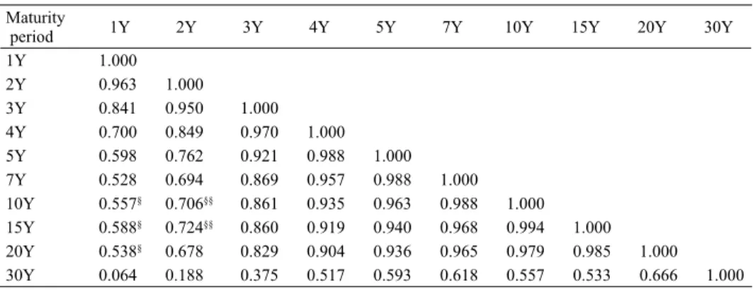
The initial step of our study was the construction of the empirical correlation ma- trix Σ. The calculations were done using Microsoft Excel software, with the data analysis add-on modules. The results are shown in Table 2.
By checking the compliance of the empirical matrix Σ with the characteristics of the immanent correlation matrices of the yield curves listed in Section 2, it is noted that there are certain anomalies in relation to values in normal market con- ditions. The first requirement of multicollinearity, which implies the presence of solely positive correlation coefficients, has certainly been satisfied and it is still evident. However, the constant decreasing values over time distance show non- conformities in 1Y and 2Y. As highlighted in Table 2, unconventional movements in the 1Y correlation coefficient function with expected values are present in the period from the midpoint of the yield curve (10Y, 15Y, and 20Y) while in the 2Y there is nonconformity with 10Y and 15Y. Interpretation of these results suggests that in extremely short periods of time, in the conditions of negative interest rates there are deviations from the usual movement of interest rates. On the one hand,
Figure 2: Yield curve (forward rates) of EMU zone countries with AAA rating (positive interest rates sample)
Source: Eurostat.
it is evident that the interest rate for 1Y is more correlated with the movements of 10Y, 15Y and 20Y than with the interest rate 7Y, which would be its expected trajectory (ρ1Y10Y, ρ1Y15Y, ρ1Y20Y>ρ1Y7Y). On the other hand, as for 2Y, it is an incon- sistency with respect to 10Y and 15Y (ρ2Y15Y, ρ2Y20Y>ρ2Y7Y).
In the previous results, the construction of Σ was based on the level of interest rates. Taking into account only this parameter, a somewhat distorted picture of the correlation status is obtained, as there is an overestimation of value due to the fact that they are non-stationary. Therefore, it is recommended by Lardic et al.
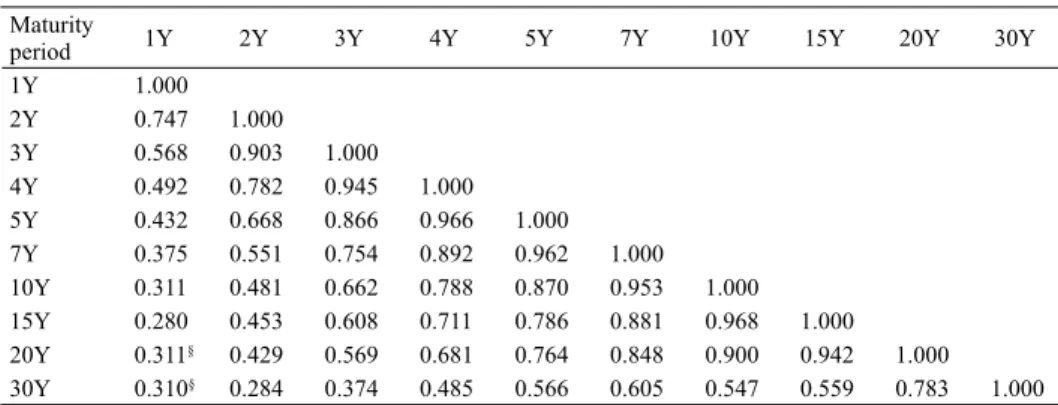
(2003) that the PCA is to be implemented on interest rate changes, since the use of the first differences provides evidence for stationarity of the time series com- prising the yield curve. Such an approach is stressed by other authors in terms of the analytical approach of PCA, for example in Hull (2010). The significance of the shown matrix Σ in Table 2 remains, but due to the described problem of non- stationarity, the further analysis features the use of the first differences instead of the interest rate at levels. The new matrix Σ with such data is shown in Table 3.
Likewise, for Σ as well there is an anomaly for the first differences in the func- tion of decreasing values of the correlation coefficient. This time it is present only for 1Y interest rates and the maturity mismatch has been moved to the last periods (20Y and 30Y). This implies that the 1Y rate is more correlated with 20Y and 30Y rates than with a rate of 15Y (ρ1Y20Y, ρ1Y30Y>ρ1Y15Y). The correlation coefficients in the first difference matrix are lower in relation to the correspondent values in the interest rate level matrix. Once again, the 1Y interest rate is noticeable, with
Table 2. Correlation matrix of forward interest rates (Negative interest rates sample)
Maturity
period 1Y 2Y 3Y 4Y 5Y 7Y 10Y 15Y 20Y 30Y
1Y 1.000
2Y 0.963 1.000
3Y 0.841 0.950 1.000
4Y 0.700 0.849 0.970 1.000
5Y 0.598 0.762 0.921 0.988 1.000
7Y 0.528 0.694 0.869 0.957 0.988 1.000
10Y 0.557§ 0.706§§ 0.861 0.935 0.963 0.988 1.000 15Y 0.588§ 0.724§§ 0.860 0.919 0.940 0.968 0.994 1.000 20Y 0.538§ 0.678 0.829 0.904 0.936 0.965 0.979 0.985 1.000 30Y 0.064 0.188 0.375 0.517 0.593 0.618 0.557 0.533 0.666 1.000 Source: Author's calculations.
Note: Correlation matrix of the forward rates of AAA rating EMU zone member states in the period from 5 June 2014 to 21 September 2017. This period characterizes presence of the negative interest rates.
§: inconsinstency for 1Y maturity (ρ1Y10Y, ρ1Y15Y, ρ1Y20Y>ρ1Y7Y)
§§ : inconsinstency for 2Y maturity (ρ2Y15Y, ρ2Y20Y>ρ2Y7Y)
its correlation coefficients being significantly lower in comparison to the inter- est rate level matrix. Obviously, such negative values of 1Y have caused distor- tions on the market which the transactors could not adapt to in an adequate way.
This is a reflection of the movement of reference interest rates of EURIBOR that are closest to the 1Y rate, i.e. it is closest to the ECB’s rates affecting the pass- through mechanism.
4.2. PCA eigenvectors and eigenvalues in the conditions of negative interest rates The key result of the research is the application of PCA to the set of data de- scribed in Sub-section 3.1. The stability of the results strongly depends on the selection of the time period which has been empirically proven by Soto (2004) in the sense that the rolling-over models perform inferiorily as opposed to the full- period models, due to which the latter approach is applied. Choosing different sub-periods would greatly affect the instability of the results. The modification was made in the sense that the changes (first differences) are taken into account of the issue of non-stationarity. The above can be supplemented with the conclu- sion by Bolder et al. (2004) that daily changes have a decisive impact on the short-term risk and return behaviour for government bonds. Another methodo- logical assumption to be emphasized is the choice between centred or standard- ized changes, i.e. whether PCA is applied on a covariance or correlation matrix
Table 3. Correlation matrix of first differences of forward interest rates (Negative interest rates sample)
Maturity
period 1Y 2Y 3Y 4Y 5Y 7Y 10Y 15Y 20Y 30Y
1Y 1.000
2Y 0.747 1.000
3Y 0.568 0.903 1.000
4Y 0.492 0.782 0.945 1.000
5Y 0.432 0.668 0.866 0.966 1.000
7Y 0.375 0.551 0.754 0.892 0.962 1.000
10Y 0.311 0.481 0.662 0.788 0.870 0.953 1.000 15Y 0.280 0.453 0.608 0.711 0.786 0.881 0.968 1.000 20Y 0.311§ 0.429 0.569 0.681 0.764 0.848 0.900 0.942 1.000 30Y 0.310§ 0.284 0.374 0.485 0.566 0.605 0.547 0.559 0.783 1.000 Source: Author's calculations.
Note: Correlation matrix of the first differences of forward rates of AAA rating EMU zone member states in the period from 5 June 2014 to 21 September 2017. This period characterizes presence of the negative interest rates.
§: inconsinstency for 1Y maturity (ρ1Y20Y, ρ1Y30Y>ρ1Y15Y).
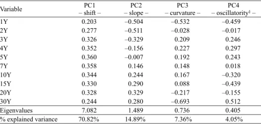
(Lardic et al. 2003). Although the advantage of using the correlation matrix in the general case has already been elaborated, Lardic et al. (2003) give it an additional analytical advantage in applying the yield curve due to the issue of the overrated impact of higher volatility of short-term interest rates. Empirical results showing the PCA and their values under negative interest rate conditions (from sample in Subsection 3.1.) are shown in Table 4. The calculations were made using R software package.
Due to more transparent analysis and assistance in interpreting PCA results, SSCs are graphically depicted in Figure 3.
Comparative analysis of PCA under normal market conditions from previous studies and the one performed under stressful conditions, which imply the pres- ence of negative interest rates, is reduced to a comparison of values of SSC in those two cases. The first thing to notice in the calculated SSC is their consistency with respect to their sign regardless of the presence of negative interest rates. The properties of the oscillatory matrices remain to be effective as the sign change oc- curs under the usual behavioural patterns. It is obvious that the previous analysis of matrix Σ inconsistency in segments described in Sub-section 4.1. did not affect the overall calculations.
The results displayed in SSC vectors, such as in the case of Table 4, act as factor loadings, that is, they indicate the change in interest rates in relation to the change of a specific factor (Hull 2010). Therefore, they are used in the calcula-
Table 4. PCA results in the conditions of negative interest rates
Variable PC1
– shift – PC2
– slope – PC3
– curvature – PC4 – oscillatority§ –
1Y 0.203 –0.504 –0.532 –0.459
2Y 0.277 –0.511 –0.028 –0.017
3Y 0.326 –0.329 0.209 0.246
4Y 0.352 –0.156 0.227 0.297
5Y 0.360 –0.007 0.192 0.243
7Y 0.358 0.146 0.148 0.018
10Y 0.344 0.244 0.167 –0.320
15Y 0.330 0.290 0.088 –0.439
20Y 0.328 0.329 –0.217 –0.155
30Y 0.244 0.280 –0.693 0.512
Eigenvalues 7.082 1.489 0.736 0.405
% explained variance 70.82% 14.89% 7.36% 4.05%
Source: Author's calculations.
Note: PCA result is based on correlation matrix of the first differences of forward rates of AAA rating EMU zone member states in the period from 5 June 2014 to 21 September 2017. This period characterizes presence of the negative interest rates.
tion of VaR, similarly to the case with the FBSM mentioned in Section 1, and as the combination of the influence of factors quantified through factor loadings can construct a scenario of the future impact of changing the specific maturities.
They serve to approximate stressful conditions of changing the specific maturi- ties which an entity is exposed to. The flexibility of the scenario implies making combinations of rise or drop of individual factor loadings, resulting in a wide range of possible movements of the yield curve with a focus on those maturities that are crucial in terms of exposure to the interest rate risk.
Shift, as PC1, shows positive results for all maturities, which is consistent with Perron-Frobenius theorem, which is highlighted in Section 2. It causes all interest rates to increase, with this impact being higher in the middle of the yield curve in relation to its ends. One of the basic premises that all interest rates are influenced by the unique forces that cause them to move synchronized has been fulfilled.
Slope, as PC2, has negative values for maturities up to 5Y, whereas longer ma- turity periods have a positive sign. Interpretation would mean that in the event of an increase in this factor, there would be a reduction in the short-term interest rates, with the opposite effect occurring with the long-term interest rates, i.e. they tend to increase. The most interesting effect comes from the curvature (PC3) due to the increase in the complexity of the yield curve trajectory. The ends of the yield curve (1Y–2Y and 20Y–30Y) are negative, whereas mid-periods are posi- tive (3Y–15Y). In other words, the curvature or twist of the yield curve in terms of the presence of negative interest rates leads to the reduction of short-term and long-term interest rates, whereas the medium-term will increase.
Figure 3. SSC in conditions of negative interest rates Source: Author's calculations.
The cumulative percentage of the explained variability is still high, being over 90% (the exact figure is 93.07%) but such level of explanation is somewhat lower compared to research conducted in normal market conditions ranging from 95%
to 99%. For example, in Litterman – Scheinkman (1991) the explained variabil- ity is 99.50% (PC1 – 89.5%, PC2 – 8.0% and PC3 – 2.0%) and in Frye (1997) it is is 95.7% (PC1 – 83.1%, PC2 – 10.0% and PC3 – 2.6%). It is also noted that the percentage of explained variability of PC1 or shift amounting to 70.82% is significantly lower if compared to the values from previous studies under normal market conditions where the given percentage is at the level of 80–90%. It is im- plicitly concluded that the use of duration as a technique for managing the inter- est rate risk of an individual instrument should be much more careful in case of negative interest rates. The non-linearity of the inverse relationship between the yield and the price of debt securities is much more pronounced. The direct conse- quence of this should be the avoidance of approximations containing integrated assumption of linearity, such as duration, and the use of convexity as an interest rate risk management technique at the level of a single instrument.
If the level of explained variability is to be achieved in the presence of nega- tive interest rates, as in normal market conditions, the applied PCA should be ex- panded further up to the fourth factor. Thereby, the cumulative percentage of the explained variability would increase from 93.07% to 97.02%, therefore achiev- ing the results comparable with previous research. The fourth factor has three changes, the introduction of which increases the utilization capacity, although its impact is complex with respect to the movement of the yield curve. It brings negative properties for the short end of the yield curve (for periods 1Y and 2Y), turning positive from 3Y to 7Y, only to re-enter the negative zone for the periods 10Y – 20Y and finally to emerge as positive at the very end of the yield curve for 30Y maturity. Because of these features of alternating signs, we may call it “oscil- latority”. By integrating oscillatority into PCA, we obtain equivalent results with normal market conditions.
5. APPLIED PCA: “BAD” VS “GOOD TIMES”
The application of PCA under negative interest rates is supplemented with ad- ditional empirical analysis of its properties in normal market conditions on the same medium, i.e, two extreme cases are observed at the EMU market. NIRP thus occurs as a reaction to unfavourable macroeconomic trends that we may call “bad times”. A comparative analysis with the expansion of economic activities, which we can call “good times”, was done for the purpose of applying the given concept to the sample from Subsection 3.2.
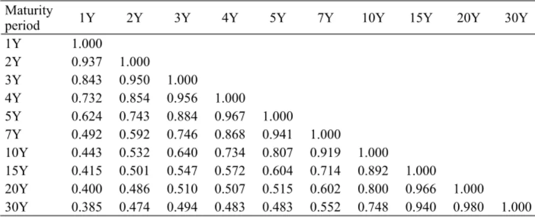
Although the correlation matrix of the levels in “good times” also displays anomalies such as certain discrepancies for periods 1Y–5Y, the first differences show conformity with the established properties of correlation matrices at the in- terest rate market (Table 5). This means that there are no unusual trends in interest rate changes and that there is strong synchronization with various maturities with clear tendencies of direction change.
The results of the PCA application on the sample from “good times” represent- ed as the achieved SSC values are summarized in Table 6. The methodological as- pects are the same as for the application of Subsection 4.2 for direct comparability.
The results of previous research are repeated in the sense that the percentage of explained variability is significantly higher in normal market conditions and according to the results for the period of 2004–2007 amounts to 97.27% for the Euro zone. This confirms the conclusion that in the presence of negative interest rates it is necessary to include a new factor – oscillatority in order to achieve in- creased precision of the use of PCA. Its equivalent utilization is thereby ensured through this inclusion even when negative interest rates with normal market con- ditions prevail on the market. There is still a somewhat greater significance of the shift, which is why the consistency of using the duration concept is a consistent conclusion. A comparison of the obtained SSC results between the application of PCA in “bad” and “good times” is shown in Figure 4.
Table 5. Correlation matrix of first differences of forward interest rates (Positive interest rates sample)
Maturity
period 1Y 2Y 3Y 4Y 5Y 7Y 10Y 15Y 20Y 30Y
1Y 1.000
2Y 0.937 1.000
3Y 0.843 0.950 1.000
4Y 0.732 0.854 0.956 1.000
5Y 0.624 0.743 0.884 0.967 1.000
7Y 0.492 0.592 0.746 0.868 0.941 1.000
10Y 0.443 0.532 0.640 0.734 0.807 0.919 1.000 15Y 0.415 0.501 0.547 0.572 0.604 0.714 0.892 1.000 20Y 0.400 0.486 0.510 0.507 0.515 0.602 0.800 0.966 1.000 30Y 0.385 0.474 0.494 0.483 0.483 0.552 0.748 0.940 0.980 1.000 Source: Author's calculations.
Note: Correlation matrix of the first differences of forward rates of AAA rating EMU zone member states in the period from 6 September 2004 to 31 December 2007. This period characterizes presence of the high positive interest rates.
Table 6. PCA results in the conditions of positive interest rates
Variable PC1
Shift PC2
Slope PC3
Curvature
1Y 0.275 0.356 0.460
2Y 0.311 0.330 0.356
3Y 0.335 0.303 0.086
4Y 0.341 0.254 –0.181
5Y 0.337 0.177 –0.370
7Y 0.331 –0.003 –0.491
10Y 0.332 –0.226 –0.298
15Y 0.313 –0.398 0.084
20Y 0.295 –0.428 0.243
30Y 0.285 –0.429 0.296
Eigenvalues 7.188 1.725 0.814
Explained variance, % 71.88 17.25 8.14
Source: Author's calculations.
Note: PCA result is based on correlation matrix of the first differences of forward rates of AAA rating EMU zone member states in the period from 6 September 2004 to 31 December 2007. This period characterizes pres- ence of the high positive interest rates.
Figure 4. Comparative results of SSC – “bad” versus “good times”
Source: Author's calculations.
The empirical comparative basis provides us with the clear graphical results of the SSC differences in two diametrically opposite states of the Euro zone econo- my. The shift is almost identical in both cases, but it is noticeable that for the near end of the yield curve (up to 3Y) it has higher values when it comes to the normal market conditions, so that in the middle section for maturity in the 4Y–20Y range there is somewhat lower value in comparison to the situation when negative inter- est rates prevail in the market. At the end of the yield curve (30Y) its values are again lower in “bad times”. However, a much more interesting situation concerns the remaining two factors. The slope and curvature have completely reversed tra- jectories in terms of consistency/alteration of their values from positive to nega- tive for different rates of yield curve. This can be explained by the fundamentally opposite tendencies that prevailed in the EMU market in the comparison between the results of two extraordinary cases from Subsections 3.1 and 3.2. Inverting the yield curve which is designated as a recession indicator, as well as the posi- tive inclination of the yield curve in the situations of economic expansion can be analytically proven by the nature of the changes that take place. Their direction is important in terms of whether a tendency can be marked as increasing or de- clining. The analysis of the nature of these changes from the perspective of data movement is shown in Figure 5.
The results obtained were as expected, on the one hand, the data from “bad times” indicate that the changes for all maturities predominantly featured a de- clining trend. On the other hand, the opposite trends were primarily present in
“good times” with the growth being realised for maturities up to 5Y, whereas
Figure 5. Direction of changes in the yield curve movements
a) Negative interest rates sample b) Positive interest rates sample Source: Author's calculations.
all the others feature a higher number of negative changes. This can be one of the reasons why the slope for the yield curve in the sample of positive inter- est rates is positive at first, only to be followed by a turning point at 5Y, which brought the negative values generated thereafter by the slope. It is clear that the described trends and completely different trajectories influenced the shape of the yield curve to be totally opposite to itself, due to which the realized values of the slope and curvature feature completely opposite signs. Such setting has a signifi- cant implication in the practical application of PCA where the business cycle and the environment in which it is used are necessary to be taken into account. The conclusions could be extended to the use of stress testing where the inversion of factor loadings with the slope and curvature could be done in order to witness the effect of a fundamental turn of the yield curve on an entity’s operations. Such method allows us to observe the effect of interchanging “good” and “bad times”, and vice versa.
6. CONCLUSION
Principal component analysis (PCA) is a powerful tool for reducing the observa- tion dimension in a multivariate analysis, which is why it is extremely suitable for active involvement in the risk management process. A segment that is particularly suitable for its application in the risk management sphere is the yield curve that affects interest-rate sensitive positions. Previously, it has been proven through nu- merous researches that almost all markets contain three principal components:
Shift, Slope and Curvature (SSC) that are sufficient to approximate the movement of all interest rates. Regardless of the number of positions that are exposed to inter- est rate risk, all of them can be brought down to only three factors, thus making a significant approximation of their own risky positions. SSC have almost identical characteristics if they are applied under normal market conditions.
The application of the PCA concept in case of negative interest rates is aimed at further examining whether the established patterns continue to exist or there may be certain particularities in the case of negative interest rates. The first pecu- liarity observed in this analysis is that the correlation matrix no longer shows the conformity of characteristics as in normal market conditions. Short-term interest rates have deviant behaviour compared to the expected values. In the case where the correlation analysis is applied to the application of the interest rate level, as for the 1Y and 2Y interest rates, there are anomalies in the sense that there is a higher compliance with the interest rate movements from the middle of the yield curve than to the rates of shorter maturities. If the focus of the analysis is placed
upon interest rate changes, that is, on the first differences of time series, the con- clusion is that only in 1Y there is an anomaly in the sense that its correlation co- efficient is higher with respect to long-term interest rates than the medium-term ones. Obviously, the transactors did not adjust to the new circumstances which were a great surprise with the appearance of negative interest rates, and this par- ticularly affected the extremely short deadlines of up to a year.
Regardless of the presence of negative interest rates and the inconsistency of the correlation coefficient for short-term interest rates, SSCs still show the usual movement patterns in the case of signs of factor loadings. This means that the correlation matrix still has the properties of oscillatory matrices that provide the determined characteristics of the eigenvector influence. Different trajectories of the yield curves in situations when a recession period occurs lead to their in- version, and the period of expansion, in situations when their rise is constantly increasing causes completely opposite behaviour of the slope and curvature. The percentage of explained variability in the PCA process is somewhat lower com- pared to the normal market conditions. In order to achieve the same approxima- tion quality, it is necessary to include the fourth factor, which has been repeatedly named “oscillatority” due to its algebraic properties and fluctuating alterations of its sign. Its introduction provides for the equivalent level of explained variability.
This is particularly pronounced in PC1, forming an implicit conclusion that an additional care should be taken in applying the duration as the risk management technique via a single instrument.
The success of PCA approximation depends on garbage in, garbage out (GIGO) rule that is universal in risk management (Kane et al. 2007). The final results depend solely on the quality of the input in the calculation. Given the applica- tion is executed based on the historical data, the main question asked is whether such movements will remain in the future. This imaging is essential for the ad- equacy of the PCA application process. In this case, this problem is particularly pronounced due to the unusual presence of negative interest rates. Therefore, an additional caution is needed because the fact must be taken into account that with further macroeconomic developments in a period, the need of monetary authori- ties for the determination of negative interest rates will cease. In other words, the proper use of PCA required a necessary recognition of the business cycle status of the market it is used on. Due to the proven diversity of slope and curvature, a particular attention should be paid. The analytical value of such findings can be used in the stress test for interest rate risk in the sense that factor loadings in these PCs are interchanged, and thus allowing the overview of the potential effect of changing the state of economic activity.
REFERENCES
Aristei, D. – Gallo, M. (2012): The Relationship between Bank and Interbank Interest Rates during the Financial Crisis: Empirical Results for the Euro Area. Department of Economics, Finance and Statistics, University of Perugia.
Bech, M. L. – Malkhozov, A. (2016): How have Central Banks Implemented Negative Policy Rates? BIS Quarterly Review, March, 31–44.
Bessis, J. (2011): Risk Management in Banking. John Wiley & Sons.
Bolder, D. – Johnson, G. – Metzler, A. (2004): An Empirical Analysis of the Canadian Term Struc- ture of Zero-Coupon Interest Rates. Bank of Canada: Working Paper, No. 2004-48 .
Chinn, M. – Kucko, K. (2015): The Predictive Power of the Yield Curve Across Countries and Time. International Finance, 18(2): 129–56.
Cœuré, B. (2016): Assessing the Implications of Negative Interest Rates. Speech at the Yale Finan- cial Crisis Forum, Yale School of Management, 28 July 2016.
European Central Bank. Retrieved September 22, 2017, from www.ecb.europa.eu Eurostat. Retrieved September 2017, from ec.europa.eu/eurostat
Feeney, G. J. – Hester, D. D. (1964): Stock Market Indices: A Principal Components Analysis.
Cowles Foundation, Monograph 19, 39: 110–138.
Frye, J. (1997): Principals of Risk: Finding Value-at-Risk through Factor-Based Interest Rate Sce- narios. Risk Publications, Federal Reserve of Chicago.
Hull, J. (2010): Risk Management and Financial Institutions. Pearson Education.
Jobst, A. – Lin, H. (2016): Negative Interest Rate Policy (NIRP): Implications for Monetary Trans- mission and Bank Profi tability in the Euro Area. Working paper, No. 16/172. International Mon- etary Fund.
Jolliffe, I. T. (2002): Principal Component Analysis. Springer Science & Business Media.
Jorion, P. (2007): Value at Risk-The New Benchmark for Managing Financial Risk. McGraw-Hill.
Kane, A. – Marcus, A. – Bodie, Z. (2007): Essentials of Investments. McGraw-Hill.
Lardic, S. – Priaulet, P. – Priaulet, S. (2003): PCA of the Yield Curve Dynamics: Questions of Methodologies. Journal of Bond Trading and Management, 1(4): 327–349.
Lekkos, I. (2000): A Critique of Factor Analysis of Interest Rates. The Journal of Derivatives, 8(1):
72–83.
Leombroni, M. – Vedolin, A. – Venter, G. – Whelan, P. (2017): Central Bank Communication and the Yield Curve. TechReport.
Litterman, R. B. – Scheinkman, J. (1991): Common Factors Affecting Bond Returns. The Journal of Fixed Income, 1(1): 54–61.
Lord, R. – Pelsser, A. (2007): Level-Slope-Curvature-Fact or Artefact? Applied Mathematical Fi- nance, 14(2): 105–130.
Markowitz, H. (1952): Portfolio Selection. The Journal of Finance, 7(1): 77–91.
Mishkin, F. S. (2004): The Economics of Money, Banking, and Financial Markets. Pearson Educa- tion.
Rencher, A. C. (2002): Methods of Multivariate Analysis. John Wiley & Sons.
Salinelli, E. – Sgarra, C. (2006): Correlation Matrices of Yields and Total Positivity. Linear Algebra and its Applications, 418(2-3): 682–692.
Salinelli, E. – Sgarra, C. (2007): Shift, Slope and Curvature for a Class of Yields Correlation Ma- trices. Linear Algebra and its Applications, 426(2–3): 650–666.
Soto, G. (2004): Using Principal Component Analysis to Explain Term Structure Movements: Per- formance and Stability. Progress in Economics Research, 8: 203–226.
Steeley, J. M. (1990): Modelling the Dynamics of the Term Structure of Interest Rates. Economic and Social Review, 21(4): 337–361.
Szczerbowicz, U. (2015): The ECB Unconventional Monetary Policies: Have They Lowered Mar- ket Borrowing Costs for Banks and Governments? International Journal of Central Banking, 11(4): 91–127.
Wu, J. C. – Xia, F. D. (2017): Time-Varying Lower Bound of Interest Rates in Europe. University of Chicago Booth Research Paper, No. 17-06.
Wu, J. C. – Xia, F. D. (2018): The Negative Interest Rate Policy and the Yield Curve. BIS Working Paper, No. 703.