MŰHELYTANULMÁNYOK DISCUSSION PAPERS
INSTITUTE OF ECONOMICS, CENTRE FOR ECONOMIC AND REGIONAL STUDIES, HUNGARIAN ACADEMY OF SCIENCES - BUDAPEST, 2018
MT-DP – 2018/25
Economic convergence and exchange rate misalignments in the European Union
JUDIT KREKO – GÁBOR OBLATH
2
Discussion papers MT-DP – 2018/25
Institute of Economics, Centre for Economic and Regional Studies, Hungarian Academy of Sciences
KTI/IE Discussion Papers are circulated to promote discussion and provoque comments.
Any references to discussion papers should clearly state that the paper is preliminary.
Materials published in this series may subject to further publication.
Economic convergence and exchange rate misalignments in the European Union
Authors:
Judit Kreko research associate
Institute of Economics - Centre for Economic and Regional Studies, PHD Student, Central European University
kreko.judit@krtk.mta.hu
Gábor Oblath senior research fellow
Institute of Economics - Centre for Economic and Regional Studies, Hungarian Academy of Science
oblath.gabor@krtk.mta.hu
October 2018
3
Economic convergence and exchange rate misalignments in the European Union
Judit Kreko – Gábor Oblath Abstract
We investigate (i) the characteristics of real economic and price convergence, (ii) the relationship between economic growth (convergence) and real exchange rate (RER) misalignments within the European Union (EU) during the period 1995–2016. In addition to the relative external price level of GDP, we quantified an alternative indicator for the RER:
the internal relative price of services to goods, as measured from the expenditure side of GDP. We interpreted RER-misalignments as deviations from levels consistent with levels of economic development among EU countries. Regarding real convergence, the “catching up”
of the less developed member states to the more affluent ones within the EU was expressly rapid in terms of relative per capita growth measured at current PPPs; it was less impressive if measured at constant PPPs, and rather modest in terms of relative real GDP-growth. As for price levels and the relative price of services to goods, a rapid convergence could be observed until the international financial crisis, but this process halted in 2008.
Using pooled OLS and dynamic panel techniques, we found that within the EU there is a negative relationship between the contemporaneous sign of RER-misalignment (based on both the external price level and internal relative prices) and economic growth: over- (under-) valuations are associated with lower (higher) growth. This is mainly due to developments in countries operating under fixed exchange rate regimes. Our results indicate that the level of development does not influence the strength of the growth-misalignment relationship within the EU. These results are robust to the applied panel estimation method.
Regarding the external price level, we find that the positive relationship between undervaluation and growth diminishes with increasing size of undervaluation. The aggregate effect of misalignments is significantly negative on both export market shares and the ratio of gross fixed capital formation to GDP: both the competitiveness and the investment channel play an important role in the relationship between growth and RER misalignments. As an extension, we analyse the relationship between growth and the misalignment of wages from productivity levels; “wage-misalignments” are also negatively associated with economic growth.
Although our study carries policy messages – in particular, mild real exchange rate undervaluations are positively, while overvaluations are negatively associated with growth and real economic convergence – the RER is an endogenous variable, which is not under direct policy control. Our results point to the importance of a growth strategy avoiding overvaluation on the one hand, and to the futility of aiming at excessive undervaluation, on the other.
Keywords: real economic and price level convergence; external and internal relative prices;
exchange rate misalignment.
JEL classification: E01, F45, O40; O47; O52; P22; P27
Acknowledgement: The research was supported by the Hungarian National Research, Development and Innovation Office, project No. K-124808. The authors acknowledge the hepful comments of László Halpern, István Kónya and Károly Attila Soós on an earlier draft of our paper. Any remaining errors are those of the authors.
4
Gazdasági felzárkózás és valuta-félreértékeltség az Európai Unióban
Kreko Judit – Oblath Gábor Összefoglaló
Tanulmányunk a reálgazdasági és az árszintfelzárkózás jellegzetességeit, valamint a gazdasági növekedés (felzárkózás) és a reálárfolyam félreértékeltsége közötti összefüggéseket vizsgálja az Európai Unió (EU) tagországaiban az 1995 és 2016 közötti időszakban. A fejletlenebb tagországoknak a fejlettebbekhez történt felzárkózása a GDP/fő alapján folyó vásárlóerő- paritáson mérve kifejezetten gyors volt, mérsékeltebb konstans vásárlóerő-paritáson, és kifejezetten szerénynek bizonyult a GDP reálnövekedése alapján. Az általános árszintek és a belső relatív árak felzárkózását tekintve a 2008. évi nemzetközi gazdasági válságig gyors közeledés mutatkozott, azt követően azonban a folyamat elakadt.
A GDP külső relatív árszintje mellett egy alternatív reálárfolyam-szint mutatót, a szolgáltatásoknak az árukhoz viszonyított belső relatív árát is számszerűsítettük, és a félreértékeltséget a gazdasági fejlettséggel konzisztens szinttől való eltérésként értelmeztük.
OLS, valamint dinamikus panelmódszerekre épülő eredményeink szerint negatív kapcsolat van mind a külső, mind a belső relatív ár alapján értelmezett egyidejű félreértékeltség előjele és a növekedés között: az alulértékeltség gyorsabb, a túlértékeltség lassúbb növekedéssel jár.
Ez az eredmény elsősorban a rögzített árfolyamrendszereket fenntartó országokhoz köthető.
Eltérően a kapcsolódó irodalomban közölt eredményektől azt találtuk, hogy az EU- tagországok esetében a gazdasági fejlettség szintje nem befolyásolja a félreértékeltség és a növekedés közötti kapcsolat szorosságát. A külső relatív árszintre vonatkozó számításaink szerint az alulértékeltség és a növekedés közötti pozitív kapcsolat erőssége az alulértékeltség mértékének emelkedésével gyengül; ez azonban nem mutatható ki a belső relatív ár alapján értelmezett félreértékeltség esetében. Fordított kapcsolatot mutattunk ki egyfelől a félreértékeltség mindkét mutatója, másfelől a piaci részesedés, illetve a beruházási ráta alakulása között, ami azt jelzi, hogy mind a versenyképességi, mind pedig a beruházási csatorna fontos közvetítő lehet a félreértékeltség és a növekedés között. Elemzésünk kiegészítéseként a bér- és termelékenységi szintek közötti összhanghiányként értelmezett félreértékeltség és a gazdasági növekedés összefüggését is megvizsgáltuk; eredményeink szerint a béralapú félreértékeltség is fordított kapcsolatban van a növekedéssel.
Tanulmányuk gazdaságpolitikai üzenete kettős: miközben a túlértékeltséget mindenképpen célszerű megelőzni, az alulértékeltség fokozására irányuló igyekezet sem használ a gazdaság növekedésének.
Tárgyszavak: reálgazdasági és árszintfelzárkózás, reálárfolyam, külső és belső relatív árszint, valuta-félreértékeltség.
JEL-kód: E01, F45, O40; O47; O52; P22; P27
Köszönetnyilvánítás: A tanulmány alapjául szolgáló kutatást az NKFI K-124808 számú projektje támogatta. A szerzők köszönetet mondanak Halpern Lászlónak, Kónya Istvánnak és Soós Károly Attilának a tanulmány korábbi változatához fűzött értékes észrevételeikért. Az esetleges hibákért a szerzőké a felelősség.
5 Table of contents
1. Introduction ... 6
2. Background, motivations and a selective review of the literature ... 11
2.1. Background and motivations... 11
2.2. A selective review of the literature ... 12
3. Key concepts and accounting relationships ... 15
3. 1. Concepts and definition of terms ... 15
3.2. Methodological issues ... 19
3.3. Comparisons over time: current vs. constant PPPs... 22
4. Stylised facts: an overview of the statistical evidence ... 25
4.1. The association between economic development and prices in the EU ... 25
4.2. Aspects and indicators of economic convergence within the EU ... 33
5. Interpreting and measuring real exchange rate misalignment ... 43
5.1. The equilibrium real exchange rate, RER-misalignment and its relationship with economic growth: an overview of the literature ... 43
5.2. Estimation of misalignment... 47
6. The effect of RER-misalignments on economic growth ... 54
6.1. Our approach ... 54
6.2. Results ... 55
7. The effect of misalignments based on the relationship between wage and productivity levels: an extension ... 70
8. Summary and conclusions ... 74
References ... 77
Appendices ... 81
6
“This will in some measure account for the different value of money in different countries; it will explain to us why the prices of home commodities, and those of great bulk, though of comparatively small value, are, independently of other causes, higher in those countries where manufactures flourish.” (David Ricardo)1
1. Introduction
Our study departs from some general observations on economic convergence and developments related to convergence within the European Union (EU), the group of countries in the focus of the present study.
First, and most importantly, while economic convergence – the catching up of less developed countries to the more affluent ones – is not a universal phenomenon, it did characterise the present member-states of the EU over the years 1995 – 2016, the period covered by our work.
The second observation relates to the fact that economic convergence is a complex process, involving a number of interrelated developments. Catching up in terms of per capita real income (measured by per capita real GDP) tends to be accompanied by convergence in productivity (GDP per employed persons or hours worked), price levels, relative prices, nominal and real wages, as well as sectoral shares. The relationships in the focus of the present study are those between real incomes (levels of productivity)2, price levels and internal price structures of countries.
This leads to the third observation: there is a close spatial (cross-county) association between relative real incomes, price levels and price structures within the EU. Higher (lower) levels of real incomes tend to be accompanied by higher (lower) general price levels, as well as higher (lower) relative prices of services to goods. As attested by subsequent rounds of the Penn World Tables (PWT), the positive correlation between real incomes and price levels is a worldwide phenomenon;
this relationship, however, as shown in section 4, holds much more closely within the EU.3
The fourth observation, directly relevant for our study, is that neither the cross-section, nor the longer-term dynamic relationships linking these aspects of economic convergence necessarily hold at a point in time, or in the short-to-medium run for individual countries. This implies that in the case of some countries (or a group of countries) convergence in terms of external/internal relative prices can
“precede” convergence measured by relative real incomes, while other countries (a group therein) may experience the opposite, i.e., that price convergence “lags behind” real economic convergence.
Our study aims to investigate the implications of such “disconnects” between levels (structures) of relative prices and relative real incomes in the process of economic convergence. We shall refer to these disconnects as misalignments of relative external and/or internal relative prices from relative real incomes. Our major interest lies in the relationship between misalignments and economic growth.
The concept of misalignment, naturally, begs the question: what is the point of reference for its empirical interpretation? In other words: what (where) is the “non-misaligned” (or “neutral”)
1 Ricardo (1951), p. 142.
2 Int this section we use the term „real income” as a shorthand for expressing both GDP per capita and GDP per labour input (productivity) measured at purchasing power parity (PPP). Later on we will make a distincion between the two.
3 We compare some global trends revealed by the PWT (2017) with the ones characterising the EU in section 4.
7
level/structure of prices corresponding to the actual state of real economic convergence of a particular country?
The basic notion underlying our study is that within a group of countries consisting of members at considerably different levels of economic development, but closely integrated by trade, capital and labour flows – such is the EU – the overall pattern reflecting the relationship between relative prices and incomes for the group as a whole offers guidance for judging misalignments in individual members of the group. This practically means that in this study the regression line (more precisely:
regressions based on alternative specifications) expressing the relationship between prices and incomes for the EU as a whole is (are) considered to be the benchmark(s) for the empirical interpretation of misalignments in member-states. Positive/negative deviations from the benchmark (residuals of the regressions, alternatively specified) are interpreted as indications of over/undervaluation with respect to the specified benchmark. As discussed and explained later, we rely both on the pooled cross-section data for EU-countries over the period 1995-2016 and on the analysis of five year-periods in our quantitative estimates of misalignments.
However, our actual interest is not simply in quantifying misalignments, but also in investigating the relationship between misalignments and economic growth (real economic convergence). In order to clarify these relationships, we shall apply alternative indicators of both misalignment and real convergence. To check the effect/significance of misalignments within the EU, we complement standard growth equations with indicators of misalignment, similarly to other works on real exchange rates and economic growth. (In section 2.2 and 5.1 we present a selective review of the related literature.)
Our approach is expressly pragmatic with respect to the quantification of misalignment, since we do not have strong prior views regarding the preferred indicator and/or specification (whether the one based on external or internal relative prices is more suitable, or whether indicators with or without controls are superior etc.). Similarly, instead of applying a single indicator for measuring real economic growth/convergence (as usually done in the respective literature), we use several indicators. Beside the change in relative per capita GDP measured at current purchasing power parity (PPP), we shall apply other indicators as well (relative GDP per employed, per capita GDP a constant PPPs, GDP-growth). We expect that this pragmatic approach helps both in identifying the relevant relationships and in demonstrating the complexity of the relationships involved.
The use of alternative indicators for measuring real economic convergence is supported by the observation that the “catching up” of the less developed member states to the more affluent ones within the EU was rather rapid in terms of relative per capita growth measured at current PPPs; it was less impressive if measured at constant PPPs, and rather modest in terms of relative real GDP- growth (i.e., disregarding relative changes in population). Moreover, while the first two indicators point only to a deceleration in real economic convergence, the third suggests an effective halt in convergence after the global economic and financial crisis of 2009. The fact that a significant decline in the absolute size of population in the less developed (Central and East-European) EU member- states has significantly contributed – at least in a technical sense – to convergence in terms of per capita GDP within the EU has not received sufficient attention in the literature. As to be demonstrated in section 4, the overall trend in the world economy has been exactly the opposite, i.e., convergence measured by GDP-growth has been more rapid than if measured by growth in per capita GDP. However, we will also show that, irrespective of the indicator chosen, the speed of real convergence within the EU has been much higher than in the global economy during the period covered by our analysis.
8
Our approach to the issues addressed in this study is similar to Balassa’s (1965) interpretation of
“revealed” comparative advantage. Balassa, skipping the questions concerning the sources of comparative advantage, focused on their effects revealed by countries’ actual specialisation in foreign trade. In a similar vein, we do not dwell on the reasons why less developed countries’ relative prices are lower than those of more affluent ones; we estimate relationships revealed by the statistical data. We continue by applying the indicators of misalignment having turned out to be statistically significant for estimating growth equations in order to clarify: which of the estimated measures of misalignment are relevant with respect to alternative indicators of economic convergence.
Having referred to Balassa, we need to stress that that the term “Balassa-Samuelson- (BS-) effect”, a basic reference in the literature on our subject, has intentionally been avoided in the foregoing.
Though the BS-“effect” is often referred to as a description of the phenomena addressed in our study (i.e., higher levels/growth rates in real incomes are accompanied by higher levels/growth rates in external and internal relative prices), the BS-model is not a description, but one of the possible – often challenged – explanations of the phenomena observed. As to be discussed in section 2, alternative models can also explain the same phenomena from either the supply or the demand side of the economy. Though we touch upon alternative explanations of the observed empirical regularity, our analyses and findings do not depend on the validity of particular models providing explanations. Therefore, throughout our study we apply the terminology suggested by Samuelson (1994): we address the phenomenon as the “Penn effect”, which refers to the statistical source (the PWT) having revealed the empirical regularity, and does not allude to any of its challengeable explications.
Another concept evaded in the foregoing, but to be treated briefly in section 5, is the equilibrium real exchange rate (ERER). The reason for avoiding this notion is that we do not wish to confuse the concept of misalignment of relative prices, as applied in our study, with deviations from alternatively interpreted and measured ERERs. Our interpretation of misalignments is related, but does not necessarily correspond, to concepts involving external and internal macroeconomic balance implied by notions of ERERs.
While avoiding the notion of the ERER, we do rely on the concept of the real exchange rate (RER), and use it for expressing two distinct price-ratios: the external relative price level of GDP and the internal relative price of services to goods; both compared to the average of the EU15. It should be noted that a RER-index is generally interpreted as a nominal exchange rate index divided by a relative price index, while the indicators in our focus are relative price indices divided by exchange rates (the inverse of commonly interpreted RERs). By an “upward” misalignment we mean overvaluation, while a “downward” misalignment means the opposite, i.e., undervaluation throughout our study. Keeping this in mind, we use the terms “relative prices” and RERs in the same sense.
Our study intends to contribute to the literature on the relationship between relative prices (real exchange rates, RER) and economic growth in several respects.
First, and most importantly, the literature on this topic has mainly addressed the experiences of developing countries or a very broad set of countries; just a few studies dealt specifically with the EU, which consists of countries at both high and medium level of income. Our work, in turn, focuses on the experiences of member-states of the EU, a group having been characterised by rapid real economic convergence. However, we shall make comparisons between the EU and a much broader sample, based on the PWT, regarding the relationship between price and income levels, as well as real economic convergence. Our analyses are expected to contribute the clarification of the
9
relationship between real and relative price convergence, as well as the effects of misalignments on real economic convergence.
Second, studies related to our topic generally rely on the external relative price of GDP to express the real exchange rate (RER) and to quantify misalignments. Our work draws on two interrelated, but distinct measures: the external relative price of GDP and the internal relative price of services to goods. In addition, besides drawing on the relationship between relative prices and real income for quantifying misalignments, we also investigate the relationship between relative prices and productivity, measured by GDP per persons employed.
Third, our analyses primarily draw on the Eurostat PPP-database, providing data measured at current PPPs. Most of the related studies, covering large groups of countries, rely on the PWT-database, built on price comparisons at constant PPPs. We believe that for the purposes of our analyses comparisons of price levels at current PPPs is the appropriate approach, since price comparions at constant PPPs are affected by the chioice of the base year.
Fourth, rather than relying on a single indicator for expressing comparative growth performance (i.e., relative per capita GDP at PPP), we consider two additional measures to capture the notion of real economic growth/convergence: the change in per capita GDP and GDP (in itself), both measured at constant prices. The latter two indicators help in identifying the effect of changes in relative prices/composition and population change, respectively, on measures of convergence based on relative real income at current PPP.
Fifth, we amend earlier endeavours to identify the channels through which RER misalignments with a positive/negative sign may hurt/assist economic growth. Besides investments, already addressed in previous studies, we consider the relationship between misalignments and alternative indicators of external trade performance. Since the majority of EU-countries are very open, the “competitiveness- channel” may provide an important link between misalignments and economic growth.
Sixth, beyond results based on estimations of RER-misalignments, we also consider estimates relying on “wage-misalignments”, as interpreted by discreapancies between labour costs and productivity.
Overall, our study is novel in estimating the effect of real exchange rate misalignment across different measures of the RER, the concept of economic growth and that of the level of development. Our results indicate that the contemporaneous extent of real exchange rate misalignment – as interpreted by the external relative price of GDP – is negatively associated with economic growth: a 10% over/undervaluation is accompanied by 0.2-0.7 percentage point lower/higher rate of growth across different specifications. This effect is substantial, considering the fact that the mean annual growth rate of GDP (per capita GDP) was 2.4% (2.3%) in the EU27 over the period covered by our analysis. Misalignments in internal RERs also affect growth, in some cases even more than those in external price levels, highlighting the role of relative prices in resource allocation. A robust finding of the study is that the negative growth effect of misalignment both in external price level and in internal relative prices is mainly attributable to countries operating under fixed exchange rate regime, that is, to Eurozone countries and CEEU countries with pegged exchange rates or currency-board arrangement. This finding is robust to the choice of growth indicator, the measure of relative level of development and the interpretation of the RER.
Our results show that, in contrast with the common finding in the literature, the level of relative development does not influence the strength of the growth effect of misalignments. While external price level-based and internal relative price-based misalignments behave similarly on the aggregate sample, our findings are mixed regarding the symmetry with respect to the size and sign of the
10
misalignment. Specifically, in case of the external relative price level, overvaluation has stronger effect than undervaluation, and while larger overvaluations have an excessively negative growth effect, the positive effect of undervaluation diminishes with increasing size. The growth effect of internal relative price misalignment does not show this pattern.
We address two possible channels through which RER misalignments might influence economic growth: international competitiveness and the investment rate. The aggregate effect of misalignments is significantly negative on both export market shares and the ratio of gross fixed capital formation to GDP. This result indicates that both the competitiveness and the investment channel plays an important role in the growth effect of RER misalignments.
As an extension, we analyse the relationship between growth and the misalignment of wages from productivity levels. Our results indicate that, similatly to RER misalignments, “wage misalignments”
are also negatively associated with economic growth.
Our results capture contemporaneous and one-year lagged effects of RER-misalignments, which are highly relevant for understanding growth and convergence in EU member-states in certain sub- periods of the 21 years covered by our study, but these results do not enable us to draw conclusions about the long-term effects of misaligned price levels and relative prices. It is also important to stress that although our study carries important policy messages – in particular, mild real exchange rate undervaluations are positively, while overvaluations are negatively associated with growth and real economic convergence – the RER is an endogenous variable, which is not under direct policy control.
However, there are several policy instruments for indirectly influencing the RER, even in countries operating under fixed exchange rates. Our results point to the importance of a growth strategy avoiding overvaluation on the one hand, and to the futility of aiming at excessive undervaluation, on the other. Rather than trying to achieve an undervalued RER, governments are advised to focus on improving the quality of institutions. As shown by our estimations, this is one of the important factors that actually matter in the longer term.
We consider the results presented in this paper as a first step in our attempt to clarify the relationship between RER-misalignments and economic growth within the EU. As a next step, it is important to build a theorethical model capable of reproducing the empirical results reported in our study. As a continuation of our work, we also wish to address issues left open in the present study.
Furthermore, the general results of our study need to be ammended by the analysis of individual country-experiences with respect to the evolution of the RER and economic convergence.
The further part of the study is structured as follows. In section 2 we discuss the motivations and background of our work, including a selective review of the related literature. In section 3 we define the basic concepts applied in our analyses. Section 4, relying on these concepts, summarises the stylised facts underlying our econometric estimates. Sections 5 and 6, respectively, present quantitative estimates of misalignments and their effect of different measures economic growth.
Section 7 briefly discusses the issue of wage misalignment; section 8 summarises and draws conclusions.
11
2. Background, motivations and a selective review of the literature 2.1. Background and motivations
Our study builds upon, and contributes to, a rich and prolific strand of research in international economics, namely the literature on the relationship between real exchange rate (RER) misalignments and economic growth.
The notion that a positive correlation exists between levels of (changes in) RERs and levels of (changes in) economic development has a long tradition (see section 2.2.), but has first been statistically demonstrated, accompanied by a model-based explanation, in Balassa’s (1964) seminal article on the reappraisal of the purchasing power parity (PPP) theory of exchange rates. A part of the literature following this thread was occupied by questioning (e.g., Officer, 1976), or verifying (e.g., Kravis and Lipsey, 1983) the existence of the empirical regularity; another part of related works addressed the relevance of the productivity-based explanation provided by Balassa (and, independently from him, by Samuelson, 1964). The discussion on the relevance of the “productivity channel” has continued ever since its exposition.4
An alternative line of research focused on the implications of exchange rate misalignments, in particular, the negative effects of overvaluations (alternatively defined) on economic growth in developing countries.5 Although there were some earlier attempts to combine the observed relationship between price levels and levels of economic development with differences in growth performances (in particular, Dollar, 1992), this line of analysis gained broader professional interest only in the late 2000s (Eichengreen, 2008; Rodrik, 2008).6
While Rodrik’s article, demonstrating the negative/positive effect of overvaluations/undervaluations (interpreted as deviations from the relationship implied by relative price and income levels) on economic growth, received considerable attention and gave an impetus to discussion and further studies, two rarely quoted articles, published almost at the same time, made a similar case, based on analogous theoretical and empirical arguments. Galla (2008) showed that in developing countries misalignments are negatively related to growth, while Podkaminer (2008) presented European examples indicating that extended overvaluations harm economic growth. These examples demonstrate that the issue of RER-misalignment and growth was already “in the air” before the global economic and financial crisis of 2009.
Recent studies (e.g., Habib et al., 2016) also found evidence that misalignments are negatively related to economic growth, but they also found, similarly to Rodrik, that these results hold for less developed countries and do not apply for countries at higher levels of development. This directly leads to the motivations of our research.
One of our important motivations is to check the empirical validity of this commonly accepted finding by observing developments among EU-member states, a group including countries at both high and
4 A thorough review of the related literature is provided by Devereux (2014). For a recent contribution, challenging the notion that higher productivity growth is accompanied by RER-appreciation, see Gubler and Sax (2017)
5 See e.g., Cavallo et al. (1990), Dollar (1992), Razin and Collins (1997), Benaroya and Janci (1999), Acemoglu et al. (2002), Fajnzylber et al. (2002).
6 It should be noted that while several endeavours had been made to explain the underperformance of particular developed economies by RER-overvaluations (see in particular Kaldor [1966 and 1971] on the UK and Corden [1984] on the “Dutch disease”), these interpretations of overvaluations, however, never referred to misalignments of RERs from levels implied by the level of development.
12
medium level of income. Except for Podkaminer (2008), Oblath and Szörfi (2008) and Oblath et al.
(2015), no attempt, that we are aware of, has been made as yet to clarify the relationship between RER misalignments and growth within the EU. The analysis by Podkaminer was somewhat informal;
while the econometric analyses in the latter two studies were rather rudimentary. In particular, they did not address problems involved by potential endogeneity, an issue taken up in the present study.
A second motivation is related to the fact that almost all studies on misalignments and growth focus on the relationship between misalignments as interpreted by deviations of relative price levels of GDP from levels predicted by relative income, i.e., the misalignment of the external RER. This approach does not take into account an important channel through which misalignments may actually work, i.e. the internal relative price of services to goods – which may serve as a proxy for the relative price of non-tradables to tradables.
Third, misalignments, especially their persistence, may be affected by the exchange rate regime. EU- member states participating in the European Monetary Union (EMU) have fixed their nominal exchange rates against each other (Bulgaria and the Baltic countries have implicitly joined the system before actual participation), while other member states have maintained a flexible exchange rate regime. Therefore, the EU is a natural field for investigating the relationship between exchange rate regimes, misalignments and their effects.
Fourth, the speed of real economic convergence of the new EU-member states of Central and East Europe (CEEU) is remarkably different. Do these differences have to do with misalignments as interpreted above, or they are related to other factors? Our study intends to contribute to the clarification of this issue as well.
The last point leads to our fifth motivation: to go beyond the general patterns displayed by the regressions, and look at country-specific experiences. A pattern that holds for a group as a whole does not necessarily apply for individual countries. While observing country-specific developments is certainly not feasible in samples covering more than hundred countries (which is the general case in the related literature), it is not just feasible, but also necessary in the case of the EU. The overall results for the 27 countries should be interpreted in view of the fact they are actually very different.
2.2. A selective review of the literature
In the following we briefly review some of the main contributions to the literature on the relationship between the level of (changes in) the RER and economic development. The literature on the interpretation and measurement of RER-misalignments, as well as on their effect on growth, including details of the estimation methods, is reviewed in section 5.1.
Paul Samuelson (1994) coined the close positive association between the price level of GDP and real per capita GDP the as the “Penn-effect”.7 He – as one of the contributors of the renowned Balassa- Samuelson (BS) model – considered it important 30 years later to distinguish the observed statistical
7 Samuelson referred to the results of international comparisons performed in the framework of the ICP project in which the University of Pennsylvania had a major role. The Penn World Table (PWT) constitutes a major statistical source for worldwide comparisons of real GDP and its components. The data indicate a close positive association between the level of real incomes and relative price levels of GDP. The existence of the Penn-effect contradicts a long-respected notion in international economics, namely the absolute version of the purchasing power parity (PPP) doctrine, which asserts that nominal exchange rates correspond to differences in general price levels. (See Cassel, 1922 on a classical exposition of the PPP-theory.) More precisely, the Penn-effect limits the scope of the absolute PPP-theory of exchange rates to countries at similar levels of economic development. (The Penn-effect implies that the PPP doctrine holds only if differences in real income levels are adjusted for.)
13
regularity (the Penn-effect) from one of its possible explanations, which is the BS-model.8 This important distinction is frequently overlooked, whereby the “BS-effect” is regularly used as a synonym of the Penn-effect. 9
There are several layers of understanding/explaining the Penn-effect; here we refer only to two of these.10 One relates to the following question: the external relative price of which particular GDP- aggregates is chiefly responsible for the observed effect? In this respect, there has been a broad consensus among economists and economic statisticians: the relative price of services (vs. goods or vs. GDP) increases in line with the level of economic development (for earlier works see e.g. Harrod, 1933; Clark, 1940; Fourastié, 1947; Kuznets, 1971).
The second concerns explanations of the observed effect. The most well-known is the BS model, which, building on rather restrictive assumptions, focuses on differences in productivity between goods (an approximation of tradables) and services (an approximation of nontradables). An alternative explanation was offered by Bhagwati (1984), who built his model on differences in factor endowments of the two sectors.
There is, however, a long tradition of explanations from the demand side as well (in particular Fourastié, 1947), but there were several later attempts to this end (see e.g., Bergstrand 1991;
Podkaminer, 2010a). Bergstrand’s argument was based on the assumption that services are “luxury goods” while tradable commodities are “necessities”. Therefore, as national income grows, the demand for nontradable services increases more than that for tradable goods; this leads to an appreciation of the real exchange rate. Bergstrand built an empirically testable model to support this assertion. Using a sample of 21 countries, he distinguished the effects of three possible theoretical explanations for the different real exchange rate levels: his demand-side approach, the Balassa- Samuelson model and the role of different capital-labor endowments based on Bhagwati (1984). His results supported the hypothesis that income has a significantly positive effect on the real exchange rate through higher demand for services even after controlling for productivity and capital-labor endowment differences between the tradable and the nontradable sector. This implies that, beside the supply-side, there is a demand-side channel responsible for the observed regularity.
Regarding the catching-up process in the European Union, Égert (2010) also emphasized the importance of the demand-side channel. He found that the Balassa-Samuelson explanation hardly holds in this sample because of two reasons. First, the productivity growth in services was not far from that in the tradable sector in several new member states of the EU. In addition, the (nominal) share of nontradables is usually low in these countries. As a result, he found that the implied
“Balassa-Samuelson effect” is very weak in new EU member-countries.
Égert also tested the possible drivers of price level convergence with various econometric models.
His results corroborated that the Balassa-Samuelson model was not an important explanation of the process. Regarding the nontradable sector, inflation showed a strong positive correlation with regulated service prices that usually account for a large part of the HICP in the new member states.
House prices and commodity prices also proved to be important drivers of inflation. These results led
8 The term “Balassa-Samuelson model” was suggested by Asea and Corden (1994) in their review of the related literature. For further reviews on alternative tests of the model, see e.g. Égert - Halpern - MacDonald (2005) and Tica and Druzic (2006)
9 For a discussion of the relationship between the Penn and the BS effect, see Pancaro (2011).
10 It should be noted that while the Penn-effect works among countries at considerably different levels of economic development, it does not appear to be significant within the most and the least developed group of countries; see Rogoff (1996) and Hassan (2011) on this point. In section 4 we verify this assertion
14
him to the inference that during the economic catching-up process higher incomes result in changes of the consumption structure of households towards higher quality goods and services. Therefore, price level convergence is due to developments in both the tradable and nontradable sector.
Our study does not deal with alternative explanations; it simply considers the Penn-effect as a statistically firmly based stylized fact, which certainly holds for the EU27 in the period in our focus.11 However, two points have to be made. The first concerns the implications of external and internal relative prices. For the Penn-effect to hold, it is a sufficient condition that the internal relative price of services to goods be higher in more developed countries than in less developed ones, while the external price level of goods may be the same. (Actually, the latter assumption was explicitly made in Balassa’s article.) However, all statistical sources confirm that not only services, but goods are also more expensive in countries at higher levels of development.
This leads to the next point, the “dynamic” Penn-effect (see Ravallion, 2010). What are the major factors responsible for changes in price levels accompanying convergence in real incomes? Several studies have questioned the relevance of the dynamic version of the BS-model, calling attention to the fact that not only the increase in the external relative price of services but also that of goods have a major role in the catching up of price levels (often referred to as “structural inflation”).12 A more important, conceptual issue relates to the nature of the dynamic Penn effect. Over what time horizon do price levels change in response to changes in per capita incomes? Berka and Devereux (2013) show that there is a medium-term correspondence between the cross-country and the dynamic version of the Penn effect. This appears to contradict the findings of Podkaminer (2008), that short-term changes in GDP price levels are unrelated to changes in relative per capita real GDP levels. However, the apparent contradiction may be resolved by the possibility that the longer term relationship is based on “error correction”, whereby deviations from a common “European trend”
may explain short-term changes in relative GDP price levels in Europe. This assumption is confirmed by our analyses. In contrast to Podkaminer (2008), our ECM regressions show that both one-year changes in relative per capita GDP and lagged deviations from the long term relationship influence the one-year change in GDP price level, however, the explanaority power of these variables is rather low (see Appendix, B).
11 As emphasized by Samuelson (1994): “The Penn effect is an important phenomenon of actual history but not an inevitable fact of life.” Bergin-Glick-Taylor (2004) and Taylor and Taylor (2004) demonstrated that, historically, the existence of the Penn-effect is indeed recent: it did not exist in the early 1900-s and evolved (and strengthened) since the middle of the twentieth century.
12 See e.g. Darvas – Szapáry (2008). For a non-technical exposition of the related ideas, see Égert-Podpiera (2008).
15 3. Key concepts and accounting relationships
In this section we first define the key concepts of the paper and clarify their accounting relationships.
Next, we show how some of the analytical categories applied for international comparisons (in particular, goods and services) are related to concepts of the national accounts. The concept of constant-PPP based comparisons will also be clarified.
3. 1. Concepts and definition of terms
3.1.1. Comparative nominal, price and volume levels; external and internal relative prices
In order to clarify the main concepts of our study, we depart from two decompositions of the comparative nominal level of per capita GDP of a particular country. The term comparative refers to the fact that an item/aggregate (e.g., per capita GDP) is being measured relative to another country or to a group of countries; therefore the terms “comparative” and “relative” are to be used interchangeably. The term nominal, in turn, indicates that an item/aggregate is expressed at current prices (i.e., it is not deflated by a price index), irrespective of whether it is measured in national currency units, or converted into a common currency via the current exchange rate.
To connect the conceptual clarification to the quantitative analyses of our paper, our decompositions refer to a member state of the European Union (EU), and the benchmark for the comparisons is the average of the EU.
The decomposition of the “distance” in nominal per capita GDP of member-state i from that of the EU-average is conceptually similar to how nominal changes over time can be decomposed into changes in prices and quantities (volumes) within a particular country.
In country i the change in nominal per capita GDP (measured at current prices) between period t-1 and t can be written as follows:
𝑁𝑔𝑑𝑝𝑡𝑖/𝑃𝑂𝑃𝑡𝑖
𝑁𝑔𝑑𝑝𝑡−1𝑖 /𝑃𝑂𝑃𝑡−1𝑖 = 𝑃𝑔𝑑𝑝𝑡𝑖
𝑃𝑔𝑑𝑝𝑡−1𝑖 ∗ 𝑄𝑔𝑑𝑝𝑡𝑖/𝑃𝑂𝑃𝑡𝑖 𝑄𝑔𝑑𝑝𝑡−1𝑖 /𝑃𝑂𝑃𝑡−1𝑖 (1)
where Ngdp and POP, respectively, indicate GDP at current prices (i.e., nominal GDP) and population size; t and t-1 refer to the current and base period; Pgdp and Qgdp denote the price and quantity (at constant prices) of GDP. The term on the left-hand side indicates the nominal change in per capita GDP in country i; the first term on the right-hand side is a price index (the GDP-deflator), while second is the change in per capita GDP measured at constant prices (a volume index).13
In this study we use Q for indicating real changes over time. We shall use V for expressing real
”distances” between countries at a point in time. The relevance of this distinction will become apparent when discussing changes in real distances over time (section 3.1.).
Turning to international comparisons, formula (1), expressing changes over time, can be interpreted as follows for comparing country i to the EU average in period t (to simplify the expression, the time index is omitted):
𝑁𝑔𝑑𝑝𝑛𝑐𝑖 /𝑃𝑂𝑃𝑖
𝑁𝑔𝑑𝑝𝑒𝑢𝑟𝐸𝑈/𝑃𝑂𝑃𝐸𝑈 = 𝑃𝑔𝑑𝑝𝑛𝑐𝑖
𝑃𝑔𝑑𝑝𝑒𝑢𝑟𝐸𝑈 ∗ 𝑉𝑔𝑑𝑝𝑖/𝑃𝑂𝑃𝑖 𝑉𝑔𝑑𝑝𝐸𝑈/𝑃𝑂𝑃𝐸𝑈 (2)
where Ngdp(i, nc) is the GDP measured at current prices in country i, expressed in national currency (nc), and Ngdp(EU, eur) is the GDP of the European Union at current prices, expressed in euros. The
13 As the expression serves only for illustration, we skip the discussion of methodological issues related to the construction of national price and volume indices.
16
term on the left hand side shows the ratio of per capita GDP in county i, expressed in the country’s currency to that of the EU-average in euros. This ratio, by itself, has no economic meaning whatsoever. However, its decomposition contains two important pieces of information.
The first term on the right-hand side is a spatial (cross-county) price index, while the second one is a spatial volume index. The spatial price index [Pgdp (i, nc)/Pgdp(EU, eur)] is the purchasing power parity (PPP) for GDP in country i, vs. the EU average. It shows how many units of domestic currency has the same purchasing power over a notional unit of GDP in country i, as one euro has over a notional unit of GDP in the average of the EU.
One of the major applications of PPPs is shown by second term on the right-hand side of (2). If the nominal comparative per capita GDP (the left-hand side) is divided by the PPP, the second term on the right-hand side is obtained, namely the volume (the “real” magnitude) of per capita GDP of country i, relative to the EU-average. This spatial volume index is an indication of the relative size of the basket consisting of per capita GDP in country i as compared to the reference country/region. In the following, we refer to this ratio as the volume level index of per capita GDP, to be denoted as VLCgdp.14 This indicator is generally considered to reflect the level of economic development or, alternatively, the level of real income of country i, as compared to the reference country/region.15 The difficulty with interpreting expression (2) is that the numeraire (the unit of currency) in the numerator is different from the one in the denominator. Therefore, both sides of equation (2) have to be divided by the exchange rate (E), in order to decompose the relative nominal level of per capita GDP expressed in a common currency into a spatial price and a spatial volume index. In expression (3), the first term on the right hand side (the PPP for GDP divided by the nominal exchange rate) is the price level index of GDP, to be denoted as PLgdp. It shows how much higher/lower the general price level of country i is relative to the EU-average, expressed in a common currency. The second term on the right hand side is the same as in (2).
[𝑁𝑔𝑑𝑝𝑛𝑐𝑖
𝑃𝑂𝑃𝑖 ] /𝐸 𝑁𝑔𝑑𝑝𝑒𝑢𝑟𝐸𝑈/𝑃𝑂𝑃𝐸𝑈 =
𝑁𝑔𝑑𝑝𝑒𝑢𝑟𝑖 𝑃𝑂𝑃𝑖
𝑁𝑔𝑑𝑝𝑒𝑢𝑟𝐸𝑈/𝑃𝑂𝑃𝐸𝑈 = ⌈1
𝐸∗ 𝑃𝑔𝑑𝑝𝑛𝑐𝑖 𝑃𝑔𝑑𝑝𝑒𝑢𝑟𝐸𝑈⌉ ∗
𝑉𝑔𝑑𝑝𝑖 𝑃𝑂𝑃𝑖 𝑉𝑔𝑑𝑝𝐸𝑈
𝑃𝑂𝑃𝐸𝑈
= 𝑃𝐿𝑔𝑑𝑝 ∗ 𝑉𝐿𝐶𝑔𝑑𝑝(3)
where E and Ngdp(i, eur), respectively, denote the nominal exchange rate and per capita GDP in country i expressed in euros; the rest of the notations are the same as in (2).
To give an idea of the empirical relationship between the three variables in the expression above, Figure 3.1 shows the price level of GDP and the volume level of per capita GDP as a function of the
14 The actual magnitude of VLCgdp depends on the choice of the reference country/region, which differs among different databases. The four important sources containing international real comparisons across countries are the Penn World Tables (PWT, 2016), the World Bank (2016), the OECD (2016) and the Eurostat (2016). The last one is the source of the data used in our quantitative analyses, where the EU average, or the average of a sub-group of countries within the EU can be chosen as a reference.
15 Dividing both sides by [Pgdp (i, nc)/Pgdp(EU, eur)], we get 𝑉𝐿𝐶𝑔𝑑𝑝 = 𝑁𝑔𝑑𝑝𝑛𝑐𝑖 /𝑃𝑂𝑃𝑖
𝑁𝑔𝑑𝑝𝑒𝑢𝑟𝐸𝑈/𝑃𝑂𝑃𝐸𝑈/𝑃𝑔𝑑𝑝𝑛𝑐𝑖
𝑃𝑔𝑑𝑝𝑒𝑢𝑟𝐸𝑈 = 𝑉𝑔𝑑𝑝𝑖/𝑃𝑂𝑃𝑖 𝑉𝑔𝑑𝑝𝐸𝑈/𝑃𝑂𝑃𝐸𝑈 (2𝑏)
17
nominal level of per capita GDP for 27 EU-member states in 2014. For reasons to be explained below, the benchmark, just as in other comparisons in this study, is the EU15, rather than the EU28.16
Figure 3.1: The relationship between nominal and real per capita GDP and the price level of GDP in member-states of the EU in 2014 (EU15 = 100)
Source: Eurostat
Figure 3.1 indicates a very close positive relationship among the three variables within the EU. The lower (higher) the relative nominal per capita GDP (in euros), the lower (higher) is the relative price level (in euros), as well as the relative real per capita GDP (in PPS).17 Moreover, the slope of the regression lines of the latter two variables is practically identical and the lines are very close to each other, suggesting a strong correlation between them. The year 2014 serves for illustration; a similarly close association would show for any other year included in our database covering the period 1995- 2016.18 We shall return to the implications of the phenomenon displayed by Figure 1 later on; now an important amendment to the foregoing decompositions is in order.
We departed from the relationship connecting relative nominal and real per capita GDP and the PPP for (the relative price level of) GDP simply because the international comparison of levels of development (real incomes) is the most frequent application of PPPs. We could also have departed from, e.g., the international comparison of levels of per capita real consumption or real fixed capital formation. Differences between nominal and real levels of these aggregates are just as relevant, as for per capita GDP.
However, with respect to the later items, their own PPPs (price level indices) have to be applied for cross-country comparisons of volumes (levels in real terms). This implies that there is no such thing as “the” PPP, because each component and sub-component of GDP has its own PPP. While, for cross- country nominal comparisons of different items in a common currency there is a single deflator, i.e., the exchange rate, this does not hold for real comparisons between countries. In the latter case, each
16 The EU15 refers to the average of the member-states having belonged to the EU before the enlargement in 2004.
17 The Eurostat uses a special type of PPP, the PPS (purchasing power parity standard). PPS is defined so that 1 PPS has the same purchasing power as 1 euro has with respect to the average of (i) all EU member-states (the EU28), (ii) the EU27 (the EU28 less Croatia), or (iii) the EU15. Depending on the variant of PPS, the average price level of the respective group of countries is the same, whether measured in euro or PPS. Since the time series for certain items expressed in PPS-EU28 are relatively short, our analyses rely on data measured in PPS-EU15.
18 Actually, 2014 is the last year when all of the present member states (less Luxembourg) are taken into consideration in our database applied for empirical analysis. We chose to omit GDP-data for Ireland regarding the years 2015 and 2016 due to a jump of 26 percent in the country’s real GDP in 2015. This increase is related to certain accounting methods of the SNA, rather than to an actual jump in the country’s real economic performance.
0 20 40 60 80 100 120 140
0 50 100 150
PLgdp VLCgdp (pps)
NLC_gdp (eur)
18
item needs to be deflated by its own PPP (price level index) to ensure the comparability of the per capita volumes of the respective items.
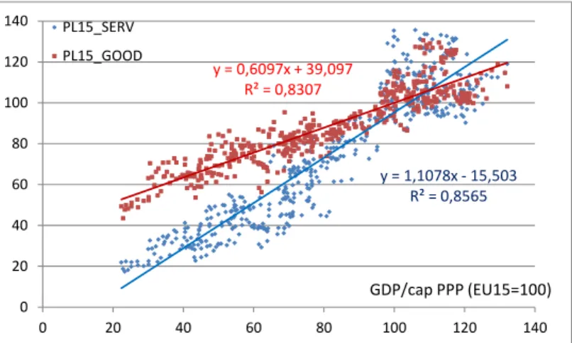
In the following we refer to the price level index of an item (e.g. PLgdp, etc.) as the external relative price of the respective item.
Figure 2 illustrates the importance of distinguishing between the overall external relative price level (PLgdp), and two of its components mentioned above (the external relative price of consumption and that of gross fixed capital formation). The latter two are shown in function of the external relative price of GDP, with the EU15 as a reference.
Figure 3.2: The relationship between the external relative price level of GDP, gross capital formation and consumption in member-states of the EU in 2014 (EU15 = 100)
Source: Eurostat
As shown by the figure, in EU-countries having lower comparative GDP price levels, consumption is relatively cheap and investments are relatively expensive; while the opposite holds for most of the countries having higher GDP price levels. This phenomenon calls attention to the importance of internal relative prices.
3.1.2. Internal relative prices
We define the internal relative price of two aggregates (components of GDP) as the ratio of their external relative prices. The exact name for this ratio should be the “deviation of the internal price ratio from that of the reference region”. However, since there is no such thing as the “internal relative price level” of two aggregates in a particular country, and therefore, at a point in time this ratio can only be interpreted in international comparison, we simply call it an internal relative price.
Still, it has to be kept in mind that this indicator, similarly to any indicator involving international comparisons, depends on the choice of reference region.
For the purposes of our study, the most important internal relative price is that of services to goods, i.e.,
RPsg = PLs/PLg=⌈1𝐸∗𝑃𝑠𝑃𝑠𝑛𝑐𝑖
𝑒𝑢𝑟𝐸𝑈⌉ / ⌈1𝐸∗𝑃𝑔𝑃𝑔𝑛𝑐𝑖
𝑒𝑢𝑟𝐸𝑈⌉=⌈𝑃𝑠𝑃𝑠𝑛𝑐𝑖
𝑒𝑢𝑟𝐸𝑈⌉ / ⌈𝑃𝑔𝑃𝑔𝑛𝑐𝑖
𝑒𝑢𝑟𝐸𝑈⌉
where RP denotes the internal relative price, PL is the external relative price, while s and g, indicate services and goods.19
19 Actually, the reason for choosing the EU15, rather than the EU28 as a benchmark for comparisons in this study is that that PPP-data for the new member states with respect to services and goods are unavailable before the year 2004 with the EU28 average as a reference, while they are available beginning 1999 with the average of the EU15 as a reference.
y = 0,7486x + 25,069 R² = 0,844
y = 1,1091x - 10,2 R² = 0,992
0 20 40 60 80 100 120 140
0 20 40 60 80 100 120 140
PL_gfcf PL_cons
PL_gdp
19
This ratio can either be considered as a proxy of the relative price of non-tradables to tradables (in the spirit of the Balassa-Samuelson model), or as an indicator on its own right (as suggested by the demand-side explanations of the relationship between RPsg and per capita GDP).20 Whatever the status and explanation for the behaviour of RPsg, its relationship with nominal per capita GDP is very similar to that of the external relative price level of GDP (PLgdp) – as shown by Figure 3.
Figure 3.3: The relationship between nominal GDP, the price level of GDP and the internal relative price of services to goods in member-states of the EU in 2014 (EU15 = 100)
Source: Eurostat and own calculations
Figure 3.3, similarly to the two previous figures, shows cross-section relationships relative to the EU15 average for the year 2014. Just as PLgdp, RPsg is also closely positively correlated with per capita GDP; the slopes are similar, but the dispersion around the cross section trend is somewhat larger in the case of the latter.
3.2. Methodological issues
We address three methodological issues related to the interpretation of the internal relative price of services to goods. The first concerns the relationship of the two aggregates behind RPsg with the categories of the System of National Accounts (SNA). The second relates to the aggregation method underlying our data, while the third concerns the analytical vs. empirical relationship between PLgdp and RPsg.
3.2.1. Goods and services vs. SNA aggregates
“Goods” and “services” are analytical categories specifically constructed for the International Comparison Programme (ICP), based on PPPs.21 Since the SNA does not recognise these categories, it should be useful to clarify their relationship with the more familiar aggregates of the national accounts.
The basic identity for the expenditure side of GDP is:
GFCF + dST+ C + NX = GDP (4)
where GFCF, dST, C and NX, respectively, denote gross fixed capital formation, change in stocks, final consumption (private and public) and net exports.
The identity connecting the two analytical categories of the ICP with GDP aggregates (also interpreted from the expenditure side):
GO + SE + NPA + dST + NX =GDP (5)
20 See e.g., Bergstrand (1991) and Podkaminer (2010).
21 See e.g.,Eurostat –OECD (2012) [PPP manual]
y = 0,5854x + 38,498 R² = 0,936
y = 0,5092x + 43,018 R² = 0,8213
0 20 40 60 80 100 120 140
0 50 100 150
PLgdp RPsg
NLC_gdp (eur)
20
where GO, SE and NPA, respectively, denote total goods, total services and “net purchases abroad”
(approximately: the inverse of net revenues from tourism); the rest of the notations are the same as in (4). As shown by identity (5), there are three items driving “wedges” between the sum of goods and services on the one hand, and GDP, on the other: net purchases abroad, changes in stocks and net exports. This implies that the aggregate of goods and services does not correspond to total domestic demand (DD) either, since the latter includes, while the former excludes NPA and dST:
GO + SE + NPA + dST =GDP – NX = DD (5a)
What the sum of goods and services exactly corresponds to (at current prices) is the sum of gross fixed capital formation and final consumption (i.e., domestic demand less changes in stocks) minus net purchases abroad:
GO + SE = GDP – (NPA + NX + dST) = GFCF + C – NPA (5c)
The important point is that the sum of the two items in our focus does not add up to the conventional final macroeconomic aggregates (GDP or domestic demand) even at current prices. As a result of the aggregation method used for constructing the data published in the Eurostat PPP- database, our major statistical source, the additivity of the items shown in the formulae above does not hold when they are measured at international prices (i.e., at PPPS).
3.2.2. Reference PPPs and aggregation methods
PPPs are not calculated for the three items separating the sum of goods and services from GDP; they are converted at so-called reference PPPs. The reference PPP for NX and NPA is the exchange rate (thus, PLnx = PLnpa =100), while for changes in stocks it is the average PPP for consumer and capital goods.
However, even in possession of this information, it is not possible to empirically reconstruct from our data the overall external relative price (PLgdp) as a weighted average of the external relative price of goods (PLg), services (PLs) and that of the remaining three items. The reason lies in the actual aggregation method for constructing aggregates measured at PPPs. Without entering the details, we note that there are two internationally endorsed aggregation methods: the so-called EKS (Éltető – Köves – Sultz) and the GK (Geary – Khamis) approach. The former one is applied by the Eurostat and the OECD, which is more suitable for comparing volume/price levels of individual aggregates across countries, but the aggregates obtained by this method are non-additive. The GK method yields additive results, which, therefore, are suitable for the international comparison of (volume and price) structures, but have several shortcomings when applied for the comparison of levels.22
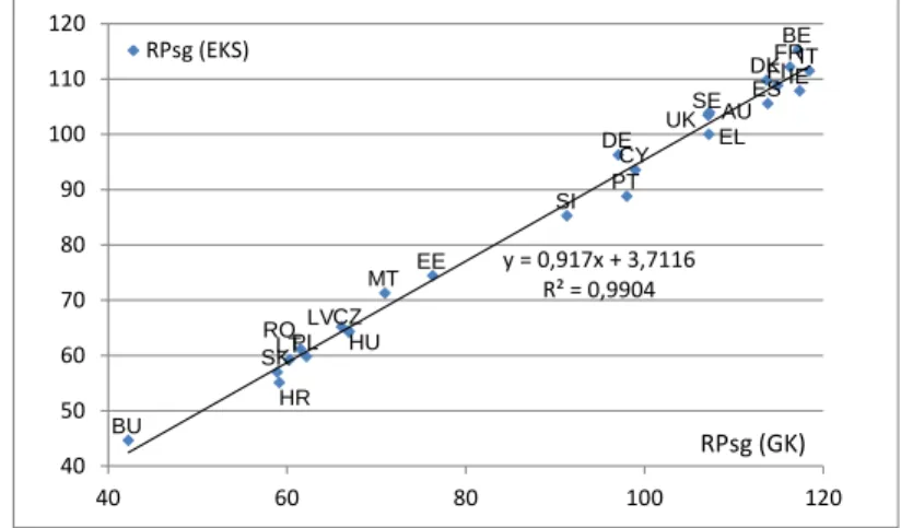
International data based on GK-PPPs used to be published by the OECD as supplementary information, but only for every third year (for the so-called “benchmark years” of PPP-based comparisons), and 2008 is the last year for which this type of information is available. This implies that the data published by the Eurostat on an annual basis allows us only an approximate reconstruction of the “actual” relationship between PLgdp and its weighted components. It also implies that the relative price of services to goods (RPsg), as calculated from the annual Eurostat- data (based on EKS-aggregation), is an approximation of the “true” relative price of the two items (which would correspond to a relative price based on GK-aggregation).
To check whether or not the aggregation method has a considerable effect on the size of RPsg, we compared the two ratios for 2008, the last year for which both are available (Figure 4).
22 See the methodological manual on PPPs for the respective details (Eurostat – OECD, 2012, pp. 235-247).