Geotechnics

F

K

B

, S

I

,

G ^EOTECHNICS

1

I. P

1. C

,

Soil

According to an engineering approach, soil is the upper covering layer of the Earth's crust, on or in which engineering facilities are built or installed. It is also used as material of earthworks and it has an impact on stability, durability and proper use of buildings.

Soils are three-phase systems: the main components are solid, liquid and gaseous phases.

Rates of soil-components

Water content shows the wetness of soils. Symbol: or .

Gravimetric water content is calculated as a ratio of the weight of water ( ) and the weight of solid particles ( ). It shows the weight percent of moisture compared to the mass of the solid phase of soil. The weight of water in a soil sample is determined by oven-drying at 105°C until reaching constant weight. At this temperature a strongly bounded water layer cannot evaporate from the soil sample.

As water content is a proportion of weights, its value is not affected by compaction of soils, thus it can be determined from disturbed soil samples. Water content values depend on surface phenomenon and surface stresses on soil particles.

The water content of sands is usually about 5% (the thickness of the water layer on the surface is small), that of clays is about 20-30%, while the water content of organic soils can be up to 100-300% in natural conditions.

Void ratio

Void ratio characterizes the compactness of soils. Symbol: or . It is defined as a (volumetric) ratio of the volume of void-space (fluids and air together) ( ), and the volume of solids ( ) (see Figure 1.1).

Figure 1.1: Interpretation of gravimetric and volumetric ratios of soils (Mecsi, 2009)

The value of the void ratio depends on volumetric changes of soils (the void ratio of loose soils is higher than that of dense soils), thus it can be determined only from undisturbed soil samples.

The void ratio of a dense sandy gravel soil is about 0.3, that of a loose sand is about 0.6, while the void ratio of clays (in natural conditions) varies between 0.5 and 1.0 and decreases with depth of the soil layers.

Porosity

Porosity is defined as a (volumetric) ratio of the volume of void-space (fluids and air together) ( ), and the total or bulk volume of material ( ), including the solid and void components (see Figure 1.1). Symbol: or .

The porosity of soils can vary widely. The porosity of loose soils can be about n=50%, while the porosity of compact soils is about n=30%. Porosity value depends on grain size distribution, and higher porosity follows smoother grain size distribution. When a soil sample consists of grains of various sizes, the smaller particles can be enclosed in the pores between larger grains. The porosity of granular soils mixed with clays can be smaller (n=20%) than the theoretical value.

The porosity of cohesive soils is usually higher, it can be n=50-70%.

Organic soils can have extremely loose structure. The porosity of fibrous peat can be as high as n=80-90%.

Porosity values are significantly affect by the past or present loads (e.g. geological preload) on soils.

Saturation

Saturation shows the rate of fluids and air in the void-space, and it is defined as a (volumetric) ratio of the volume of fluids ( ) and the volume of void-space ( ). Symbol: or .

or

Saturation can be determined only from undisturbed soil samples. The theoretical value of saturation can range from 0 to 1. The saturation of soils under groundwater level is S=1.0, saturation of sands above groundwater level is about S=0.2-0.4 , but clays above groundwater level can be almost saturated (S=0.8-0.9).

Two parameters from the four above can describe clearly the condition of soils, e.g. e and S, which means there is a connection between these parameters:

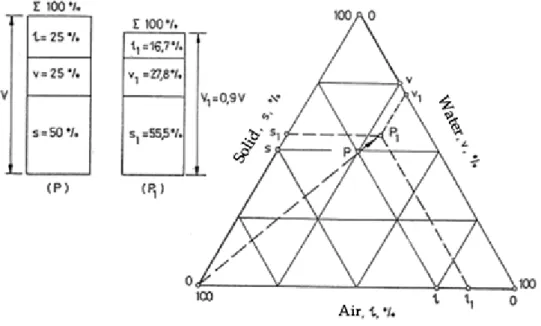
Volumetric rates of soil components

Volumetric rate of solids ( ) characterizes compactness, and is defined as a (volumetric) ratio of the volume of solids ( ), and the total or bulk volume of material ( ):

Volumetric rate of fluids ( ) characterizes soil moisture, and is defined as a (volumetric) ratio of the volume of fuids ( ), and the total or bulk volume of material ( ):

Volumetric rate of air ( ) is defined as a (volumetric) ratio of the volume of air ( ), and the total or bulk volume of material ( ):

Description of soil condition requires only two independent parameters; clearly, from these the third can be calculated:

Soil condition can be characterized by one point in a ternary diagram, as seen in Figure 1.2. Changes in soil condition can be illustrated as vectors connecting the characteristic points of different soil conditions.

Figure 1.2: Characterization of volumetric rates of soil components in ternary diagram

Density and bulk density

Density (particle density or bulk density) or is defined as the mass of particles of the

material ( ) divided by the total volume they occupy ( ):

The particle density or true density of a particulate solid or powder is the density of the particles that make up the powder, in contrast to the bulk density, which measures the average density of a large volume of the powder in a specific medium (usually air). The total volume includes particle volume, inter-particle void volume and internal pore volume.

The density of solid particles, water and air must be known for practical calculations. The solid part of soils consists of many different mineral particles, and their density can vary. Gravel and sand soils consist of mainly quartz grains, while clays consist of mineral particles of higher density.

Based on experience, we find that the particle density of solid granules of soils varies within narrow limits ( ), therefore average density values or values from tables of standards can be taken into account.

Natural (or wet) bulk density ( ) is defined as the full (wet) mass of particles of the material ( ) divided by the total volume they occupy ( ):

Typical values of natural density of soils vary within . This value is usually applied for calculations of soil mass (net weight, geostatic pressure, earth pressure).

Dry bulk density ( ) is defined as the dry (dried) mass of particles of the material ( ) divided by the total volume they occupy ( ):

It is used as a compactness indicator in earthwork construction.

Saturated bulk density ( ) is defined as the total mass of particles of the saturated soil material ( ) divided by the total volume they occupy ( ):

Underwater bulk density ( ) is a derived value for calculations of density of soils underwater:

, where is the density of water.

Consistency limits

The strength of connections between soil particles changes with water content in soils containing clay minerals.

Therefore, these soils behave differently with different water content depending on the (quantitative and qualitative) clay mineral content.

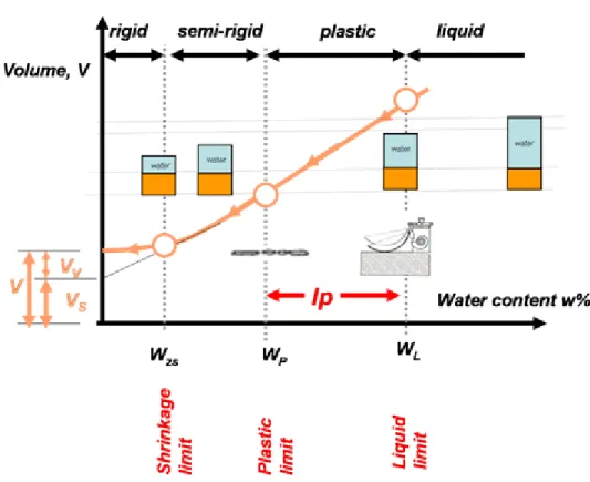
The original condition of soils changes in contact with water. Higher water content makes soils liquid, drying soils slowly leads to plastic consistency, reaching at the end the firm condition of constant volume. These transitions are continual.

Water contents where soils show specific properties are called consistency limits. For determination of consistency limits disturbed, kneaded soil samples are used. An interpretation of consistency limits is shown in Figure 1.3.

The determination of consistency limits is performed on saturated soil samples by equipment and methods described in international standards.

Figure 1.3: Interpretation of consistency limits (Mecsi, 2009)

Liquid limit

Liquid limit ( ) is the water content separating liquid and plastic condition. The practical meaning of liquid limit is that soils at the consistency of liquid limit slip down a slope of approximately 10°.

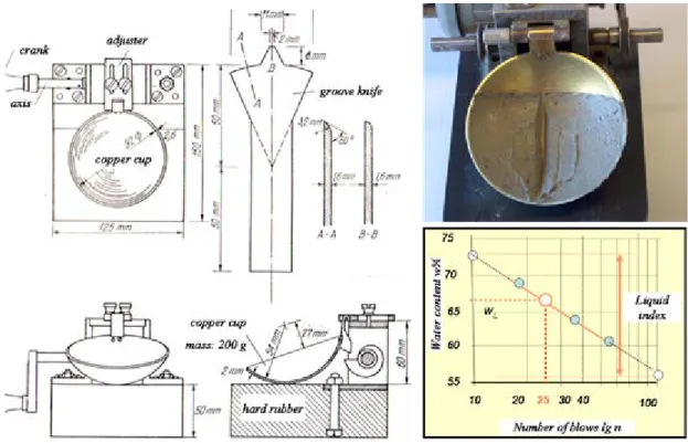
The liquid limit can be determined using the so-called Casagrande method – see Figure 1.4 and Video 1.1.

A groove is made with a standardized tool in the soil sample placed into the metal cup of this equipment and the cup is repeatedly dropped onto a hard rubber base, during which the groove closes up gradually as a result of the impact.

The number of blows for the groove to close for 10 mm is recorded, and the water content of the soil is determined.

The test must be repeated at higher water content (by adding water to the soil sample). A relationship between the number of blows and water contents can be graphed, and the liquid limit can be read from this graph. The moisture content at which it takes 25 drops of the cup to cause the groove to close is defined as the liquid limit.

This value of water content is considered as liquid limit – very typical of soil types and of connections between soil particles and water - and it varies usually between 35% and 100%.

The physical background of determination of liquid limit is looking for the moisture content at which soils show definite deformation against certain impact.

Experience shows that the number of blows–water content curves (the so-called liquid lines) of soils of different plasticity are parallel lines drawn in a semilogarithmic coordinate system.

Figure 1.4: Determination of liquid limit using Casagrande equipment

VIDEO 1.1

Video 1.1: Determination of liquid limit using Casagrande equipment

New European standards recommend another method: the so-called cone penetrometer test (Figure 1.5). It is based on the measurement of penetration into the pulpy soil of a standardized cone of specific mass in 5 seconds time.

Liquid limit is the water content where this penetration is equal to 10 or 20 mm. It can be determined by the graphing method already known from Casagrande method. Practical experiences show that cone penetrometer tests give more accurate results for low plasticity soils. An additional advantage is that the liquid limit can be theoretically determined based on one point (one test)

Plastic limit

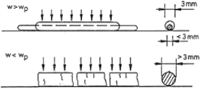
Plastic limit ( ) is the water content at which soil starts to transform from plastic to rigid condition, in other words from kneadable to brittle. The plastic limit is defined as the water content of soil when the soil sample can be rolled to a diameter of 3 mm and it just begins to crumble.

Determination of the plastic limit is based on this definition: we try to roll the soil sample to a thread of 3 mm. If the sample is about to break up, the water content of the soil sample is exactly on the plastic limit (Figure 1.6, Video 1.2), so the plastic limit can be determined by the calculation of the water (moisture) content of this thread.

Figure 1.6: Determination of plastic limit

VIDEO 1.2

Video 1.2: Determination of plastic limit

The plastic limit is of great importance in engineering aspects. Performing soil tillage or earthworks is the most economical and the simplest in this condition, when both manual and mechanical grading require the least amount of power. Dirt roads are passable, and embankments can be most easily compacted (reaching the smallest possible void ratio) when the water content of the soil is at its plastic limit.

Plasticity index

The plasticity index ( ) is the difference between the water content of the liquid limit and the plastic limit.

A small plasticity index refers to water-sensitive soils while a higher value means higher water absorbent capacity, and thus the quantity and quality of clay minerals can be characterized indirectly.

The plasticity index is also a measure of the cohesion ability of soils. A higher plasticity index usually means a higher expected value of cohesion (by the same compactness).

The plasticity index has an important role both in soil classification and in empirical formulas.

Experience obtained during determination of the value of plasticity index result in several empirical correlations.

Shrinkage limit

When drying a liquid or plastic soil mass, reduction of volume occurs to the same extent as water leaves. Shrinkage is caused by the capillary forces acting on the surface of the soil clod. At a certain water content these forces can not cause further volume reduction, volume ceases to change, the saturated soil becomes slowly unsaturated, and air phase substitutes moisture phase in the pores (see Figure 1.3).

The water content where further loss of moisture will not result in any more volume reduction is called the shrinkage limit ( ) or ( ).

The finer-grained soil and the higher content of clay minerals results in the higher value of shrinkage. The quality of clay mineral content (Na-montmorillonite vs. Ca-montmorillonite), the lattice structure of clay minerals, and the thickness of the diffuse double layer are particularly important to the measure of shrinkage.

Activity

As above, consistency limits are highly influenced by clay mineral content. Soils with the same clay content can show different behaviour, thus we have to distinguish between clay content and clay mineral content. Clay content is the rate of the particles smaller than 0.002 mm ( ), while clay mineral content is the quantity of clay minerals in the soil sample. Determination of the clay mineral content of a soil sample is not enough to draw conclusions about the behaviour of the soil, because there is a difference in its behaviour depending on the principal clay mineral (e.g. montmorillonite, illite, kaolinite). This property is particularly important in environmental protection for the determination of water and contamination retention capability. Skempton’s Activity value ( ), is especially useful for evaluating this behaviour. Skempton’s Activity is not a consistency parameter, but affects the values of consistency limits.

The value of activity can be calculated from the plasticity index ( ) and :

Skempton’s Activity value of the most important clay minerals:

Kaolinite: ;

Illite: ;

Montmorillonite: .

2. P

Characterization of particles is based on their size. Grain size can be typified by nominal diameter. The aperture of screens (rounded) or sieves (square) that lets a particle through identifies the nominal diameter. The nominal diameter of smaller particles is defined as the diameter of a ball of the same material as the particle with the same sedimentation speed in a liquid. The widely varying range of nominal diameter is divided into fractions.

The particle fraction names of Figure 1.8 can be used based on the new European Standard of soil classification. (The former Hungarian Standard named the particle fraction between 0.1 and 0.02 mm-s sandflour.) The abbreviations of fraction names originate from the first letters of English fraction names.

Soils of natural origin consist of a variety of particle sizes, or even several fractions. Thus, the size of particles can be characterized by grain size distribution showing the probability of occurrence of particle sizes. The grain size distribution is determined by sieve analysis and/or elutriation (sedimentation technique) (Figure 1.7-1.8). In the course of sieve analysis – according to the definition of nominal diameter – the mass rate of particles falling through sieves of different apertures is determined.

In geotechnical practice particle size analysis of fine particles is determined by elutriation, where density of the aqueous suspension of the soil sample is measured, and shows the settling velocity of particles. Stokes’ Law says that settling velocity is proportional to the square of the spherical particle diameter.

The density of the soil-liquid suspension is proportional to the proportion of the particles not settled. By measuring density during sedimentation, related nominal diameters and mass rates can be determined. Stokes’ Law is applicable

only for spherical particles; real grain size distribution can be derived by correction.

Figure 1.7: Sieve analysis and elutriation (Mecsi, 2009)

Figure 1.8: Determination of grain size distribution, typical grain sizes, derived parameters (Mecsi, 2009)

In earth sciences there are other methods for the determination of grain size distribution. Grain size is calculated based on Stokes’ Law, but the amount of particles falling out from a certain fraction is measured directly (Köhn pipette method, decantation).

The most expressive way of illustrating grain size distribution is by drawing a graph that which shows the proportion of

the mass of particles smaller than a certain diameter compared to the full particle cluster mass. Since particle size varies widely, it is shown in logarithmic scale.

The bounding of soil types and limits of particle fractions are more or less arbitrarily established, but the new European Standard determines the particle fraction limits differently than the former Hungarian Standard does.

The former Hungarian Standard used to name a particle fraction "sandflour", while the European Standard ranks this fraction partly as fine sand, but largely as silt. Hungarian geological practice names the fraction between 0.06-0.002 mm-s "rock flour".

Particle fraction limits according to new European Standards are shown in Figure 1.9.

Figure 1.9: Particle fraction limits and names according to new MSZ EN (Hungarian Standards introducing European Standards) and former MSZ (Hungarian Standard) (Mecsi, 2009)

Particle size distribution is often given by only the proportion of each fraction.

There are also several numerical parameters to characterize grain size distribution. The most important parameter is the inequality coefficient, calculated by the formula (formerly denoted by U). This characterizes the continuity of the grain size distribution and gives information about the compactability of soils. A soil of one particle size with about is difficult to compact, in contrast to a mixed soil with higher values.

The parameters of and (the so-called significant particle size) play an important role also in the characterization of some kind of sands, which show liquefaction (quicksand) under certain adverse circumstances (flow pressure, increasing neutral stress, earthquake, etc.). This is especially characteristic of nearly spherical particles,

with and .

The effective particle size ( ) is used for characterizing the water-related behaviour of the particles. It is defined as the diameter of the sphere with equal specific (based on mass unit) surface to the examined soil sample. For approximation can be used.

Some typical particle size distribution (PSD) graphs are shown in Figure 1.10 (from Szepesházi, 2008). The "A" curve belongs to silty sand, consisting of particles of almost the same diameter (so-called quicksand), The "B" curve is a good example of a continous particle size distribution (mixed or well-graded soil), and the "C" curve shows the (stepped) PSD of a fraction-deficient sandy gravel.

3. S

The main goal of soil classification is to obtain the most important properties of a tested soil sample, right after classification, using experience collected about each group. To reach this goal, soil classification must be based on these most important and most typical properties and parameters. The new soil classification system (realized in 2006 and based on the new European Standards of soil classification) will be introduced next. Old soil classification methods will also be mentioned briefly.

Naming and indentification of soils

The naming of soils refers to and is based on the particle composition and the importance of the particle-water relations. The name of soils is their fixed parameter, which can change only because of specific influences (e.g. great forces causing particle beaking, or weathering because of the chemical environment).

Granular soils are named based on their particle size distribution, because their behaviour is determined by particle composition. Cohesive soils are classified based on their plasticity index, as their behaviour is determined mainly by particle-water relations.

Soil names must be determined based on the new MSZ 14043-2 Hungarian Standard as follows:

Based on particle size distribution, if and ;

Based on plasticity index, if and ;

Based on classification of adjacent layers and geological origin, if criteria on both particle size distribution ( ) and on plasticity index ( ) lead to a contradiction.

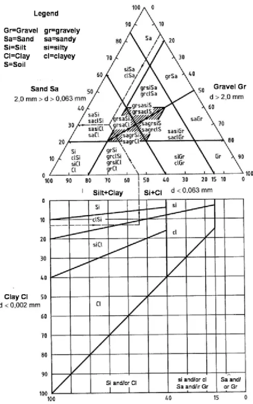
Soils must be named based on particle size distribution as shown in Figure 1.11. The parameters of soils (depicted on the axes of this ternary diagram) must be determined and plotted, and these parameters mark one point - characteristic of the soil. The soil is named from the region of the ternary diagram where this characteristic point lies.

The lower part of the ternary diagram helps to separate silt and clay fractions, and silty or clayey attributives can be chosen.

(The soil example shown in this figure should be named silty clay based on this diagram, but these kinds of soils must be named based on plasticity index.)

Figure 1.11: Classification of granular soils based on MSZ 14043 -2

The larger fraction gives the name of granular soils according to former Hungarian soil classification. The following fraction(s) (containing "enough" of it) gave the attributive. The sufficient amount was 20% for gravel, sand, and sandflour, and 10% for silt and clay.

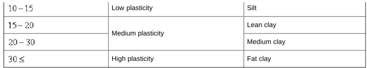
Classification of cohesive soils is based on the plasticity index, see Table 1.1.

The European Standards recommend the attributives shown in the middle column, but allow fixing the limits in the first column for every nation. The additional Hungarian Standard made this change, and attached the old (Hungarian) names to these new limits.

Plasticity index Group name based on MSZ EN ISO

14688-2:2005 Name based on MSZ 14043-2:2006

Non-plastic Based on particle size distribution

Low plasticity Silt

Medium plasticity

Lean clay Medium clay

High plasticity Fat clay

Table 1.1.: Classification of cohesive soils

Organic nature must appear in the appellation of soils. Soils with an organic content between are slightly organic, between are moderately organic, and above are highly organic. Classification was more rigorous before: cohesive soils with an organic content above 5% and granular soils with an organic compound above 3% were called organic.

The new European-Hungarian Standard categorizes organic soils separately and classifies them based on appearance and components (different kinds of peats, marsh sediments, humus).

Colours of soils must be also mentioned, because this helps soil identification on site and gives other information.

Besides, it could be of service to refer to geological origin and characteristics, and to all other important properties, e.g. artificial origin, possible pollution, local names, etc.

4. D

Soils can be classified into two main goups based on the origin of shear strength: cohesive and cohesionless soils.

Between the particles of cohesive soils there are inner cohesive forces, while the shear strength of cohesionless soils is due to the friction between particles and their clinging to each other.

While friction strength is interpreted only in presence of normal forces, there is no shear strength of cohesionless soils if the normal load is zero. By contrast, the cohesion of cohesive soils is the shear strength at zero normal load.

It is very important to emphasize that the basic rule is that the shear strength of granular soils originates only due to effective stress, in other words this shear strength is mobilized only by effective normal stress.

In cohesionless granular soils , thus shear strength can be characterized by the inner friction angle. Slightly wet, partially saturated granular soils have some cohesion, too. This is created by the capillary effect of pore water, and ceases if soils become saturated or dry. Therefore this is called pseudo (apparent) cohesion and is ignored in calculations.

Shear tests

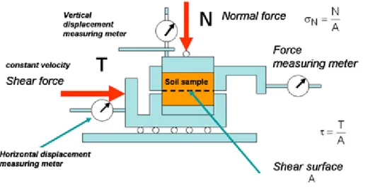
Shear tests are performed by constant normal stress, increasing shear stress until soil sample failure. In geotechnical practice, the most frequent method is the so-called direct shear, when the shear test is performed in a shear box, made of two half boxes moving away from each other (Figure 1.12 and Video 1.3).

Figure 1.12: Principles of direct shear (Mecsi, 2009)

VIDEO 1.3

Video 1.3: Direct shear

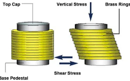
In reality failures similar to direct shear are rare, but there are shear tests closer to the so-called pure shear. Pure shear is difficult to realize by simple experimental techniques, but there are equipment in geotechnical practice based on the principle of simple shear, where the smaller side wall effect results in more homogenic stress and deformation fields compared to direct shear equipment. Principles of simple shear are shown in Figure 1.13.

Figure 1.13: Principles of simple shear

As mobilized shear strength is a function of shear displacement, in certain cases the so-called residual shear strength must be determined as well (e.g. surface movements, soil-geosynthetics slip on each other). Residual shear strength can be determined using torsion shear equipment. Principles of torsion shear (or simply torsion) are shown in Figure 1.14.

Figure 1.14: Principles of torsion shear

Processing of test results

Stresses are calculated by dividing the applied normal and shear forces with the surface of the sheared cross-sections:

Curves of correlation between shear stresses and strains are depicted for all normal loads (Figure 1.15). From these curves we can read:

a) the proportional limit, namely the value of stress until displacements are proportional to shear stress;

b) the maximum shear stress;

c) and, if different from the maximum, the residual value of shear stress.

The Mohr-Coulomb failure lines can be drawn by depicting these values as a function of the applied normal stress.

The incline of these lines gives:

a) the "proportional" friction angle;

b) the maximum of friction angle;

c) the residual value of friction angle (belonging to permanent slide).

Figure 1.15: Processing of direct shear test results

Shear test results of compact and loose sands are shown in Figure 1.16.

Figure 1.16: Results of shear tests of compact and loose sands

From direct shear tests, failure surface on the constraint surface between the two half boxes was only a hypothesis.

Surfaces shown in Figure 1.17 and Animation 1.1 were proven by experience.

Figure 1.17: Shape of failure surfaces during direct shear

ANIMATION

Animation 1.1: Shape of failure surfaces during direct shear

Uniaxial compressive strength

This method is suitable only for the determination of the strength of cohesive soils. A cylindrical soil sample is loaded in axial direction between two compression plates, gradually increasing the load until failure. The vertical ( ) and the horizontal ( ) deformation of the sample is measured during loading. The method of load transfer can be fast or slow, continous or discontinous (step).

The results of the test are shown in Figure 1.18. The residual deformation after unloading is greater than the elastic deformation.

Most soils show this behaviour. The elasticity modulus calculated in this figure is not specific for soils, thus cannot be used for calculations of the deformation.

The compressive strength obtained as a final result from the test is only a comparative value between the same types of soils.

Figure 1.18: Results of the uniaxial compressive strength test

Triaxial compression test

A cylindrical soil sample in a compression cell is loaded by hydrostatic pressure first, than loaded by vertical pressure until failure during the triaxial test.

The Mohr circle of the tension condition resulting in failure is drawn, and the test is performed repeatedly at different hydrostatic pressures. The cohesion and the inner friction angle of the soil can be read from the envelope of the Mohr circles of failure, the so-called Coulomb failure line.

The apparatus used for triaxial tests is shown in Figure 1.19 and Video 1.4. The main parts of the apparatus are the cylinder (made of glass or transparent plastic) and the well-sealed base and cover plates. The soil sample, surrounded by rubber, is placed in the liquid-filled (usually water-filled) space on the base plate sealed with rubber rings. There are filters below and above the sample, connected to capillaries.

These capillaries communicate through the bores of the base plate with the volume change measuring device and the pore water pressure measuring device.

The vertical load is transferred by the piston pressing on the top cap, and the loading force is measured. The measured

displacement of the piston shows the vertical displacement of the sample. The side pressure can be controlled by a pressure regulator.

Figre 1.19: The tiaxial test and the processing of the results of the measurements

VIDEO 1.4

Video 1.4: The tiaxial test

Animation 1.2: The triaxial test (SOIL MECHANICS, A. Verruijt, TU Delft, 2001)

The drainage of water (assuming saturated condition) from the soil sample can be controlled by the shut-off and opening of a tap on the tube. The system can be closed or opened. This depends on the allowance of the consolidation of the sample or the development of the pore water pressure inside the sample. The test can be performed in three different ways:

a) Unconsolidated fast test (Unconsolidated Undrained (UU)): In an unconsolidated undrained test the sample is not allowed to drain. The sample is compressed at a constant rate (hydrostatic pressure) with the tap closed. The vertical stress is increased with the tap closed as well. The speed of compression is steady, 0.5-1.0% of the height of the sample per minute. The pore water pressure is measured during this test.

b) Consolidated fast test (Consolidated Undrained (CU)): In a consolidated undrained test the sample is not allowed to drain. The consolidation of the sample under hydrostatical pressure (with the tap opened) must take place before increasing the vertical stresses, than the vertical pressure is increased until failure with the tap closed. The pore water pressure is measured during this part of the test.

c) Slow (consolidated) test (Consolidated Drained (CD)): the full consolidation under hydrostatical pressure the vertical load is increased gradually, and the consolidation of the sample is allowed to take place in every load step.

During both the hydrostatical and the vertical load steps the pore water pressure is measured. The consolidation can be considered completed when the pore water pressure measuring device shows zero. This usually takes a long time, thus test can be run for days.

Tests of unsaturated samples can be performed without the measurement of the pore water pressure. In this case, the results of the tests can be graphed only as a function of the total stresses. The result of this is also the apparent friction angle.

Figure 1.20 shows the determination of the shear strength as a function of the total and the effective stresses.

Figure 1.20: The determination of the Coulomb failure line as a function of the total and the effective stresses

ANIMATION

Animation 1.3: Drained triaxial test (SOIL MECHANICS, A. Verruijt, TU Delft, 2001)

ANIMATION

Animation 1.4: Undrained triaxial test (SOIL MECHANICS, A. Verruijt, TU Delft, 2001)

Knowing the value of total stress and pore water pressure (both measured during the test) the Mohr circles of the effective principal stresses and the Coulomb failure line can be drawn as a function of the effective stresses. It is obvious that the diameter of the Mohr circle of the principal stresses is the same in the two cases, but their location is different, so it follows that the shear strength parameters determined as a function of the total and the effective stresses will not be the same ( ; ), and thus the Coulomb failure line will be a function of the method of the test (UU, CU or CD).

Triaxial cells can be used – besides for shear strength tests - to determine the hydraulic conductivity of low permeability soils in environmental geotechnics. The main advantage of these tests is the possibility of preventing the side wall leakage, which is the main source of error in the determination of the hydraulic conductivity of low permeability soils (e.g. clays, liner layers). Figure 1.21 shows the determination of the hydraulic conductivitiy of a clay sample.

Figure 1.21: The determination of the hydraulic conductivity of clays in a triaxial cell

Problems of shear strength tests of soils

The shear strength of granular soils is a relatively simple problem. Granular soils behave almost always as "open systems" (depending on the shear speed) and their failure can be examined by the analysis of the effective stresses.

Their inner friction angle is and depends on the:

Grain size: of gravels, and of sands is typical;

The continuity of grain size distribution: can change by depending on the (inequality coefficient);

The compactness: the difference between the of the loosest and the most compact soils can be ;

The roughness of the surface of the soil particles: this can result in about difference in .

The shear strength of dense sands can decrease because of the dilatation after the large shear deformations and can fall back to the residual value (see also Figure 1.16). The decrease of the inner friction angle can be characterized by the dilatation angle, which can be as much as .

The cohesion of granular soils is zero both in saturated and in dry condition, but in unsaturated condition they can have a cohesion of because of the capillary effect. This cohesion can be ignored by calculations, because saturation or drying-up eliminates it.

The shear strength of cohesive soils is a more difficult problem. The test results are affected by several factors:

They behave as an opened or closed system depending on the speed of load;

The shear strength depends on the load speed because of the viscous properties;

They tend to creep because of the same reason, and the creeping can lead to failure;

The preload can increase shear resistance;

The strength of preloaded clays can decrease, as well as the strength of compact sands.

The literature gives many measurement results, and there are empirical functions to describe certain effects (Szepesházi, 2008).

5. T

The load-induced deformation of soils can be determined by several laboratory methods, but the application of some side support is usually needed. The soil can be considered as an infinite halfspace by foundations. Thus the deformations in side directions are inhibited. In laboratories this condition can be best generated in triaxial cells, but the so-called oedometric tests with inhibited side deformations (Figure 1.22) are the most widely used methods because of their simplicity. In this case the side deformations are prevented and the soil is loaded in a closed ring. This is the stress condition of compression.

The soil sample is placed in a steel ring. Its diameter is , its height is , (a rate is needed). Through the porous filter under and above the soil sample, the water (forced out of the sample because of the compression) can be drained.The deformation of the sample can be only vertical because of the rigid bin of the ring. The load is applied in the centre of the load distribution plate placed above the upper filter stone. The usual load steps are the following during these tests: , but offloading and re-loading can be applied also. During the test the vertical deformation of the sample ( ) is measured, the temporal evolution of the deformations and the specific deformations are determined:

The load is applied gradually. Each load step needs more time to transform neutral stresses into effective stresses. A load step runs until the sample becomes consolidated. For tests of clays this usually takes 5-24 hours.

Figure 1.22: Cross section of the oedometer

Signs: 2 filter; 3 load distribution plate; 4 and 9 sample holder rings; 5 bottom plate; 6 -7 -8 sealing plate, clamp ring, screws; 10: pipe for water inlet and outlet

The processing of the results gives the compression curve (Figure 1.23). The compression curve can be described by a power function for the majority of soils. This processing is advantageous for computer calculations, since the hardening-up properties of the soils can be well characterized.

The compression modulus of soils can be defined as the stress by unit specific compression, thus it is a function of stress for compressive soils. The compression modulus of the soil is at .

Other deformation phenomena can be examined by oedometer tests:

Loess slump: the potential load of the soil is applied on the sample, than the sample is irrigated with water and the static and the sudden slump is measured and determined as specific compression.

Swelling of clays, the determination of the swelling pressure: The increase of the void ratio (swelling) is measured when applying real normal load, or the pressure which stops the swelling entirely is determined.

The oedometer can be used also for the determination of the hydraulic conductivity of soils. In this case, water pressure is applied to the sample through the tube marked 10 in Figure 1.22 and the water quantity leaking through the sample is measured by constant water pressure, or the pressure drop is measured by variable pressure. This method is applicable primarily to low permeability soils. An advantage is the possibility of the determination of the change of the hydraulic condutcitivity as a function of the compactness of the soil (performing the test gradually at different load steps).

Figure 1.23: Processing of the results of the compression test (Mecsi, 2009)

6. T

The compressibility of soils can be determined performing the so-called Proctor test. Two tests (with different specific compression work) are applied usually (Figure 1.24 and Video 1.5). Hungarian practice used the standard test earlier but more recently, uses the modified Proctor test.

VIDEO 1.5

Video 1.5: The Proctor test

Performing the modified Proctor test, the prepared soil sample with constant water content is compacted into a standard ( ) pot applying standard compression work in 5 equal layers. After compaction the wet density ( ), the water content ( ) and the dry density ( ) of the sample are determined. This action is repeated at least 5 or 6 times by increasing water contents and the results of the tests are graphed as seen in Figure 1.25, resulting in the so-called Proctor curve. The results are "good" if the values of the wet and dry densities form a concave curve as a function of the water content. The "top" of the curve is the maximum dry density ( ) determined by the Proctor test.

Figure 1.24: The Proctor test and the processing of the results

Figure 1.25: The Proctor curve

This method is suitable for the examination of both coarse and fine-grained soils (gravel, sand, silt, clay).

The compressibility of soils depends on the size, the shape of the particles, the quality of their surface, the value of the water content, the rate of compression work, the method of compaction, physical and chemical effects, etc.

It is very important in environmental aspects (by the building in of liner layers) that the compacted soil structure on the dry side ( ) is different from the soil structure on the wet side ( ), and this phenomenon affects the sealing capacity of the built liner layer. The optimal lining capacity can be achieved at the wet side, by water contents

larger than the optimal water content (Figure 1.26).

Figure 1.26: The affect of the compaction method and the water content during installation on the hydraulic conductivity of clays (Mitchell et al., 1965)

7. T

Granular soils

The density of granular soils is a very important property, thus this must be determined. The new Hungarian Standard defines the density index with this correlation:

, namely the actual void ratio must be compared to the void ratio (typical of the loosest condition of the examined soil) and the void ratio (typical of the most dense condition of the examined soil). The soil condition can be classified based on this value according to the Table 1.2.

The previous Hungarian Standard contained this term, but it was named relative compactness, denoted by , and three different categories were given named (loose–medium compact–compact).

The classification of the compactness of granular soils

Name Compactness index

Very loose 0–15

Loose 15–35

Moderately dense 35–65

Dense 65–85

Very dense 85–100

Table 1.2: The classification of the compactness of granular soils

Cohesive soils

The condition of cohesive soils depends on their water content, thus consistency must be classified. This is (was) based on the following formula of relative consistency index in both the previous and the new European and Hungarian Standards:

The new standard gives the attributives as seen in Figure 1.27.

Figure 1.27: The interpretation of the consistency index and the names of the conditions of cohesive soils

Digitális Egyetem, Copyright © Faur Krisztina Beáta, Szabó Imre, 2011