Hierarchical steering control for a front wheel drive automated car

Hierarchical steering control for a front wheel drive automated car

S´andor Beregi^∗, D´enes Tak´acs^∗∗, Chaozhe R. He^∗∗∗, Sergei S. Avedisov^∗∗∗, and G´abor Orosz^∗∗∗

∗Department of Applied Mechanics, Budapest University of Technology and Economics, Budapest, Hungary (e-mail: beregi@mm.bme.hu)

∗∗MTA-BME Research Group on Dynamics of Machines and Vehicles, Budapest, Hungary (e-mail: takacs@mm.bme.hu)

∗∗∗Department of Mechanical Engineering, University of Michigan, Ann Arbor MI, USA (e-mail: hchaozhe@umich.edu,

avediska@umich.edu, orosz@umich.edu)

Abstract:

In this study the lateral control of an automated vehicle is analysed with the help of a single- track model while subject to a hierarchical control algorithm. At the higher-level we command the steering angle based on the vehicle’s relative position and orientation to the desired path, while the lower-level controller tries to achieve this angle by adjusting the steering torque. The stability of the straight-line motion is investigated by incorporating time delays at both control levels. We demonstrate that the two control algorithms can be designed independently from each other. Moreover, we show that the stability of the lower-level controller is highly sensitive to the delay, that is, to ensure stability very high sampling frequency is required.

Keywords:automotive control, vehicle lateral control, steering control, linear stability 1. INTRODUCTION

In recent years automated driving of cars and different computer-based driving aid systems became increasingly well-spread. One essential task demanded from these con- trol algorithms is to follow a given path with given speed (Falcone et al., 2007),(Kayacan et al., 2016). It is common to deal with this problem using two separate controllers assigned to the longitudinal and the lateral dynamics of the vehicle (Ulsoy et al., 2012). Our analysis here focuses on the lateral control. One of the simplest case is to follow a straight line with the vehicle, e.g., a lane on the highway.

This simple manoeuvre can be used for selecting the gains of the lateral control algorithm as such experiments can be conveniently conducted on test tracks.

As in every control algorithm, time delay influences the stability of steering controllers as shown in (Shuai et al., 2014),(Jalali et al., 2017). In this paper we consider a hier- archical controller. The higher-level controller determines the desired steering angle based on the vehicle’s position and orientation with respect to its desired path, while the lower-level controller determines the corresponding steer- ing torque needed. Consequently, two different time delays appear in the system corresponding to the two different control loops. The delay in the higher-level is of magnitude 0.1-0.3 s. This is related to the time needed for processing camera images and GPS signals. The lower level controller may also contain delay up to a few milliseconds and this is related to the sampling frequency of that controller. In the present study we focus on the analysis of the straight-line motion with specific attention on how and to what extent the two delays influence stability.

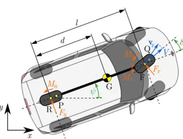
Fig. 1. The in-plane, single-track (so-called bicycle) model of a front wheel drive car.

2. VEHICLE DYNAMICS AND CONTROL DESIGN To describe the lateral and yaw motion of the car we utilize an in-plane single-track model shown in Figure 1 which is widely used to study vehicle handling (Pacejka, 2012). The position and orientation of the vehicle in the horizontal plane are given by the componentsxandy of the position vector of the center of gravity G and the yaw angle ψ.

The front axle of the vehicle is steered as represented by the steering angle δ. These four generalized coordinates describe the configuration of the system unambiguously.

The geometry of the vehicle is described by the wheelbase l and the distance of the center of gravity from the rear axle denoted by d. Moreover, the mass of the vehicle is denoted bymwhile its moment of inertia about its center of mass is denoted byJG. The mass of the steering system (including the front wheel) is denoted by mF while the moment of inertia about the center of the front wheel F is denoted byJF. (The mass and the mass moment of inertia of the rear wheel are incorporated inmand JG.)

We distinguish between the specific points of the wheels and tire-ground contact patches. In Figure 1, F and R denote the wheel centers for the front and rear tires, respectively. The leading points, where the center lines of the treads enter the contact regions are referred by Q and P, respectively. In order to eliminate the longitudinal dynamics we neglect the longitudinal deformation of the tires and consider that the driven wheels rotate with constant speed. Since we consider a front wheel drive car, we prescribe the wheel directional component of the velocity of the wheel center F to be a constant V. This poses a nonholonomic constraint on the dynamics of the system.

To derive the equations of motion we use the Appell-Gibbs formalism (Gantmacher, 1975),(De Sapio, 2017) which requires the introduction of the so-called pseudo velocities.

Since the configuration is described by four generalized coordinates and there is one nonholonomic constraint, we need to choose three pseudo-velocities. Here we chooseσ1

to be the lateral velocity of the center of gravity G,σ2 to be the yaw rate of the vehicle whereas σ3 is the steering rate (the yaw rate of front axle relative to the car). The nonholonomic constraint and the definition of the pseudo- velocities can be summarized using the matrix equation







cos(ψ+δ) sin(ψ+δ) (l−d) sinδ 0

−sinψ cosψ 0 0

0 0 1 0

0 0 0 1















˙ x

˙ y ψ˙ δ˙









=





 V σ1

σ2

σ3





. (1) Solving this equation the time derivatives of the gener- alised coordinates can be expressed as

˙

x=Vcosψ cosδ −σ1

sin(ψ+δ)

cosδ −σ2(l−d) cosψtanδ,

˙

y=Vsinψ cosδ +σ1

cos(ψ+δ)

cosδ −σ2(l−d) sinψtanδ, ψ˙=σ2,

δ˙=σ3.

(2)

These kinematic equations give part of the governing equations, while the other part is comprised of the Appell- Gibbs equations:

"m11 m12 0 m21 m22 JF

0 JF JF

# "σ˙1

˙ σ2

˙ σ3

#

=

"f1

f2

f3

#

, (3)

where the elements of the generalised mass matrix are given by

m11= mF+m cos²δ , m12=m21= mF+msin²δ

cos²δ (l−d), m22=JF+JG+mF+msin²δ

cos²δ (l−d)², (4)

while the right hand side can be expressed as f1= FF

cosδ+FR

+ 1

cosδ

−(mF+m)V +mσ2(l−d) sinδ σ2

+(mF+m) sinδ cos³δ

Vsinδ−σ1−(l−d)σ2

σ3, f2=MF+MR+(l−d)FF

cosδ −dFR

−l−d cosδ

mFV +mσ1sinδ σ2

+(mF+m)(l−d) sinδ cos³δ

Vsinδ−σ1−(l−d)σ2

σ3, f3=MF+MS.

(5) Here MS denotes the steering torque while FF, FR and MF, MR are the lateral tire forces and aligning torques calculated from the tire model. In particular, for the brush tire model these can be expressed by the formulae

F(α) =

φ3tan³α+φ2tan²αsgnα+φ1tanα, 0≤|α|< αcrit,

µFzsgnα, αcrit<|α|,

(6)

and

M(α) =







µ4tan⁴αsgnα+µ3tan³α+µ2tan²αsgnα+µ1tanα, 0≤|α|< αcrit,

0, αcrit<|α|,

(7)

as function of the slide-slip angleα.

The slide slip angles can be calculated from vehicle kine- matics as

tanαF=−σ1+ (l−d)σ2+a(σ2+σ3)

V cosδ + tanδ, tanαR=− σ1−(d−a)σ2

cosδ V − σ1+ (l−d)σ2

sinδ,

(8)

for the front and the rear wheels, respectively. In the formulae above µ denotes the friction coefficient, Fz is the vertical load on the tire whileαcrit corresponds to the critical side-slip angle at which the whole contact patch starts to slide. Moreover, the constantsφiandµiare given in Appendix A and adenotes the half-length of the tire- ground contact patch (i.e., the distance between F and Q and the distance between R and P).

Fig. 2. Qualitative lateral tire force (left panel) and align- ing torque (right panel) characteristics.

Formulae (6) and (7) are visualized in Fig. 2. While these characteristics are piecewise-smooth continuous functions,

for linear stability analysis of the rectilinear motion it is sufficient to use the continuous linear parts for small α, that is,

F(α)≈φ1α= 2a²kα, (9) and

M(α)≈µ1α=−2

3a³kα, (10)

whereais the half-length of the tire-ground contact patch whilekis the lateral stiffness of the tire distributed along the contact length; see the definition ofφ1andµ1in (A.1) and (A.4) in Appendix A. The constant 2a²k in (10) is often referred as the cornering stiffness.

Here we construct a hierarchical controller in order to regulate the steering torque MS such that the vehicle follows a straight path. Without loss of generality we make the vehicle to run along the x axis, i.e., y(t) ≡ 0 and ψ(t)≡0. At the higher-level we calculate a desired steering angle from the vehicle position and orientation as

δdes(t) =−kψsin (ψ(t−τ1))−kyy(t−τ1), (11) where kψ and ky are proportional gains for the lateral position and the orientation angle while a time delay τ1

represent the time needed for sensing, computation, and actuation. Then the steering torque is determined by the PID controller

MS(t) =kp(δdes(t−τ2)−δ(t−τ2))

+kd( ˙δdes(t−τ2)−δ(t˙ −τ2)) +kiz(t−τ2), (12) where τ2 represent the time delay in the control loop and the integral term is considered trough the variable z defined by

˙

z(t) =δdes(t)−δ(t). (13) In our study we consider the gains of the lower-level controller in the form of

kp=pkp0, (14)

kd=pkd0, (15)

ki=pki0. (16)

The benefit of this formulation is that parameterpcan be used to represent the ‘strength’ of the lower-level controller for a fixed set of the gainskp0, kd0andki0. Note thatp= 0 corresponds to the case of no control on the front axle, while p → ∞with τ2 = 0 corresponds to the case when the steering angle could be directly set with appropriately chosen control gains.

3. LINEAR STABILITY ANALYSIS

The closed-loop dynamics of the vehicle is described by the equations (2,3,11,12,13) that can be written into the compact form

x(t) =˙ φ(x(t),x(t−τ2),x(t−τ1−τ2)), (17) where

x= [x y ψ δ σ1 σ2 σ3 z]^T, (18) contains the state variables. The rectilinear motion can be expressed as

x^∗(t) = [V t 0 0 0 0 0 0 0]^T. (19) Let us introduce the perturbations ˜x(t) =x(t)−x^∗(t) and linearize (17) about the the rectilinear motion to obtain

x(t) =˙˜ A0˜x(t) +A2˜x(t−τ2) +A12x(t˜ −τ1−τ2), (20) where the matrixes A0, A2, and A12 are defined in Appendix B.

Using the trial solution x(t) = ce^λt we can obtain the characteristic equation as

D(λ) = det

A0+A2e^−λτ2+A12e^{−λ(τ1+τ2)}

= 0, (21) which has infinitely many solutions for the characteristic roots λ. Notice that λ = 0 is always a solution corre- sponding to the ‘neutral’ directionx. After eliminating this trivial eigenvalue by defining ˜D(λ) = D(λ)/λ, ˜D(0) = 0 provides the stability boundaries for non-oscillatory stabil- ity loss whereas ˜D(iω) = 0 gives the stability boundaries for oscillatory stability loss. These bound the stable do- main in the parameter space where all eigenvalues have negative real part. When crossing a ˜D(0) = 0 boundary a real characteristic root moves to the right half complex plane, while when crossing the ˜D(iω) = 0 boundary a pair of complex conjugate roots crosses the imaginary axis from left to right (St´ep´an, 1989). In this case oscillations arise with angular frequency close toω.

In order to calculate the stability boundaries numerically we use semi-discretisation (Insperger and St´ep´an, 2013).

In particular, we utilize Chebysev polynomials and the Chebysev differentiation matrix to approximate the infi- nite dimensional spectrum of (20); see (Trefethen, 2000).

Using these techniques we draw stability charts in the plane of the control gains for different values of the delays.

0 2

0 0.2

0 2

0 0.2

0 2

0 0.2

0 2

0 0.2

= 0.25 s = 0.3 s

= 0.15 s = 0.2 s

Stable

Stable

Stable Stable

Unst. Unstable

Unstable

Unstable

p = 250 p = 500 p = 1000

p = 2000 p = 4000

ky[1/m]

k [1] k [1]

ky[1/m]

ky[1/m]

k [1] k [1]

ky[1/m]

1 1

1 1

p = 8000

(6) (7,8)

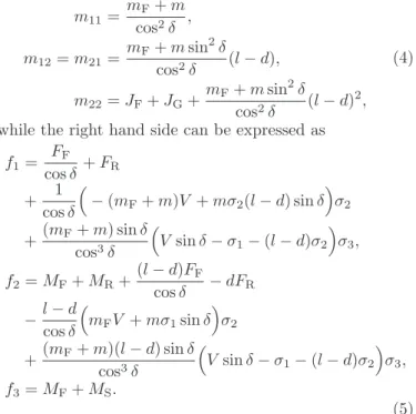
Fig. 3. Stability charts for different values of higher-level delayτ1 in the plane of the higher-level control gains kψ and ky with lower-level delayτ2 = 0.0001 s. The boundaries corresponding to different values of control strengthpare shown in different colours. On the left panels parts of stable regions are outside the window.

In Fig. 3 the stability boundaries are shown for different higher-level delays τ1 in the plane of the higher-level control gains (kψ, ky) corresponding to the lateral position and orientation of the vehicle. The different curves in each panel correspond to different values of parameterpwhile

2 2

2 2

0 1.5

0 0.15

0 1.5

0 0.15

0 1.5

0 0.15

0 1.5

0 0.15

= 0.93364235 ms = 0.93364241 ms

= 0.93364247 ms = 0.93364253 ms

ky[1/m] ky[1/m]

ky[1/m] ky[1/m]

k [1] k [1]

k [1] k [1]

Stable Unstable

Stable Unstable

Unstable Stable

Unstable

S.

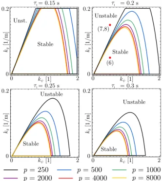
Fig. 4. Stability charts for different values of lower-level delayτ2in the plane of the higher-level control gains kψ and ky with higher-level delay of τ1 = 0.2 s and control strength ofp= 4000 are considered.

Unstable

Stable 0

0.006

10⁵

0 p [1]

2 [s]

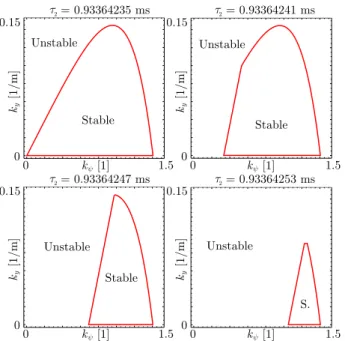
Fig. 5. Stability chart in the plane of the control strengthp and the time delayτ2of the lower-level controller. The higher lever gains are set to kψ = 0.5 and ky = 0.01 1/m whereas the higher-level delay of τ1 = 0.2 s is considered.

the lower-level delay is set toτ2= 0.0001 s which is small enough not to endanger stability. Then the lower-level control gains are set tokp0= 8 Nm, kd0= 0.1 Nms, ki0= 0.5 Nm/s while the vehicle and tire parameters are listed in Table 1 and they are kept the same in the rest of the paper.

It can be seen, that the size of the stable parameter domain strongly depends on the time delay in the higher-level control loop, i.e., the larger the delay is, the smaller the stable parameter domain is. The larger values of parameter presult smaller stable domains. However, this shrink has a lower limit corresponding top→ ∞.

If the delayτ2of the lower-level controller is non-zero but sufficiently small it has a negligible effect on the stability boundaries. However, within a very narrow interval of this delay the whole stable parameter region disappears, as shown in Fig. 4 where the lower-level delay is varied only by a fraction of a millisecond. This means that the critical value of the lower-level delay only very weakly depends on the parameters of the higher-level controller. Thus, the two controllers can be designed and investigated separately. In

the meantime, it can be established that the critical lower- level delay strongly depends on the control strength pas shown in Fig. 5.

The investigation of the imaginary parts of the critical eigenvalue reveals that the frequency corresponding to the arising vibrations are considerably different in the two control levels. If the higher-level control gains are chosen from the unstable parameter domain vibrations with a frequency up to∼3-5 Hz can be observed. On the contrary due to instabilities of the lower-level controller one can observe high-frequency vibrations (∼100-150 Hz).

4. SIMULATIONS 4

-40 20

y [m]

t [s]

0.2

-0.2

0 20

des [rad]

t [s]

Fig. 6. Time profiles for the centre of gravity’s lateral position (upper panel) and the desired (thick red) and actual (thin black) steering angles (lower panel) for control parameterskψ= 0.5,ky = 0.05 1/m,p= 4000 and time-delaysτ1= 0.2 s,τ2= 0.0001 s.

Numerical simulations have been carried out for the non- linear system to demonstrate the behavior for different scenarios. In Figure 6 the lateral position of the vehicle’s centre of gravity and the desired and actual steering angles are presented for a stable set of control parameters shown in the bottom left panel of Fig. 3. In Figures 7 and 8 we demonstrate the developing oscillations due to ‘badly’

chosen higher-level control gains. The two different initial conditions are applied to show that the system converges to a stable limit cycle. In Figure 9 we present the system behavior in the case when the delay in the lower-level controller is 1 ms that is larger than the critical value.

5. CONCLUSIONS

In this paper a hierarchical lateral controller of an au- tonomous vehicle was investigated considering different

Table 1. Vehicle and tire parameters

Parameter name Value Unit

l wheelbase 2.57 m

d center of gravity position 1.54 m

m vehicle mass 1100 kg

JG vehicle mass moment of inertia 1343 kg·m²

mF front axle mass 10 kg

JF front axle mass moment of inertia 0.25 kg·m²

V longitudinal velocity 15 m/s

a tire-ground contact half-length 0.1 m

k lateral tire stiffness 2×10⁶ N/m

4

-4

0 20

y [m]

t [s]

0.5

-

0 20

des [rad]

t [s]

Fig. 7. Time profiles for the centre of gravity’s lateral position (upper panel) and the desired (thick red) and actual (thin black) steering angles (lower panel) for control parameterskψ= 0.5,ky= 0.15 1/m,p= 4000 and time-delaysτ1= 0.2 s,τ2= 0.0001 s.

4

-40 20

y [m]

t [s]

0.5

0 20

des [rad]

t [s]

Fig. 8. Time profiles for the centre of gravity’s lateral position (upper panel) and the desired (thick red) and actual (thin black) steering angles (lower panel) for control parameterskψ= 0.5,ky= 0.15 1/m,p= 4000 and time-delaysτ1= 0.2 s,τ2= 0.0001 s.

time delays in the two control levels. The main result of the analysis is, that although the higher- and the lower-level controllers are designed to operate together, their influence on each other is weak. In practice the control gains of the higher-level controller may be chosen by assuming that the desired steering angle can be set accurately. Similarly, if the gains are large enough the stability of the lower- level controller is almost independent from the way the higher-level algorithm is designed. As we demonstrated, the time delayτ2 in the lower-level controller is a critical parameter from the point of view of the stability. While the higher-level controller can be stable even for relatively large delays, at the lower-level even a delay of a couple of milliseconds can result unstable behavior. Therefore it is required that such algorithms run with a sampling frequency above 1000 Hz.

Further analysis could be carried out considering a discrete-time system to emulate the digital controllers more accurately. The nonlinear analysis of the system can be subject of further studies, too. On one hand, consid- ering the geometrical nonlinearities as well as the non-

3.01

2.98

0 0.12

y [m]

t [s]

1

-10 0.12

des [rad]

t [s]

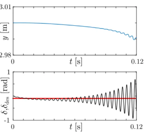
Fig. 9. Time profiles for the centre of gravity’s lateral position (upper panel) and the desired (thick red) and actual (thin black) steering angles (lower panel) for control parameterskψ= 0.5,ky = 0.05 1/m,p= 4000 and time-delaysτ1= 0.2 s,τ2= 0.001 s.

linear piecewise-smooth tire characteristics might reveal

‘bistable’ parameter domains where a stable equilibrium and a stable periodic solution coexist. This behavior con- sidered to be dangerous from engineering point of view as the domain of attraction of the stable equilibrium can be limited. On the other hand, one may need to consider possible saturations of the actuators which can also lead to complex dynamical phenomena.

ACKNOWLEDGEMENTS

This research has been supported by the New National Ex- cellence Programme of the Hungarian Ministry of Human Resources ´UNKP-17-3-I.

REFERENCES

De Sapio, V. (2017). Advanced Analytical Dynamics:

Theory and Applications. Cambridge University Press.

Falcone, P., Borrelli, F., Asgari, J., Tseng, H.E., and Hrovat, D. (2007). Predictive active steering control for autonomous vehicle systems. IEEE Transactions on Control Systems Technology, 15(3), 566–580.

Gantmacher, F. (1975).Lectures in Analytical Mechanics.

MIR Publishers.

Insperger, T. and St´ep´an, G. (2013). Semi-Discretisation for Time-Delay Systems. Springer.

Jalali, M., Khajepour, A., Chen, S., and Litkouhi, B.

(2017). Handling delays in yaw rate control of electric vehicles using model predictive control with experimen- tal verification. Journal of Dynamic Systems, Measure- ment, and Control, 139(12), 121001.

Kayacan, E., Ramon, H., and Saeys, W. (2016). Robust trajectory tracking error model-based predictive control for unmanned ground vehicles. IEEE/ASME Transac- tions on Mechatronics, 21(2), 806–814.

Pacejka, H. (2012). Tire and Vehicle Dynamics. Elsevier.

Shuai, Z., Zhang, H., Wang, J., Li, J., and Ouyang, M.

(2014). Combined AFS and DYC control of four-wheel- independent-drive electric vehicles over CAN network with time-varying delays. IEEE Transactions on Vehic- ular Technology, 63(2), 591–602.

St´ep´an, G. (1989). Retarded Dynamical Systems: Stability and Characteristic Functions. Longman.

Trefethen, L.N. (2000).Spectral Methods in Matlab. SIAM.

Ulsoy, A.G., Peng, H., and C¸ akmakci, M. (2012). Auto- motive Control Systems. Cambridge University Press.

Appendix A. COEFFICIENTS IN THE TIRE-FORCE CHARACTERISTICS

The coefficients in the tire force and self aligning torque characteristics in (6) and (7) can be expressed as

φ1= 2a²k, (A.1)

φ2=−8a⁴k²

3Fzµ0 +4a⁴k²µ

3Fzµ²₀, (A.2) φ3=−8a⁶k³

9F_z²µ²₀ −16a⁶k³µ

27F_z²µ³₀ (A.3) and

µ1=−2

3a³k, (A.4)

µ2= +8a⁵k² 3Fzµ0

−4a⁵k²µ

3Fzµ²₀ , (A.5) µ3=−8a⁷k³

9F_z²µ²₀ +16a⁷k³µ

9F_z²µ³₀ , (A.6) µ4= +64a⁹k⁴

81Fz³µ³₀ −16a⁹k⁴µ

9Fz³µ⁴₀ , (A.7) where a is the contact patch half-length, k is the dis- tributed lateral stiffness of the tires,Fz is the vertical load on the axles,µandµ0are the friction coefficients between the tires and the road for sliding and rolling, respectively.

Appendix B. COEFFICIENT MATRICES OF THE LINEARIZED SYSTEM

The coefficient matrices in (21) can be expressed as

A0=





















a11 a12 a13 0 0 0 a17 −kiϑ a21 a22 a23 0 0 0 a27 −kiθ a31 a32 a33 0 0 0 a37 kiΘ

0 0 0 0 0 0 0 0

1 0 0 0 0 V 0 0

0 1 0 0 0 0 0 0

0 0 1 0 0 0 0 0

0 0 0 0 0 0 0 0





















, (B.1)

where

Θ = JF(m+mF) + ∆

JF∆ , θ=m+mF

∆ , ϑ=−(l−d)mF

∆ (B.2) while

a11=−2a²k(6JG+ (a+ 3l)(l−d)mF)

3V∆ , (B.3)

a12=−V

+2ka² −3JG(2a−2d+l) + (a−d)(d−l)(a+ 3l)mF

3V∆ ,

(B.4) a13=−2a³kJG

V∆ , (B.5)

a17=2a²kJG

∆ , (B.6)

a21= 2a²k (6d−3l+a)m+ (3l+a)mF

3V∆ , (B.7)

a22= 2a²k (a²+ 5da−6d²−3al+ 6dl−3l²)m + (a−d)(a+ 3l)mF

/(3V∆), (B.8)

a23=2a³k(d−l)m

V∆ , (B.9)

a27=2a²k(l−d)m

∆ , (B.10)

a31= 2a²k −(a+ 3l)mF+ (3l−6d−a)m

JF+a∆

3V∆JF

, (B.11) a32= 2a²k

(−a²−5da+ 3al+ 6d²+ 3l²−6dl)m + (d−a)(3l+a)mF

JF+a(a−d+l)∆

/ (3V∆JF),

(B.12) a33=2a³k 3a(l−d)mJF+a∆

3V∆JF

, (B.13)

a37=2a³k 3a(l−d)mJF+a∆

3∆JF

, (B.14)

and

∆ = (d−l)²mFm+ (mF+m)JG. (B.15) Moreover, we have

A2=





















0 0 kdϑ 0 0 0 kpϑ 0 0 0 kdθ 0 0 0 kpθ 0 0 0 −kdΘ 0 0 0 −kpΘ 0

0 0 0 0 0 0 0 0

0 0 0 0 0 0 0 0

0 0 0 0 0 0 0 0

0 0 0 0 0 0 0 0

0 0 0 0 0 0 −1 0





















, (B.16)

A12=





















kdkyϑ kdkψϑ 0 0 kpkyϑ kd(kψ+kyV)ϑ 0 0 kdkyθ kdkψθ 0 0 kpkyθ kd(kψ+kyV)θ 0 0

−kdkyΘ −kdkψΘ 0 0 −kpkyΘ −kd(kψ+kyV)Θ 0 0

0 0 0 0 0 0 0 0

0 0 0 0 0 0 0 0

0 0 0 0 0 0 0 0

0 0 0 0 0 0 0 0

0 0 0 0 −ky −kψ 0 0



















 .

(B.17)