Multicriteria decision making for evergreen problems in food science by sum of ranking differences

(1)

Food Chemistry 344 (2021) 128617

Available online 12 November 2020

Multicriteria decision making for evergreen problems in food science by sum of ranking differences

Attila Gere

^a

, Anita R ´ acz

^b

, D ´ avid Bajusz

^c

, K ´ aroly H ´ eberger

^b^,^*

aSensory Laboratory, Institute of Food Technology, Szent Istv´an University, Vill´anyi út 29-43., 1118 Budapest, Hungary

bPlasma Chemistry Research Group, Research Centre for Natural Sciences, H-1117 Budapest, Magyar tud´osok krt. 2, Hungary

cMedicinal Chemistry Research Group, Research Centre for Natural Sciences, H-1117 Budapest, Magyar tud´osok krt. 2, Hungary

A R T I C L E I N F O Keywords:

Pareto optimization Food quality

Multiobjective decision making Food engineering

Food microbiology Quality control Sensory evaluation

A B S T R A C T

Finding optimal solutions usually requires multicriteria optimization. The sum of ranking differences (SRD) algorithm can efficiently solve such problems. Its principles and earlier applications will be discussed here, along with meta-analyses of papers published in various subfields of food science, such as analytics in food chemistry, food engineering, food technology, food microbiology, quality control, and sensory analysis. Carefully selected real case studies give an overview of the wide range of applications for multicriteria optimizations, using a free, easy-to-use and validated method. Results are presented and discussed in a way that helps scientists and practitioners, who are less familiar with multicriteria optimization, to integrate the method into their research projects. The utility of SRD, optionally coupled with other statistical methods such as ANOVA, is demonstrated on altogether twelve case studies, covering diverse method comparison and data evaluation scenarios from various subfields of food science.

1. Introduction

A well-formulated definition of food science tells us that “Food sci- ence is the study of the biological, chemical and physical properties of foods and their effects on the culinary, nutritional, sensory, storage and safety aspects of foods and beverages.” (Marcus, 2014). It is easy to accept even from this definition, or from personal experience, that food scientists use a diverse set of instruments to measure various food properties. The high number of different measurements comes from several subfields of food science, such as food engineering, food microbiology, or sensory analysis, just to name a few. Although the measurements originate from different sources, they all need to be analyzed with some kind of a data analysis method. The specific characteristics of the datasets from the different fields can be analyzed by chemometric, sensometric, biometric approaches, etc. However, one specific problem that emerges in all food science subfields is optimization. Optimization is one of the most common processes within the sub-disciplines of food science. Food scientists regularly face the question of how to choose the best process/model/pa- rameters, etc. from the many available alternatives.

This problem is well-known and is frequently called multiobjective or multi-parameter optimization (MOO or MPO), post-Pareto optimization (PPO) or preferably, multicriteria decision making (MCDM). In

multiobjective optimization, when the different objectives are contradictory, an optimal solution is said to be Pareto-optimal, when it is not possible to improve one objective without degrading the others (Benson, 2009).

In other words, we aim to choose the best of many alternatives by considering multiple input variables (Hendriks, de Boer, Smilde, &

Doornbos, 1992). In these situations, MCDM methods based on mathe- matically sound approaches (Bystrzanowska & Tobiszewski, 2018) can be applied, especially if

i. the decision process is complicated;

ii. there are many (virtually infinite) possible decision options;

iii. the decision process is “multistage”, or stepwise;

iv. the decision problem is highly important;

v. the decision relates to high profits or losses;

vi. subjectivity is difficult to be excluded (i.e. virtually always).

The application of MCDM methods increases the reliability of the decision (e.g. supports the notion that the chosen alternative is the best one) by giving clear and straightforward decision rules. However, most MCDM tools also necessarily introduce some level of subjectivity with the usage of arbitrary weights, even though it is preferable to avoid

* Corresponding author.

E-mail address: heberger.karoly@ttk.hu (K. H´eberger).

Contents lists available at ScienceDirect

Food Chemistry

journal homepage: www.elsevier.com/locate/foodchem

https://doi.org/10.1016/j.foodchem.2020.128617

Received 16 July 2020; Received in revised form 8 October 2020; Accepted 8 November 2020

(2)

weighting in the optimization process. On the other hand, these tools help in situations, when the objectives are conflicting and the results are diverse.

The high number of MCDM methods, while commendable, unavoidably results in a “confusion of abundance”. The question of how to select the “best” multi-criteria decision-making method has engaged the imagination of researchers for a long time (Ozernoy, 1992). In a recent paper, a set of 56 available MCDM methods was analyzed and a general framework, a formal guideline for MCDM method selection was proposed, which can be applied independently of the problem formulation (Wątrobski, Jankowski, Ziemba, Karczmarczyk, ´ & Zioło, 2019).

Nonetheless, these guidelines are somewhat hard to follow, because of a lack of proper software and the specificity of the MCDM problems.

Instead, a fully general MCDM tool would be desirable which is easily understandable, and can achieve a Pareto-optimal solution.

Some of the frequently applied multicriteria decision making algorithms are listed below: Desirability function analysis (desirability approach)–Aggregation of individual desirability functions: 0 <D <1 (Derringer & Suich, 1980); DRAPE (Deep ranking analysis by power eigenvectors) (Todeschini, Grisoni, & Ballabio, 2019); ELECTRE (Elim- ination and choice expressing the reality) (Roy, 1968); FDM (Fuzzy Decision Making) (Bellman & Zadeh, 1970); Kim and Lin criterion (KL)–

maximizes the minimum degree of satisfaction (Kim & Lin, 2000);

MAUT (Multi-attribute utility theory) (Sarin, 2013); MOORA (Multi- objective optimization on the basis of ratio analysis) (Brauers Willem, 2006); PROMETHEE II. (Preference ranking organization method for enrichment evaluations, modified version) (Brans & De Smet, 2016);

QLF (The quality loss function) (Kiran, 2017); TOPSIS (Technique for order of preference by similarity to ideal solution) (Hwang, Lai, & Liu, 1993). However, they apply various weighting schemes and produce different results, therefore it is difficult to find an optimal one among them.

Clear and unambiguous evidences have shown that sum of ranking differences (SRD) realizes a multicriteria optimization (Lourenço &

Lebensztajn, 2018; R´acz, Bajusz, & H´eberger, 2015; Sipos, Gere, Popp, &

Kov´acs, 2018; Stamenkovic et al., 2020). Lourenço and Lebensztajn have demonstrated on two practical examples that SRD realizes a consensus of eight MCDM methods, whereas any individual one “cuts out” a different part of the Pareto front as optimal. This limits the individual usage of MCDM tools, along with the subjectivity of weighting.

In this paper, we collected real-world situations in food science, to demonstrate how we can avoid the “confusion of abundance” of MCDM choices, using a simple and easy-to-use technique, sum of ranking differences (SRD).

2. Methods

2.1. Sum of ranking differences (SRD)

Over the past ten years, sum of ranking differences (SRD) has become a widely used approach to solve multicriteria optimization problems in many disciplines. It was introduced in 2010 (H´eberger, 2010) along with practical examples, and its validation protocol was established based on a randomization test. Briefly, SRD relies on comparing the ranking of objects by the various methods/alternatives to a reference ranking, ac- quired from either a “golden standard” method or a consensus (i.e.

average, minimum, maximum, etc.) of the individual rankings. The resulting “sum of ranking differences” values measure the closeness of the individual rankings to the reference, therefore SRD can solve method-comparison problems in a fast and easy way: the smaller the sum, the better the method (i.e. the closer it is to the golden standard or consensus). Originally, validation was performed by running SRD on randomly generated datasets of the same size as the input data matrix.

The obtained histogram shows whether the ranking is comparable with random ranking (e.g. when the original variables overlap with the random distribution). In addition, theoretical SRD distributions were

determined for different sample sizes up to 13. The resulting randomization test was termed “comparison of ranks with random numbers”

(CRRN) and was introduced in 2011. It was shown that the theoretical SRD distribution is asymmetric and discrete for small sample sizes, but it can be approximated well with a normal distribution for sample sizes larger than 13 (Héberger & Kollár-Hunek, 2011). An important step was the extension of SRD to handle repeated observations (ties) in the dataset. Ties occur when multiple objects have the same raw value and therefore cannot be ranked; in such situations, partial rankings should be used. It is especially problematic if ties are present in the reference (golden standard) vector. A new algorithm was developed to define the theoretical SRD distributions with ties. Here, exact theoretical distributions were determined for 4 <n <9 and a reasonable approximation is provided for n >8 using Gaussian distributions fitted on three million n–dimensional random vectors (Kollár-Hunek & Héberger, 2013). The latest results have cleared up how to choose the proper cross-validation variant for SRD, e.g. k-fold contiguous or repeated resampling (with return), number of folds (5 <k <10), etc. Briefly, the methods/models are analyzed with factorial analysis of variance (ANOVA), with the following factors: i) contiguous or resampling, ii) k-folds: 5–10, iii) number of methods/models, i.e. columns in the input matrix (Héberger

& Koll´ar-Hunek, 2019). All details, along with a manual can be found in

the literature sources mentioned in this section. An MS Excel Visual Basic macro, together with example input and result files are down- loadable from: http://aki.ttk.mta.hu/srd. Additionally, we have extended the availability of SRD to other popular platforms such as R Shiny (https://attilagere.shinyapps.io/srdonline/) and Jupyter Note- book (https://github.com/davidbajusz/srdpy).

2.2. Analysis of variance (ANOVA)

Somewhat contrary to what its name suggests, ANOVA is a group of statistical methods based on the pairwise comparison of the average values of different groups of samples. In its most basic realization, ANOVA generalizes the two-sample t-test to more groups, by establish- ing the statistical significance of different group averages at a given error level. Therefore, it is an ideal method to combine with sum of ranking differences (SRD), to establish whether the SRD values for the compared methods are significantly different (pair- or groupwise), or not. Contrary to traditional ANOVA, a positive quality can be attributed to the magnitude of the SRD scores, with the smaller being the better (i.e.

closer to the reference, benchmark). To obtain the uncertainties of SRD values for each compared method, n-fold (usually sevenfold) cross- validation is performed on the original input matrix (or leave-one-out cross-validation, if the number of rows is small), resulting in n SRD values per method (or k in case of leave-one-out, where k is the total number of rows). The resulting averages are then compared pair- or groupwise in the framework of ANOVA, either with simple t-tests, or more advanced post-hoc analogs, such as Tukey’s HSD test, which is applied in the case studies presented here (Tukey, 1949). ANOVA is implemented in most of the current statistical software suites, as well as freely available modules of major data science platforms such as Python;

here, we have used STATISTICA 13 (TIBCO Software Inc., www.tibco.

com, USA). Additionally, ANOVA can be applied in more advanced setups (factorial ANOVA) to dissect the overlapping effects of more, independent factors on the group averages; we refer to our recent cheminformatics study as an example (R´acz, Bajusz, & H´eberger, 2018).

2.3. Selection of case studies

In order to showcase the wide applicability of the SRD technique, a range of case studies were collected and re-analyzed using SRD. As food science covers a wide range of subdisciplines, the following areas have been selected: analytics in food chemistry, food engineering, food technology, food microbiology, food quality control and food sensory analysis. The chosen papers should: i) fit clearly into one of the defined

(3)

subfields; ii) contain research data with sufficient number of samples (suitable table for SRD analysis).

3. Case studies

3.1. Analytics in food chemistry

A broad field of food chemistry deals with the determination of micro- and/or macro-nutrients, which provides essential information for nutritionists and food product developers on specific products, varieties, etc. However, comparison of multiple samples based on multiple attri- butes (e.g. micro- or macronutrients) is somewhat challenging, since there are no clear winners in most cases. Here, we provide a solution to such problems with sum of ranking differences (SRD), illustrated with two case studies.

3.1.1. Plant protein amino acid profiles

Eight plant proteins were compared based on their amino acid profiles published by (S´a, Moreno, & Carciofi, 2020). The authors presented the nutritional and amino acid compositions of the following legumes:

soybean (Glycine max L.), bean (Phaseolus vulgaris), pea (Pisum sativum), faba bean (Vicia faba), chickpea #1 (Cicer arietinum), chickpea #2 (Cicer arietinum), cowpea (Vigna unguiculata) and lupin (Lupinus angustifolius).

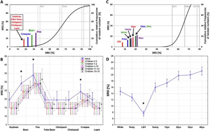
The amino acid profiles have been compared to the recommended amino acid intake scoring patterns from the WHO/FAO/UNU Expert Consul- tations (2007) for all age groups (0.5 years, 1–2 years, 3–10 years, 11–14 years, 15–18 years and over 18 years). SRD results are summa- rized in Fig. 1. Fig. 1A presents the scaled SRD values, with the recommended amino acid intake pattern for adults as the reference vector.

Legumes that are closer to the origin are more similar to the reference

amino acid pattern. The ranking clearly shows that soybean, faba bean, chickpeas and lupin have the most similar amino acid profiles to the reference, while cowpea, bean and pea show decreasing similarities, respectively. Based on the presented results, adults should preferably choose legumes from the first four plant proteins when their amino acid profile is of importance. Fig. 1B presents the analysis of variance (ANOVA) results of the 7-fold cross-validated SRD values for all WHO age groups. The plot shows similar patterns as observed for adults: the same four legumes are the most recommended for children of all age groups. The generally larger SRD values point out that there are larger differences of the legume amino acid profiles from the adult reference intake data, suggesting that the legumes, on average, are more compatible with the recommended amino acid intake values of children.

Comparing Fig. 1A and B to the bar plots presented in Fig. 1 of (S´a et al., 2020), we can conclude that SRD enhances not only the quality of data analysis, but the visualization possibilities as well. It is important to highlight that these recommendations are based on the results of eight legumes, considering solely their amino acid profiles. (Including further micro- and/or macronutrients in the analysis might give different results.)

3.1.2. Volatile organic compound analysis of wines

Another important subfield of food chemistry covers the volatile organic compound (VOC) analysis of food products. VOCs play an important role in consumer acceptance (Aisala et al., 2020), and also in food quality and safety (Radv´anyi, Gere, Jokai, ´ & Fodor, 2015). Moreira et al. (2019) used headspace solid phase microextraction sampling with gas chromatography and mass spectrometry (HS-SPME-GC–MS) to quantify volatile carbonyl compounds in Port wines (Moreira et al., 2019). They present the concentrations of volatile compounds in eight

Fig. 1. Scaled (0–100) sum of ranking differences (SRD) values for the plant protein (A) and port wine (C) datasets. The reference column was defined as the WHO amino acid reference intake values for adults for the former (A), and the row minimums for the latter (C). Scaled SRD values are plotted on x and left y axes, while the right y axis shows the cumulative relative frequencies for random rankings (black curve, the 5% (XX1), Median (Med), and 95% (XX19) values are also indicated).

Analysis of variance of cross-validated SRD values for the plant protein (B) and port wine (D) datasets. “*” indicates significantly different samples (no overlapping groups) determined by Tukey’s HSD post hoc test, here and in all further figures.

(4)

Port wine categories: white, Tawny (Tawny, 10, 20, 30 and 40 years old) and Ruby (Ruby and Late Bottled Vintage (LBV)). During the analysis of the dataset, which contains the concentrations of 37 compounds, we aimed to find rank patterns of the samples based on their total VOC content, from minimum to maximum. Reference values were set to row minimums; hence, the sample closest to the zero SRD value contains the lowest amount of VOCs. It is expected to find young wines closer to zero, while barrel-aged, older samples are expected to have higher SRD values. Fig. 1C shows that late bottled vintage (LBV) is the closest to the zero point and the amounts of VOCs gradually increase with aging, as expected. In order to identify characteristic groups in the dataset, ANOVA coupled with LSD post hoc tests was applied to the sevenfold cross-validated SRD results. Fig. 1D indicates that three groups are present in the data set: LBV; white and ruby; and Tawny samples.

However, a clear difference (homogenous subgroups without overlap) was observed only in the case of LBV, the sample containing the lowest total amount of VOC. In this case study, SRD was able to rank and group the wines based on their VOC content. Such applications of SRD give the researchers instant feedback on the characteristic groups of samples that are present in the dataset.

3.2. Food engineering

We selected two common comparison problems from food engineering. On one hand, comparison of different models based on their prediction or classification performances are key in food engineering projects to define the best processes or to choose the best prediction method. On the other hand, SRD can also be applied to decompose the effects of sub-steps on an overall process, as illustrated with the food waste treatment dataset in Section 3.2.2 (ranking the sub-steps of

anaerobic digestion in terms of environmental impact).

3.2.1. Biochemical reaction dataset

In a 2007 study, Bas and Boyaci investigated the effects of pH and substrate concentration on the reaction rate of the amyloglucosidase enzyme by conducting experiments according to a face-centered design (FCD) and a modified face-centered design (MFCD). The data was then used to predict amyloglucosidase enzyme concentrations using response surface methodology (RSM) and artificial neural network (ANN) (Bas &

Boyaci, 2007). The authors compared the results of the four configurations (two designs, and two models) to the measured response, which is a suitable input data matrix for SRD. Fig. 2A shows that ANN with the MFCD design obtained the lowest SRD value, followed by RSM_FCD, ANN_FCD and RSM_MFCD, respectively. Although the figure suggests a grouping of the methods, ANOVA of the leave-one-out cross-validated SRD values proves that ANN_MFCD gave significantly more accurate predictions than the other three configurations (Fig. 2B). Additionally, the other three show no significant differences, meaning that their performances are close to identical. Our results are in accordance with the conclusions of the authors, additionally presenting the comparison of the two designs.

3.2.2. Food waste treatment dataset

A study comparing five food waste treatment methods was published by Gao et al. in 2017. The authors compared anaerobic digestion, landfill, incineration, composting and heat-moisture reaction based on the amounts of emitted substances to air and water. Additionally, the six consecutive steps constituting the complete waste treatment cycle of anaerobic digestion (from food waste collection to post-processing by dehydration) were analyzed in the same manner. As SRD requires a

Fig. 2. Scaled (0–100) sum of ranking differences (SRD) values for the biochemical reaction dataset (A). Measured enzyme reaction responses were used as the reference (benchmark) column. SRD plots are explained in the caption of Fig. 1. ANOVA results for the biochemical reaction dataset (B) and the food waste treatment dataset (C: consecutive steps of anaerobic digesting, D: comparison with other alternatives).

(5)

reference column to compare the different treatment methods, the minimum was chosen, i.e. the (hypothetical) treatment emitting the smallest amount of substances into the air is selected to be the standard (Gao, Tian, Wang, Wennersten, & Sun, 2017). Fig. 2C presents the ANOVA results of the leave-one-out cross-validated SRD values of the consecutive steps of anaerobic digestion, which clearly shows that transporting the waste to the local waste treatment facility has overall the lowest impact on the amounts of emitted substances. Based on Tukey’s HSD post hoc test, three clusters can be perceived. Dehydrating received the second lowest SRD value (after transporting), followed by the group of other processes, showing no significant differences among themselves. When the complete processes of five different food waste treatment cycles are compared (Fig. 2D), anaerobic digestion has clearly proven to be the best with an SRD =0 value. The zero SRD value means that this treatment method has the same ranking of the evaluated substances as the reference (minimum). These findings are not only in accordance with those reported by the authors, but leave-one-out cross- validation of the SRD values gives a further option for graphical depic- tion, and can also establish statistical relations (significant or non- significant difference) between the compared methods (Fig. 2D).

3.3. Food technology

Optimization of technological parameters is often required in food technology. In many cases, there are multiple methods with several possible settings. Sum of ranking differences handles the comparison of these kinds of measurements well, by comparing the methods and their settings. (Obviously, this means that the number of columns in the input SRD table increases.)

3.3.1. Optimization of solid phase microextraction (SPME) sampling The author of this study used two SPME fibers and three sampling times to collect as much volatile compounds from foal dry-cured loin as possible (Lorenzo, 2014). The combination of fiber type and sampling time resulted in six columns in the SRD input table, while the amounts of extracted compounds by type (acids, alcohols etc.) served as the basis of the comparison (Table 2 of Lorenzo (2014)). Maximum was chosen as the reference, since we are looking for the fiber type and sampling time combination, which absorbs the most compounds in a short time period.

SRD analysis revealed that Carboxen/Polydimethylsiloxane (CARPDMS) fiber with a 45-minute sampling time (CARPDMS45) received the lowest SRD value, i.e. this sampling method was closest to the reference column. Naturally, more compounds are absorbed over a longer sampling time, however, our result also proved that CARPDMS fibers gave lower or equal SRD values compared to fibers from Divinylbenzene/Carboxen/

Polydimethylsiloxane (DVDCARPDMS) (Fig. 3A). The ANOVA plot of the cross-validated SRD results supported these: CARPDMS45 showed not only the lowest SRD values but the lowest standard deviation as well (Fig. 3B). The presented results demonstrate that SRD gives valuable help in SPME sampling optimization by providing a clear rank of the analyzed combinations and a statistical analysis of the ranks.

3.3.2. Drying kinetics dataset

When it comes to technological method optimization, it is also possible to combine and compare more settings simultaneously, as exemplified by the authors of a recent study, where different settings of convective drying of raspberries were compared to freeze drying (Sta- menkovic et al., 2020). Fresh and frozen raspberries were dried at three different temperatures, at two air rates, yielding a total of 12 combinations of drying conditions, which were compared to the industry reference freeze drying. SRD analysis resulted in a clear winner, freshly

Fig. 3. Scaled sum of ranking differences (SRD) values for the solid phase microextraction optimization dataset (A) and the drying kinetics dataset (C). For the reference column, row maximums (A) and freeze-drying results (C) were used, respectively. SRD plots are explained at Fig. 1. ANOVA results for the solid phase microextraction optimization dataset (B) and the drying kinetics dataset (D). Abbreviations: CARPDMS, Carboxen/Polydimethylsiloxane; DVDCARPDMS, Divinyl- benzene/Carboxen/Polydimethylsiloxane; numbers after SPME fiber names denote sampling time in minutes, panels (A, B). Raspberry sample names are coded by stage (Fro: frozen, Fre: fresh), air temperature in Celsius (60, 70 and 80), and applied air rate in m s⁻¹(0.5 and 1.5), panels (C, D).

(6)

dried raspberries at 60 ^◦C and 1.5 m⋅s⁻¹air rate, meaning that based on the physical, chemical and technological measurements (such as moisture content, volume, total phenolic content, etc.), this drying method is the most similar to freeze drying (Fig. 3C). ANOVA analysis reveals a pattern in the cross-validated SRD values, since all combinations with a drying temperature of 60 ^◦C received significantly lower SRD values than the other temperatures (Fig. 3D). Additionally, fresh samples resulted in SRD values lower than or equal to that of frozen samples, indicating that sample pre-treatment has a significant effect on the drying kinetics.

Such optimization studies are commonly done in food sciences. Here, the application of SRD would increase the reliability of the conclusions and would support the decisions by statistical tests. Therefore, SRD is not only a suggested research tool, but a great method for practitioners, who want to validate new methods, treatments, or techniques, and compare them to existing industrial references.

3.4. Food microbiology 3.4.1. Bacillus isolates dataset

In food microbiology, the number of colony-forming units (cfus) on a media is indicative of the effectiveness of a given food preservation technique. The following example considers the data presented by Ronimus et al. (2003). The authors investigated antibiotic sensitivities of seven major groups of dairy-derived Bacillus isolates. The presented data table gives the diameters of inhibitory zones in millimeters. SRD was employed to discover which isolate shows the lowest sensitivity, i.e.

which isolate is the least sensitive to the antibiotics. Fig. 4A presents the SRD results, where the minimum was used as the reference, hence isolates closer to zero SRD provided the smallest diameters of inhibitory zones. The two isolates of Bacillus licheniformis showed clearly the lowest

SRD values, thereby being the most resistant to the examined antibiotics.

As these isolates are placed before the XX1 line (5% significance), the provided ranks are significant. All the other isolates are placed right from XX1, meaning that their ranking is not significantly different from random ranking. Fig. 4B supports the above-mentioned results, however, after leave-one-out cross-validation, Bacillus subtilis forms an intermittent third group, with SRD values higher than that of B. licheniformis isolates, but significantly lower than that of the other isolates.

3.4.2. Fermented sausages dataset

In a recent study, five curing formulations of fermented sausages prepared from fallow deer and beef were compared, by varying the amount and composition of the applied salt (curing salt vs. sea salt), and acid whey powder (amounts equivalent to 0, 5, 10 or 20% liquid acid whey) (Kononiuk & Karwowska, 2020). In order to avoid missing data rows, measurement data from day 0 were collected from the paper for the following variables: oxidation–reduction potential (ORP), lactic acid bacteria and Enterobacteriaceae content, tyramine, spermidine and spermine content. Data of beef and fallow deer samples were both used in order to give a cross-sample comparison of the treatments. Due to the different scales of measurements, normalization was applied. For reference, the row minimum was chosen since the expected values of all these variables should be as low as possible to ensure food safety. Results presented by Fig. 4C indicate that SAW2 (tested sample with 2.8% sea salt and an amount of acid whey powder corresponding to 10% liquid acid whey) provided the lowest SRD result, meaning that overall it had the lowest values of the input variables. Fig. 4D highlights that after leave-one-out cross-validation, SAW2 cannot be differentiated from the control sample (prepared with curing salt); on the other hand, all the other samples show significantly higher SRD values.

Fig. 4. Scaled sum of ranking differences (SRD) values for the antibiotic sensitivities dataset (A) and the uncured fermented sausages dataset (C). For the reference column, row minimums were used in both cases. SRD plots are explained at Fig. 1. ANOVA results for the antibiotic sensitivities dataset (B) and the uncured fermented sausages dataset (D). Abbreviations: sample codes (A-G); B.st, B. stearothermophilus; A.fl, A. flavothermus; B.l, B. licheniformis in panels (A,B). C (control sample with 2.8% curing salt); S (reference sample with 2.8% sea salt); SAW, SAW2 and SAW4 (tested sample with 2.8% sea salt and 5%, 10% and 20% liquid acid whey- equiv. whey powder), in panels (C, D).

(7)

3.5. Food quality control

In food quality control, there are several situations when large amounts of data are generated, highlighting the importance of multivariate data analysis to extract relevant information. Two case studies of such scenarios follow.

3.5.1. Near infrared spectroscopic analysis of Q10 capsules

One of the most obvious cases is near infrared spectroscopy (NIRS), which almost always requires multivariate statistics/modelling. In this case study (R´acz, Vass, H´eberger, & Fodor, 2015), the authors analyzed 50 different capsules/tablets of dietary supplements to model their coenzyme Q10 concentrations. Since NIRS is not able to directly measure the concentration of exact compounds, additional measurements are required, which are usually slower and more expensive. In this specific case, high performance liquid chromatography (HPLC) measurements were conducted to determine the reference values (or, with regression terms, the dependent variable), i.e. the amount of Q10 in the capsules (coded as Exp in Fig. 5). Partial least squares regression was used to build a prediction model based on the NIR spectra as independent variables and the measured Q10 concentrations as the dependent variable.

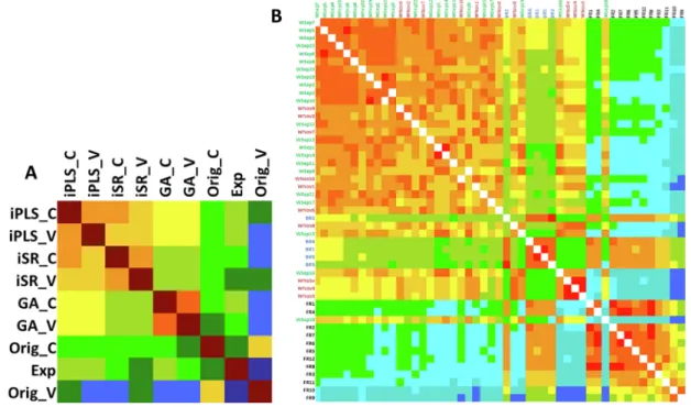
The authors evaluated the performances of different variable selection methods, such as interval partial least squares regression (iPLS), interval selectivity ratio (iSR) and genetic algorithms (GA), compared to using the original data set without variable selection (Orig). The selected variables were used for PLS regression and the predicted Q10 concentrations were subjected to SRD analysis. (Both the calibration and validation results were included, denoted by “C” and “V”, respectively.) Fig. 5A presents the heatmap representation of the SRD results, where each of the available methods, in turn, are used as the reference method.

Warmer colors mean lower SRD values, indicating that the tested variable selection method (row) showed similar results to the reference (column). The heatmap is arranged according to the averages of the row/columns, i.e. methods on the top/left are more consistent on average with the rest of the available methods, while outliers are located on the bottom/right. iPLS provided the lowest SRD values overall, both

the calibration and validation sets are ranked ahead of the other methods. Naturally, calibration sets give more accurate results, while validation sets usually show a slight drop in their performance. We can conclude that variable selection is always favorable, since all variable selection methods are ranked ahead of the original data set (without variable selection) on Fig. 5A.

3.5.2. Authentication of game meat

The second publication deals with the authentication of game meat through rare earth element fingerprinting (Danezis et al., 2017), with 39 elements measured in three types of rabbit meat (wild, backyard-raised and farmed), harvested on different days. Fig. 5B presents the heatmap of SRD values, assigning warmer colors to the samples with an element pattern closer to the rest of the samples on average. Wild rabbit samples are placed in the upper left corner of the plot, followed by backyard- raised rabbit samples and farmed samples show the least similarity to the rest on average. These results indicate that backyard-raised rabbits show a higher similarity to the wild ones in terms of their rare earth element content.

3.6. Food sensory analysis

A great advantage of the SRD method is that the transpose of the input data table might be useful as well. This way, SRD provides even more information, by comparing not only the methods, but also the samples of the input data table.

3.6.1. Evaluation of just-about-right scales

An interesting example is presented from the field of sensory analysis, where the performance of just-about-right (JAR) evaluation methods was tested (Gere, Sipos, Kovács, Kókai, & Héberger, 2017). The authors used eight methods to assess the effect of twelve sensory attributes on overall liking. First, the JAR variables were placed in the columns and the evaluation methods in the rows as the input for the SRD calculation (Fig. 6A). Here, the maximum was used as the reference, since we were looking to find the most influential variables. Our results

Fig. 5.Heatmap of the scaled SRD values of the Q10 capsules data set (A) and the game meat authentication data set (B). Smaller SRD values receive warmer color, the heatmap is arranged from smaller to larger average SRD values (top to bottom, left to right). Abbreviations: iPLS, interval partial least squares regression; iSR, interval selectivity ratio; GA, genetic algorithm; Orig, data set without variable selection; Exp, Q10 concentration measured by HPLC method; C, calibration; V, validation in panel (A). W, wild rabbit; BR, backyard-raised rabbit; FR, farmed rabbit; harvest date (month, day) in panel (B).

(8)

show that not enough flavor intensity (denoted by a “–“ sign after the name of the attribute) was found to be the most influential sensory attribute, i.e. the lack of flavor intensity decreased the overall liking the most. The ranks of the attributes provide a clear order of importance for sensory specialists and food product developers about how to reformu- late their products to achieve higher consumer acceptance. Further- more, the results are based on the consensus of no less than eight methods. In the transposed input matrix, the JAR evaluation methods are enumerated in the columns and product attributes are placed in the rows; therefore, the consensus of the methods (reference column) is defined as the row average (Fig. 6B). A clear ordering of the methods can be established based on their SRD values (i.e. their city-block distances from the average result). As none of the methods are considered to be inferior or superior (most of them are part of the relevant ASTM standard as standard methods (Rothman & Parker, 2009)), we should consider their results to be good/valid. However, due to the methodo- logical differences, the results might even be contradictory sometimes.

SRD gives an outstanding possibility to determine, which method gives a result closest to the average. Here, generalized pair-correlation (GPCM) is recommended as the method closest to the average (Gere, Sipos, &

H´eberger, 2015).

3.6.2. Evaluation of Thurstonian d-prime values

As SRD was primarily developed for model comparison, it is a suitable tool to assess the performance of model parameters. As an example from the field of sensory analysis, we compared the variances of

Thurstonian d-prime values (Kuesten, Bi, & Meiselman, 2017) using SRD. The input SRD table lists eight mood states from the Profile of Mood States (POMS), along with their variances, in seven subgroups. We are looking for the most stable of those mood states, i.e. those that show the least variance among the subgroups. Fig. 6C presents the analysis of variance of the cross-validated (scaled) SRD values, where the lowest values correspond to the lowest variances. Interestingly, total mood disturbance (a calculated feature) showed the lowest Thurstonian d- prime variance, followed by figure-inertia. On the other side of the scale is vigor-activity, meaning that this mood state shows the highest variance among the different subgroups.

4. Conclusions

Carefully selected case studies of multicriteria decision making (MCDM) problems in food science were collected. Sum of ranking differences (SRD) has been introduced as an easy-to-use, freely available and scientifically sound alternative, proven to be a consensus of many MDCM techniques. The SRD algorithm has great potential in food science, by giving a clear ranking of the samples/methods in each case, and being easy to interpret and present. It is a nonparametric method, i.e.

there is no need to have normally distributed data. This is of high importance in food science, where normality generally cannot be assumed. The method can also be applied to extremely small datasets (n

>3), but the number of samples (rows) should be preferably seven or more, while the number of compared methods (columns) should be no Fig. 6. Scaled sum of ranking differences (SRD) values for the JAR attributes (A) and the evaluation methods (B) of the sensory method comparison dataset, with row maximums and minimums as the reference column, respectively. SRD plots are explained at Fig. 1. ANOVA results for the Consumers’ Profile of Mood States (POMS) dataset (C). The row minimums were used as reference (benchmark) column. In panel (A), the signs “+” and “− ” mean the too much and not enough endpoints of the just-about-right scales, respectively. Abbreviations: Ordinary least-squares regression, OLS; Penalty analysis, Penalty; Bootstrapping penalty analysis, bPenalty;

Generalized pair correlation method, GPCM; Partial least squares regression using dummy variables as dependent variable, PLS-dummy; Multiple linear regression, MLR; Penalty analysis for JAR mean method, wPAforJARMean; Weighted Penalty analysis for grand mean method, wPAforGrandMean in panel (B). Tension-Anxiety, TA; Depression-Dejection, DD; Anger-Hostility, AH; Vigor-Activity, VA; Figure-Inertia, FI; Confusion-Bewilderment, CB; Friendliness, FR; Total Mood Disturbance, TDM in panel (C).

(9)

less than three to obtain sensible results (although strictly speaking, it is possible to compare two methods, as well). As limited amounts of data can also be a problem in some areas of food science, this is also a great advantage.

Optimization problems are common in food science, where the application of the SRD method greatly increases the reliability of the results, and supports optimal decisions by correct statistical tests.

Therefore, SRD is not only a suggested research tool, but a great method for practitioners, who need to compare and validate new methods, treatments or techniques to existing industrial references. Most impor- tantly, it is an easy-to-use method for extracting meaningful conclusions from research data, that otherwise might not have been apparent to the practitioners. A small sample of our novel findings from the twelve case studies considered in this paper include: (i) legumes (esp. soybean, faba bean, chickpeas and lupin), are on average more compatible with the WHO-recommended amino acid intake values of children than adults, (ii) from food waste treatment methods, the results of SRD showed that anaerobic digestion is the most environmentally friendly, while there is no significant difference between composting and heat-moisture reaction in terms of emission profiles, (iii) among the major groups of dairy- derived Bacillus isolates, Bacillus licheniformis is the most resistant to antibiotics, followed by Bacillus subtilis, (iv) for producing fermented sausages, a formulation of 2.8% sea salt and 10% whey powder is the ideal choice for replacing the use of sodium nitrate without increasing the amount of biogenic amines.

SRD is available as a Microsoft Excel macro, which makes its application easy for non-statisticians and researchers less familiar with pro- gramming languages, and is freely available at http://aki.ttk.mta.hu/

srd. In addition, to make automation easier, Python- and R-project- based versions of SRD were introduced here and are being developed as well, freely available at https://github.com/davidbajusz/srdpy and htt ps://attilagere.shinyapps.io/srdonline/

CRediT authorship contribution statement

Attila Gere: Conceptualization, Methodology, Validation, Re- sources, Project administration. Anita Racz: Conceptualization, Meth-´ odology, Resources, Visualization. David Bajusz: ´ Software, Visualization. H´eberger Karoly: ´ Conceptualization, Methodology, Validation, Formal analysis, Funding acquisition.

Declaration of Competing Interest

The authors declare that they have no known competing financial interests or personal relationships that could have appeared to influence the work reported in this paper.

Acknowledgements

The authors thank the support of the National Research, Develop- ment and Innovation Office of Hungary (OTKA, contract No K119269 and K134260). The authors were supported by the European Union and co-financed by the European Social Fund (grant agreement no. EFOP- 3.6.3-VEKOP-16-2017-00005). AG thanks the support of Premium Postdoctoral Researcher Program of Hungarian Academy of Sciences.

DB is supported by the J´anos Bolyai Research Scholarship of the Hun- garian Academy of Sciences. AR is supported by the National Research, Development and Innovation Office of Hungary (PD 134416).

Data availability

Data is available as Supplementary material.

Appendix A. Supplementary data

Supplementary data to this article can be found online at https://doi.

org/10.1016/j.foodchem.2020.128617.

References

Aisala, H., Manninen, H., Laaksonen, T., Linderborg, K. M., Myoda, T., Hopia, A., &

Sandell, M. (2020). Linking volatile and non-volatile compounds to sensory profiles and consumer liking of wild edible Nordic mushrooms. Food Chemistry, 304, Article 125403. https://doi.org/10.1016/j.foodchem.2019.125403.

Bas, D., & Boyaci, I. H. (2007). Modeling and optimization II: Comparison of estimation capabilities of response surface methodology with artificial neural networks in a biochemical reaction. Journal of Food Engineering, 78(3), 846–854. https://doi.org/

10.1016/j.jfoodeng.2005.11.025.

Bellman, R., & Zadeh, L. (1970). Decision-making in a fuzzy environment. Retrieved July 6, 2020, from Management Science, 17(4), B141–B164 www.jstor.org/stabl e/2629367.

Benson, H. P. (2009). Multi-objective optimization: Pareto optimal solutions, properties pp. 2478-2481. In Christodoulos A. Floudas, & Panos M. Pardalos (Eds.), Encyclopedia of optimization. Boston (USA): Springer. https://doi.org/10.1007/978- 0-387-74759-0_426.

Brans, J.-P., & De Smet, Y. (2016). PROMETHEE methods. In S. Greco, M. Ehrgott, &

J. R. Figueira (Eds.), Multiple criteria decision analysis: State of the art surveys (pp.

187–219). https://doi.org/10.1007/978-1-4939-3094-4_6.

Brauers Willem, Z. E. (2006). The MOORA method and its application to privatization in a transition economy. Control and Cybernetics, 35(2), 445–469.

Bystrzanowska, M., & Tobiszewski, M. (2018). How can analysts use multicriteria decision analysis? TrAC - Trends in Analytical Chemistry, 105, 98–105. https://doi.

org/10.1016/j.trac.2018.05.003.

Danezis, G. P., Pappas, A. C., Zoidis, E., Papadomichelakis, G., Hadjigeorgiou, I., Zhang, P., … Georgiou, C. A. (2017). Game meat authentication through rare earth elements fingerprinting. Analytica Chimica Acta, 991, 46–57. https://doi.org/

10.1016/j.aca.2017.09.013.

Derringer, G., & Suich, R. (1980). Simultaneous optimization of several response variables. Journal of Quality Technology, 12(4), 214–219. https://doi.org/10.1080/

00224065.1980.11980968.

Gao, A., Tian, Z., Wang, Z., Wennersten, R., & Sun, Q. (2017). Comparison between the technologies for food waste treatment. Energy Procedia, 105, 3915–3921. https://doi.

org/10.1016/j.egypro.2017.03.811.

Gere, A., Sipos, L., & H´eberger, K. (2015). Generalized Pairwise Correlation and method comparison: Impact assessment for JAR attributes on overall liking. Food Quality and Preference, 43, 88–96. https://doi.org/10.1016/j.foodqual.2015.02.017.

Gere, A., Sipos, L., Kovács, S., Kókai, Z., & Héberger, K. (2017). Which just-about-right feature should be changed if evaluations deviate? A case study using sum of ranking differences. Chemometrics and Intelligent Laboratory Systems, 161, 130–135. https://

doi.org/10.1016/j.chemolab.2016.12.007.

H´eberger, K. (2010). Sum of ranking differences compares methods or models fairly.

TrAC - Trends in Analytical Chemistry, 29(1), 101–109. https://doi.org/10.1016/j.

trac.2009.09.009.

H´eberger, K., & Koll´ar-Hunek, K. (2011). Sum of ranking differences for method discrimination and its validation: Comparison of ranks with random numbers.

Journal of Chemometrics, 25(4), 151–158. https://doi.org/10.1002/cem.1320.

H´eberger, K., & Koll´ar-Hunek, K. (2019). Comparison of validation variants by sum of ranking differences and ANOVA. Journal of Chemometrics, 33(6). https://doi.org/

10.1002/cem.3104. e3104.

Hendriks, M. M. W. B., de Boer, J. H., Smilde, A. K., & Doornbos, D. A. (1992).

Multicriteria decision making. Chemometrics and Intelligent Laboratory Systems, 16(3), 175–191. https://doi.org/10.1016/0169-7439(92)80036-4.

Hwang, C.-L., Lai, Y.-J., & Liu, T.-Y. (1993). A new approach for multiple objective decision making. Computers & Operations Research, 20(8), 889–899. https://doi.org/

10.1016/0305-0548(93)90109-V.

Kim, K.-J., & Lin, D. K. J. (2000). Simultaneous optimization of mechanical properties of steel by maximizing exponential desirability functions. Journal of the Royal Statistical Society: Series C (Applied Statistics), 49(3), 311–325. https://doi.org/10.1111/1467- 9876.00194.

Kiran, D. R. (2017). Chapter 31 - Quality Loss Function. In D. R. Kiran (Ed.), Total Quality Management (pp. 439–445). https://doi.org/10.1016/B978-0-12-811035-5.00031-3.

Koll´ar-Hunek, K., & H´eberger, K. (2013). Method and model comparison by sum of ranking differences in cases of repeated observations (ties). Chemometrics and Intelligent Laboratory Systems, 127, 139–146. https://doi.org/10.1016/j.

chemolab.2013.06.007.

Kononiuk, A. D., & Karwowska, M. (2020). Comparison of selected parameters related to food safety of fallow deer and beef uncured fermented sausages with freeze-dried acid whey addition. Meat Science, 161. https://doi.org/10.1016/j.

meatsci.2019.108015.

Kuesten, C., Bi, J., & Meiselman, H. L. (2017). Analyzing consumers’ Profile of Mood States (POMS) data using the proportional odds model (POM) for clustered or repeated observations and R package ‘repolr’. Food Quality and Preference, 61, 38–49.

https://doi.org/10.1016/j.foodqual.2017.04.014.

Lorenzo, J. M. (2014). Influence of the type of fiber coating and extraction time on foal dry-cured loin volatile compounds extracted by solid-phase microextraction (SPME).

Meat Science, 96(1), 179–186. https://doi.org/10.1016/j.meatsci.2013.06.017.

Lourenço, J. M., & Lebensztajn, L. (2018). Post-pareto optimality analysis with sum of ranking differences. IEEE Transactions on Magnetics, 54(8), 1–10. https://doi.org/

10.1109/TMAG.2018.2836327.

(10)

Marcus, J. B. (2014). Nutrition basics: What is inside food, how it functions and healthy guidelines. In Culinary Nutrition (1st ed., pp. 1–50). https://doi.org/10.1016/b978-0- 12-391882-6.00001-7.

Moreira, N., Araújo, A. M., Rogerson, F., Vasconcelos, I., Freitas,, V. de, & Pinho, P. G. de (2019). Development and optimization of a HS-SPME-GC-MS methodology to quantify volatile carbonyl compounds in Port wines. Food Chemistry, 270, 518–526.

https://doi.org/10.1016/j.foodchem.2018.07.093.

Ozernoy, V. M. (1992). Choosing the “Best” multiple criteria decision-making method.

INFOR: Information Systems and Operational Research, 30(2), 159–171. https://doi.

org/10.1080/03155986.1992.11732192.

R´acz, A., Bajusz, D., & H´eberger, K. (2015). Consistency of QSAR models: Correct split of training and test sets, ranking of models and performance parameters. SAR and QSAR in Environmental Research, 26(7–9), 683–700. https://doi.org/10.1080/

1062936X.2015.1084647.

R´acz, A., Bajusz, D., & H´eberger, K. (2018). Life beyond the Tanimoto coefficient:

Similarity measures for interaction fingerprints. Journal of Cheminformatics, 10(1), 48. https://doi.org/10.1186/s13321-018-0302-y.

R´acz, A., Vass, A., H´eberger, K., & Fodor, M. (2015). Quantitative determination of coenzyme Q10 from dietary supplements by FT-NIR spectroscopy and statistical analysis. Analytical and Bioanalytical Chemistry, 407(10), 2887–2898. https://doi.

org/10.1007/s00216-015-8506-8.

Radv´anyi, D., Gere, A., J´okai, Z., & Fodor, P. (2015). Rapid evaluation technique to differentiate mushroom disease-related moulds by detecting microbial volatile organic compounds using HS-SPME-GC-MS. Analytical and Bioanalytical Chemistry, 407(2). https://doi.org/10.1007/s00216-014-8302-x.

Ronimus, R. S., Parker, L. E., Turner, N., Poudel, S., Rückert, A., & Morgan, H. W. (2003).

A RAPD-based comparison of thermophilic bacilli from milk powders. International Journal of Food Microbiology, 85(1–2), 45–61. https://doi.org/10.1016/S0168-1605 (02)00480-4.

Rothman, L., & Parker, M. (2009). Just-About-Right (JAR) Scales: Design, Usage, Benefits, and Risks. In L. Rothman & M. Parker (Eds.), ASTM Standard. https://doi.

org/10.1520/MNL63-EB.

Roy, B. (1968). Classement et choix en presence de points de vue multiples (la methode ELECTRE). Revue Informatique et Recherche Operationnelle, 2e(8), 55–75.

S´a, A. G. A., Moreno, Y. M. F., & Carciofi, B. A. M. (2020). Plant proteins as high-quality nutritional source for human diet. Trends in Food Science and Technology, 97, 170–184. https://doi.org/10.1016/j.tifs.2020.01.011.

Sarin, R. K. (2013). Multi-attribute utility theory. In S. I. Gass, & M. C. Fu (Eds.), Encyclopedia of Operations Research and Management Science (pp. 1004–1006).

https://doi.org/10.1007/978-1-4419-1153-7_644.

Sipos, L., Gere, A., Popp, J., & Kov´acs, S. (2018). A novel ranking distance measure combining Cayley and Spearman footrule metrics. Journal of Chemometrics, 32(4), 1–12. https://doi.org/10.1002/cem.3011. e3011.

Stamenkovic, Z., Radojˇcin, M., Pavkov, I., Biki´c, S., Ponjiˇcan, O., Bugarin, R., & Gere, A.

(2020). Ranking and multicriteria decision making in optimization of raspberry convective drying processes. Journal of Chemometrics, 34(4), 1–14. https://doi.org/

10.1002/cem.3224.

Todeschini, R., Grisoni, F., & Ballabio, D. (2019). Deep Ranking Analysis by Power Eigenvectors (DRAPE): A wizard for ranking and multi-criteria decision making.

Chemometrics and Intelligent Laboratory Systems, 191, 129–137. https://doi.org/

10.1016/j.chemolab.2019.06.005.

Tukey, J. W. (1949). Comparing individual means in the analysis of variance. Biometrics, 5(2), 99–114.

Wątr´obski, J., Jankowski, J., Ziemba, P., Karczmarczyk, A., & Zioło, M. (2019).

Generalised framework for multi-criteria method selection. Omega, 86, 107–124.

https://doi.org/10.1016/j.omega.2018.07.004.

WHO/FAO/UNU Expert Consultation. (2007). Protein and amino acid requirements in human nutrition. In World Health Organization technical report series. Switzerland.