Improved stochastic optimization of railway timetables

Improved stochastic optimization of railway timetables

by

Péter Vékás, Maarten van der Vlerk and Willem Klein Haneveld

C O R VI N U S E C O N O M IC S W O R K IN G P A PE R S

CEWP 18 /201 5

Improved stochastic optimization of railway timetables

P. V´ ek´ as* – M. H. van der Vlerk** – W. K. Klein Haneveld**

October 21, 2015

Abstract

We present a general model to find the best allocation of a limited amount of sup- plements (extra minutes added to a timetable in order to reduce delays) on a set of interfering railway lines. By the best allocation, we mean the solution under which the weighted sum of expected delays is minimal. Our aim is to finely adjust an already existing and well-functioning timetable. We model this inherently stochastic optimiza- tion problem by using two-stage recourse models from stochastic programming, build- ing upon earlier research from the literature. We present an improved formulation, allowing for an efficient solution using a standard algorithm for recourse models. We show that our model may be solved using any of the following theoretical frameworks:

linear programming, stochastic programming and convex non-linear programming, and present a comparison of these approaches based on a real-life case study. Finally, we introduce stochastic dependency into the model, and present a statistical technique to estimate the model parameters from empirical data.

JEL code: C61

Keywords: stochastic programming, operations research, transportation, railway timetables

* Corvinus University of Budapest, Department of Operations Research and Actuarial Science, MTA-BCE “Lend¨ulet” Strategic Interactions Research Group.

Corresponding author, e-mail: peter.vekas@uni-corvinus.hu.

** University of Groningen, Department of Operations.

1 Introduction

Planning railway timetables is a complicated task mainly for the following two reasons:

• From one perspective, it is an organization problem that involves planning the move- ment of several trains through several periods by considering the needs of the passen- gers and the available personnel and rolling stock, not to mention complex interactions among trains.

• Additionally, it is a decision problem under uncertainty, as several uncertain fac- tors need to be considered which may result in minor or major deviations from the timetable.

In this paper, we shall ignore the first dimension of the problem, taking an initial timetable for granted. Instead, we shall only consider a specific problem arising from the uncertainty of the realized travel times.

1.1 The supplement allocation problem

To avoid delays resulting from unexpected occurrences (e.g. objects on the track, insufficient acceleration, unexpected traffic control decisions etc.), travel times of trains between stations are usually planned to be longer than the corresponding technically feasible travel times.

In railway terminology, any planned travel time between two stations consists of the sum of a minimally feasible travel time and a supplement. In fact, nearly all delays could be eliminated by introducing a sufficient amount of supplements in the timetable. However, passengers would most likely disapprove of the resulting excessive travel times. Thus, railway companies restrict the total amount of distributable supplements to some reasonable extent in practice and try to distribute it efficiently in the timetable. We emphasize that the aim of this approach is to improve an already existing and well-functioning timetable by introducing minor changes in it instead of attempting to reconstruct it from scratch. Only a few minutes of the given total will be reallocated, which may nevertheless result in large reductions in expected delays, as we shall show later in our paper. As our aim is to increase

the robustness of a timetable against small disturbances that do not completely overturn an existing timetable, we shall only consider relatively small disturbances in our model.

1.2 A brief literature overview

Researchers and railway operators have created various models for the supplement allocation problem outlined in the previous subsection. Most of these models are based on stochastic simulation (e.g. [3]) or max-plus algebra (e.g. [6]), while some of them may be characterized as analytical models (e.g. [7] and [32]). Some researchers in the Netherlands have produced a remarkable amount of related academic research in the recent years including several compre- hensive theses on the topic (e.g. [5], [6], [21], [24], [30] and [32]). An especially promising and relatively new modeling approach is the application of the theory of stochastic optimization and in particular, two-stage linear recourse models from stochastic programming (see e.g.

[1], [13] and [23]) within the broader discipline of operations research in order to successfully tackle the supplement allocation problem. In contrast to other approaches, stochasticity and optimization are simultaneously inherent components of these models, which may be formu- lated in an elegant fashion, and a number of related well-researched algorithms are readily available for their efficient solution (see e.g. [10] and [19]). This approach has been pioneered by Kroon and Vromans, who have published several related important contributions in the literature ([14]–[16], [22], [30] and [31]). Our paper aims to present a number of convenient theoretical and practical contributions to this modeling approach.

1.3 Contribution

We construct a general stochastic optimization model which is, in our view, particularly well-suited for an abundance of possible timetabling problems, and present evidence that it possesses several attractive characteristics. In particular, we demonstrate that our model may be simultaneously perceived of as a deterministic linear program (LP), a stochastic linear program (SP) and a closed-form convex non-linear program (NLP), thereby building bridges between this modeling approach and the broader OR community and opening up

a whole new range of possibilities for efficient solutions algorithms. In contrast, only a simple LP solution approach is presented e.g. in [16] and [30], which is rather impractical for complex large-scale models due to computational issues, as we shall demonstrate in a case study. Additionally, we examine the role of the total amount of supplements, and introduce stochastic dependency among the random variables of the model, demonstrating numerical evidence that the simplicity gained by the conventional independence assumption may be very costly in terms of delays in the network. Finally, we provide a statistical estimation technique for both the independent and dependent cases in order to estimate the unknown parameters of the random components of the model using observable statistical data.

2 A general timetable optimization model

2.1 Description

First we present the assumptions of our model informally, to be reformulated into a formal mathematical model later on in our paper:

• The model contains an arbitrary number of railway instances (or simply instances), which represent scheduled railway connections between pairs of origins and destinations within a day. Several modeled instances may share the same origins and destinations.

• Any instance is scheduled to complete a number of events that may include both departures and arrivals at stations or other in-between locations. The model specifies every event time as the number of minutes elapsed since 12 AM (midnight) of the modeled day until the given event. Any event in the model has its ownplanned event timeas well as anactual event time, where the latter depends on a number of uncertain factors and parameters.

For example, a first instance may be a connection from Haarlem to Maastricht by changing trains halfway in Utrecht, another instance may be the subsequent connection in the reverse direction of the same line and a third instance may be a connection from Alkmaar to Hilversum intersecting the line of the first two instances halfway in Amsterdam.

• Pairs of instances may interfere with one another at giveninterferences, where a given instance is scheduled to give priority to another instance, and a prescribed safety margin is to be respected both in the timetable and the realizations. The order of passing through of the instances at the interferences is fixed in advance as our model contains no traffic control decisions by design. Interferences may represent crossings of lines as well as connections for passengers and rolling stock.

• The initial departure times of all instances are assumed to be given. Additionally, any event in the model is associated with its own given (minimally)feasible event-to-event time, which is an optimistic estimate of the time elapsed between the previous and current events, to be expected in the absence of any disturbance as determined chiefly by technical parameters (acceleration, speed restrictions etc.), as well as asupplement, which increases the corresponding scheduled event-to-event time in order to reduce delays. Planned event times are jointly determined by the initial departure times, the feasible event-to-event times and the supplements.

• The sum of supplements for any instance is bounded from above by a given quantity of distributable supplements in order to keep planned travel times reasonably short.

An arbitrary number of additional restrictions in the form of linear inequalities may be placed on the supplements of the model. Supplements may not be negative, as the events in question would inevitably be delayed otherwise.

• We assume that an instance incurs a random disturbance between any consecutive pair of its events. Following the SP paradigm, we assume that random events may be modeled by random variables with a known joint distribution. Actual event times are determined by initial departure times, feasible event-to-event times, disturbances, supplements and possible waiting times at predefined interferences.

• Delays are obtained as differences between actual and planned event times and may not be negative. The objective of the model is to minimize theexpected weighted mean delay, where the weights of the events delays are given as parameters.

2.2 Notation

The model requires the following model dimensions to be specified a priori:

m ∈N₊ : number of railway instances,

n_i ∈N₊ : number of events of instance i (i= 1,2, . . . , m), o∈N: number of interferences, to be detailed later,

p∈N: number of additional restrictions, to be detailed later.

The derived parametern =Pm

i=1n_i will denote the number of events in the model.

We introduce the following indices and ordered index sets:

i∈I ={1,2, . . . , m}: instance index,

j ∈J_i ={1,2, . . . , n_i}: event index for instance i,

(i, j)∈J =∪^m_i=1({i} ×J_i) : combined instance and event index, k∈K ={1,2, . . . , o}: interference index,

`∈L={1,2, . . . , p}: additional restrictions index,

and for the sake of brevity, we will implicitly assume throughout this subsection that these indices fall into the index sets specified above.

Fori∈I, the following instance parameters are assumed to be given a priori:

t_i,0 ≥0 : initial departure times in the original timetable, q_i >0 : quantities of distributable supplements,

Forj ∈J_i, the same holds for the corresponding following event parameters:

f_i,j ≥0 : feasible event-to-event times, w_i,j ≥0 : weights of the delays.

We introduce the normalized delay weights w˜_i,j = Pm ^wi,j g=1

P_ni

h=1wg,h and their row vector w= ( ˜w_1,1,w˜_1,2, . . . ,w˜_1,n1,w˜_2,1,w˜_2,2, . . . ,w˜_2,n2, . . . ,w˜_m,1,w˜_m,2, . . . ,w˜_m,nm)∈Rⁿ

in order to simplify the notation of the weighted mean delay later on.

Any interference comprises two instances; for each of these, the interference corresponds to a particular event. A corresponding safety margin is necessary, as well, as described earlier.

Thus, for any k ∈K, we specify the following interference parameters a priori:

i⁰_k, i_k ∈I : indices of the first and second instances in their order of passing through, j_k⁰, j_k ∈J : associated event indices of the first and second instances in the same order,

s_k >0 : safety margins.

The random variables ω_i,j represent disturbances in the model. We introduce the vector ω = (ω_1,1, ω_1,2, . . . , ω_1,n1, ω_2,1, ω_2,2, . . . , ω_2,n2, . . . , ω_m,1, ω_m,2, . . . , ω_m,nm)∈Rⁿ+ for simplicity.

The values of the following decision variables will be obtained via optimization:

x_i,j : supplements, y_i,j : delays.

We introduce the following column vectors in Rⁿ in order to keep the notation simple:

x= (x_1,1, x_1,2, . . . , x_1,n1, x_2,1, x_2,2, . . . , x_2,n2, . . . , x_m,1, x_m,2, . . . , x_m,nm)^T, y= (y_1,1, y_1,2, . . . , y_1,n1, y_2,1, y_2,2, . . . , y_2,n2, . . . , y_m,1, y_m,2, . . . , y_m,nm)^T.

The values of the following endogenous variables, which are included in the model only for the sake of notational simplicity, will be determined by the values of the decision variables and some of the parameters:

t_i,j : planned event times, u_i,j : actual event times.

The following parameters of the additional restrictions are given a priori:

a<sup>`</sup><sub>i,j</sub> ∈R: coefficient of x<sub>i,j</sub> in additional restriction `,

b<sup>`</sup> ∈R: right-hand side constant in additional restriction `.

The following model objectives, to be detailed later, will be obtained through optimization:

∆(x,ω) : minimum weighted mean delay,

D: minimum expected weighted mean delay.

We shall introduce additional symbols later on in the paper.

2.3 Stochastic programming (SP) formulation

We now formulate the proposed general timetable optimization model as a stochastic linear two-stage recourse model, which is a well-known model class in the literature of stochastic programming. Two-stage recourse models may be written concisely in the following form:

minx≥0{cx+Eω[Q(x,ω)] :Ax=b}, where Q(x,ω) = min

y≥0{qy:Tx+Wy =ω}.

(1) In our model, the first stage will represent a decision made by the planners of the timetable, who must take timetabling constraints into account while they attempt to find an optimal distribution of supplements that results in the lowest possible expected weighted mean delay, and the second stage will describe the decisions of the drivers and railway operators, who must take traffic circumstances into account while aiming to respect the given timetable as precisely as possible. We shall construct a model of this form in a step-by-step manner.

2.3.1 First-stage constraints

The optimal values of the first-stage decision variables x_i,j and t_i,j (i ∈ I, j ∈ J_i), which do not depend on the actual realizations of the random variables ω_i,j (i ∈ I, j ∈ J_i), are determined in this stage while taking into account the following constraints:

• Any planned event time t_i,j is the sum of the previous planned event time ti,j−1, the corresponding feasible event-to-event time f_i,j and the supplementx_i,j:

t_i,j =ti,j−1+f_i,j+x_i,j (i∈I, j ∈J_i). (2)

• The sums of supplements per instance are bounded from above by the constants q_i:

ni

X

j=1

x_i,j ≤q_i (i∈I). (3)

• The difference between the planned event times of the two instances involved at an

More precisely, this is the canonical representation of a very commonly used special case of two-stage recourse models with deterministic arraysqandW. All arrays are assumed to be of conformable dimensions.

We shall not follow the traditional notational convention of the names of the arrays in this formulation.

interference may not be less than the prescribed safety margin s_k: t_ik,jk −t_i⁰

k,j_k⁰ ≥s_k (k ∈K). (4)

• Additional restrictions may be written as:

m

X

i=1 ni

X

j=1

a^{`</sup><sub>i,j</sub>x<sub>i,j</sub> ≤b<sup>`} (` ∈L). (5)

• Supplements are non-negative:

xi,j ≥0 (i∈I, j ∈Ji).

2.3.2 Second-stage constraints

The optimal values of the second-stage decision variables y_i,j and u_i,j (i∈ I, j ∈ J_i), which do depend on the actual realizations of the random variables ω_i,j (i∈I, j ∈J_i) (and also on the values of the first-stage decision variables), are determined in this stage while considering the following constraints:

• Any actual event timeu_i,j isat least the sum of the previous actual event time ui,j−1, the corresponding feasible event-to-event timef_i,j and the disturbance ω_i,j (and it can be even larger due to waiting for a possible interfering instance):

u_i,j ≥ui,j−1 +f_i,j+ω_i,j (i∈I, j ∈J_i, u_i,0 ≡t_i,0). (6)

• Delaysy_i,j are the differences of the corresponding actual and planned event times:

y_i,j =u_i,j−t_i,j (i∈I, j ∈J_i). (7)

• Safety margins must be respected by the realized event times just like in the timetable:

u_ik,jk −u_i⁰

k,j_k⁰ ≥s_k (k∈K). (8)

• Delays are non-negative:

y_i,j ≥0 (i∈I, j ∈J_i). (9)

2.3.3 A two-stage model with endogenous variables

The model proceeds as follows: the second stage minimizes the weighted mean delay for any given combination of supplements and disturbances while considering the second-stage

constraints of the model, whereas the first stage minimizes the expectation of the minimal weighted mean delay obtained in the second stage by determining the optimal supplements over the set of first-stage constraints, which may be written concisely as

D= min

x,t≥0{Eω[∆(x,ω)] : constraints (2)–(5)}, where

∆(x,ω) = min

y,u≥0{wy: constraints (6)–(8)}.

(10)

Here we introduced the vectors

t= (t_1,1, t_1,2, . . . , t_1,n1, t_2,1, t_2,2, . . . , t_2,n2, . . . , t_m,1, t_m,2, . . . , t_m,nm)^T and u= (u_1,1, u_1,2, . . . , u_1,n1, u_2,1, u_2,2, . . . , u_2,n2, . . . , u_m,1, u_m,2, . . . , u_m,nm)^T.

The variables t_i,j and u_i,j (i ∈ I, j ∈ J_i) are endogenous and thus redundant in the sense that they are uniquely determined by the vectors xand ydue to equations (2) and (7).

2.3.4 Reduced form

In this subsection, we eliminate all endogenous variables from the model in order to arrive at a more tractable, albeit less elegant formulation, which will turn out to be useful later on.

As a first step, we solve equation (2) for the planned event times:

t_i,j =t_i,0+

j

X

h=1

f_i,h+

j

X

h=1

x_i,h (i∈I, j ∈J_i). (11)

Subsequently, we introduce the linear functiond_k(x) for theplanned time difference between the interfering instances at interferencek and substitute equation (11) in order to eliminate all planned event times from the first-stage interference constraints:

dk(x) = ti_k,j_k −t_i⁰

k,j⁰_k

=t_ik,0+

jk

X

h=1

f_ik,h+

jk

X

h=1

x_ik,h−t_i⁰

k,0−

j_k⁰

X

h=1

f_i⁰

k,h−

j_k⁰

X

h=1

x_i⁰

k,h (k ∈K).

(12) Using this notation, we reformulate inequality (4) in the straightforwardly interpretable form

d_k(x)≥s_k (k ∈K). (13)

Subtracting t_i,j from both sides of inequality (6) and substituting equation (2) yields u_i,j−t_i,j ≥ui,j−1−ti,j−1+f_i,j+ω_i,j−(t_i,j−ti,j−1) =ui,j−1−ti,j−1+f_i,j+ω_i,j−(f_i,j+x_i,j).

By considering equation (7), we arrive at the following reformulation of inequality (6):

y_i,j ≥yi,j−1+ω_i,j−x_i,j (i∈I, j ∈J_i, y_i,0 ≡0). (14)

Rearranging and subtracting t_ik,jk from both sides of inequality (8) yields u_ik,jk −t_ik,jk ≥ u_i⁰

k,j_k⁰ −t_i⁰

k,j⁰_k−(t_ik,jk −t_i⁰

k,j_k⁰) +s_k. By noting equations (7) and (12), we arrive at y_ik,jk ≥y_i⁰

k,j_k⁰ −d_k(x) +s_k (k∈K). (15) Using the reduced constraints, we obtain the following concise SP formulation of the model:

D= min

x≥0{E_ω[∆(x,ω)] : constraints (3), (5) and (13)}, where

∆(x,ω) = min

y≥0{wy: constraints (14) and (15)}.

(16) This model of the form (1) contains m+o+p and n+o first and second-stage linear con- straints, respectively, along withn first-stage as well asn second-stage decision variables. In comparison, the extended form contains n+m+o+p and 2n+o first and second-stage linear constraints, respectively, along with 2n first-stage and 2n second-stage decision variables.

2.4 Determining the optimal delays in the second stage

As we shall point out in Section 2.5, problem (16) always has an optimal solution under a few reasonable assumptions. To demonstrate this, we first proceed by proving an intermediate result, namely that the second stage of problem (16) always has a closed-form optimal solu- tion under two very mild assumptions on the predefined interferences. The two assumptions in question may be summarized informally as follows:

• Out of the two instances involved, neither instance must give priority to more than one other instance at an interference.

• The interferences are not circular so that no deadlock may occur.

These rather technical restrictions are very natural and are without loss of generality, as we shall point out in Section 2.6, where we shall discuss our model assumptions in detail.

Without loss of generality, we have been assuming since Section 2.2 that every interference only involves two instances. If, in reality, three instances are involved at an interference, the situation may be modeled as two interferences each affecting a pair of instances due to the assumption of the fixed order of trains.

To motivate the concept of a closed-form solution of the second-stage problem, which will turn out to be practical later, we note that if the disturbancesω are known, it is obviously optimal to respond to them in a minimalist fashion: the operator does not want more de- lays than it is strictly necessary due to the safety margins arising at the interferences, and obviously, no event should take place earlier than it is listed in the schedule. As real-time disturbances are encountered, the corresponding real-time ”natural” delays can be recorded sequentially. This is possible, as interferences have a fixed order of instances and are non- circular, as we assume. It is therefore not surprising that explicit formulas can be generated for these ”natural” delays. Nor is it surprising that these ”natural” delays are optimal in the second-stage minimization problem for every set of non-negative weights w.

In order to proceed with the outlined closed-form solution of the second stage, we now formal- ize the two restrictions listed above by defining the concept of well-structured interferences:

Definition 1. Problem (16) contains well-structured interferences if the following is true:

(a) @ k₁, k₂ ∈K :k₁ 6=k₂ and (i_k1, j_k1) = (i_k2, j_k2), furthermore (b) @ k₁, k₂, . . . , k_c∈K : (i_kh+1, j_kh+1) = (i⁰_k

h, j_k⁰

h)(h= 1,2, . . . , c−1) and (i_k1, j_k1) = (i⁰_kc, j_k⁰_c).

Subsequently, we combine inequalities (9) and (14) yielding

y_i,j ≥max(0, y_i,j−1+ω_i,j−x_i,j) (i∈I, j ∈J_i, y_i,0 ≡0). (17) In order to extend the latter inequality with relevant interference constraints, we define a function that identifies the index of the interference where instance i is scheduled to wait before completing its event j:

K(i, j) ={k ∈K :i_k=i, j_k =j}.

Assuming well-structured interferences, this function may either return a single value or the empty set. Defining y_{i∅,1,j∅,1} ≡d_∅(x)≡ s_∅ ≡ 0 and considering inequalities (9) and (15), we gain an additional lower bound:

y_i,j ≥y_i⁰

K(i,j),j_K(i,j)⁰ −d_K(i,j)(x) +s_K(i,j) (i∈I, j ∈J_i), (18) where we use the functiond_k(x) defined by equation (12). This constraint describes possible secondary delays that may occur due to interferences, as a delay of the second instance may also delay the first instance that is scheduled to wait at the interference.

We now define a new function that returns the maximum of the right-hand sides of inequal- ities (17) and (18) in order to merge the two existing lower bounds:

L_i,j(y,x,ω) =

max(0, yi,j−1+ω_i,j−x_i,j, y_i⁰

K(i,j),j_K(i,j)⁰ −d_K(i,j)(x) +s_K(i,j)) (i∈I, j ∈J_i),

(19) which provides us with the following combined lower bound:

y_i,j ≥L_i,j(y,x,ω) (i∈I, j ∈J_i). (20)

We argue that there is always a unique delay vectoryfor which the latter holds with equality for all events if the interferences are well-structured, and it may be written as a closed-form function of the given supplements and disturbances:

Theorem 1. If problem (16) contains well-structured interferences then ∃! y^∗(x,ω)∈Rⁿ: y^∗_i,j(x,ω) = L_i,j(y^∗(x,ω),x,ω) (i ∈ I, j ∈ J_i). Moreover, y^∗(x,ω) may be expressed in closed form in a recursive way.

Proof. We sort the set J of all events in a sequence Rh (h= 1,2, . . . , n) successively such that any event is preceded in the list by its immediate predecessor as well as any interfering event that has priority, which is necessary as the delays must be determined sequentially due to the recursive nature of inequality (20). The following is a possible appropriate sequence, as we shall demonstrate:

R_h = min

i min

j {(i, j)∈J: ∃g < h:R_g = (i⁰_K(i,j), j_K(i,j)⁰ ),

@g < h:Rg = (i, j)} (h= 1,2, . . . , n, R0 ≡(0,0)).

(21) Since the interferences are well-structured, an event may not have more than one associated interfering event with priority, which implies that the number of interferences may not be greater than the number of instances, or formallyo≤n. Ifo =n were true then the interfer- ences would be circular, which is impossible due to the assumption of well-structuredness, so we conclude that o < n so that there is at least one event without an interfering event, and by construction, the first item of the list must be one of these. After removing the first event of the list fromJ, if the remaining listJ\R₁ contains no event without an interfering instance with priority then its interfering event with priority must be R₁, otherwise the remaining list of n−1 events withn−1 interferences would be circular. ThusR₂ exists and is an event different from R₁. By repeating the same argument with the remaining list J\(R₁∪R₂), we

conclude thatR₃must also be either an event without an interfering event with priority or an event that has either of the interfering eventsR₁ orR₂ with priority. Repeating the same ar- gumentn−1 times, we conclude by induction that our list contains every event exactly once.

Any event (i, j) is trivially preceded in this list by the previous event (i, j−1) if the latter ex- ists due to the minimization involved with respect toj, which implies that the first item of the list has j = 1, and due to K(R₁) =∅,y_R^∗

1(x,ω) = max(0, ω_R1−x_R1), which is a closed-form expression ofxandω. By construction, any event (i, j) is trivially preceded also by a possible interfering event with priority (i⁰_K(i,j), j_K(i,j)⁰ ), so y^∗_R

2(x,ω) =L_R2(y^∗(x,ω),x,ω) is uniquely determined in closed form, and by induction, we may determiney_R^∗

h(x,ω) (h= 3,4, ..., n) in closed form in a sequential manner.

On top of this, we argue that the vector y^∗(x,ω) defined by the previous theorem is always an optimal solution of the second stage of problem (16):

Theorem 2. If problem (16) contains well-structured interferences then y^∗(x,ω)∈arg min_y≥0{wy: constraints (14) and (15)}.

Proof. The vector y^∗(x,ω) is a feasible second-stage solution as it obviously satisfiesy≥0 as well as constraints (14) and (15). Assume thaty⁰ is another feasible solution with a better objective function value: wy⁰ <wy^∗_i,j(x,ω). Then y_i,j⁰ < y_i,j^∗ (x,ω) for a specific i ∈ I and j ∈ J_i is impossible as it would contradict the feasibility of y⁰ by violating inequality (20).

Thus we conclude that y⁰ ≥ y^∗_i,j(x,ω), implying wy⁰ ≥ wy^∗_i,j(x,ω) due to w≥0, which is a contradiction.

2.5 The existence of an optimal solution

The following theorem states that assuming a few very mild technical conditions, our model always has an optimal solution.

Theorem 3. If problem (16) contains well-structured interferences, E(ω) < ∞ and the feasible set of its first stage is non-empty then problem (16) has an optimal solution.

Proof. We showed in the previous section that a finite value of ∆^∗(x,ω) may be determined explicitly for any x and ω under well-structured interferences. As ∆^∗(x,ω) is the optimal value function of an LP, it follows due to the finiteness of the mean of the vector ω that D(x) := E[∆^∗(x,ω)] is finite and convex hence continuous. Because of inequality (3) the feasible set is compact and it is assumed to be non-empty. Hence it follows that problem (16) has at least one optimal solution.

2.6 Discussion of the model assumptions

We now turn our attention to the discussion of the (sometimes implicit) assumptions of our model, arguing that the simplicity of our formulation comes with little loss of generality, and it may easily be modified to accommodate additional requirements imposed by real-life practice. We proceed one by one with a list of relevant assumptions: I

• No integrality constraints: Even though event times are published as integers in timeta- bles, both planned and actual event times involve fractions of minutes in reality, thus it is reasonable not to impose any integrality restrictions on either of these in the model.

• Non-negative delays: The assumption that initial departures take place on time is only a technical one, which may be relaxed by introducing an additional departure event with a feasible time of 0 minutes and an associated disturbance, supplement and delay, as we shall do in Section 4. The assumption of no negative delays later on means that instances are not permitted to complete any event before time, and if they accidentally do so then they are required to wait until the planned time of the given event, which is desirable for passengers, who would not like to miss their connections due to premature departures. This may easily be omitted for certain events whenever necessary.

• Interferences: The fixed order of passing through at the interferences represents the lack of traffic control decisions in the model, which is reasonable as we wish to improve the initially given timetable with respect to small disturbances and delays, and it lies outside the scope of our model to deal with cases where the whole traffic needs to be

rescheduled due to a major anomaly (e.g. the breakdown of an engine resulting in a one-hour delay of the given train as well as significant delays on other lines). The first part of the well-structuredness of the interferences introduced by definition implies that if an instance is scheduled to wait for two or more other instances at a given event then the interference in question should be split up into two or more separate interferences on the list, while the second part of the definition is very natural as deadlocks would be unreasonable and would completely incapacitate the network.

• Known distributions: The joint probability distribution of the disturbances may be estimated using measured delay data, which are meticulously collected by railway companies in practice. We shall elaborate on this problem in detail in Section 5.

• Weighting of delays: Delays may be arbitrarily weighted in the model: being more important for passengers, arrival events may have greater weights than departure events (as later in Section 4), and additionally, the importance of the individual stations may also be accounted for (e.g. based on ticket sales statistics).

• Cyclicity and symmetry: Several railway companies use so-called cyclic timetables where planned event times of consecutive connections on a given line are shifted by a common cycle time (e.g. half an hour or one hour) in relation to one another. Cyclic timetable planning is described in detail and concise mathematical formulations are given in the literature (see e.g. [14], [15], [16], [21], [22]). Even though cyclicity is not the particular focus of our model, this type of constraints may easily be incorporated in it by using the additional restrictions introduced in Section 2.2, since planned event times are determined by the supplements according to equation (11). The principle of symmetry means that running times on identical line segments should be identical whenever possible, which may likewise be modeled by simple additional restrictions.

• Objective functions: Instead of minimizing expected delays, most railway companies focus on maximizing the closely related punctuality, which is usually defined as the

percentage of delays falling below a given threshold (or alternatively, unpunctuality, which equals one minus the punctuality statistic). This formulation leads to models based on chance constraints or integrated chance constraints (see e.g. [11] and [12]).

Another solution is to use progressively increasing penalty factors for delays falling into different intervals. Following [16], we minimize expected delays, while the punctuality of a solution may easily be calculated from the second-stage solution of model (16).

• Two-stage formulation: Due to the sequential nature of real-life delays, which is mir- rored by the sequential approach of Theorem 1, no delay depends on subsequent dis- turbances in the list introduced in the proof of the theorem. Otherwise it would be necessary to construct a more complicated, multi-stage recourse model (see e.g. [1], [10], [13] or [23]).

• Independence of disturbances from past delays: Our model implicitly assumes that disturbances do not depend on previously accumulated delays, even though it could be reasonable to assume an increased speed in case of a delay, within reasonable limits.

This phenomenon is a possible topic of future research.

The same model may be applied naturally to any other methods of public transportation involving intermediate stops and interferences (e.g. buses, underground railways etc.). More generally, our model may be applied to any timing problem involving the organization of one or more series of possibly interfering, repetitive tasks with random completion times.

3 Alternative solution frameworks

An investigation of the computational aspects of our model presented in Section 2 is highly relevant due to the high complexity of real-life railway networks, which necessitate the use of fast and reliable algorithms in practical applications. As we shall show in this section, problem (16) lies in the intersection of deterministic linear, stochastic linear and convex

For example, a 3-minute threshold is used by the Dutch Railways, and the company sets a target value of this statistic at a national level.

non-linear programming, which provide an abundance of viable solution algorithms. Hence- forth, we shall assume ω to be discrete with the finite set of r distinct possible values Ω ={ω₁,ω₂, . . . ,ω_r}, where P(ω∈/ Ω) = 0.

3.1 Linear programming (LP)

Since problem (16) is an ordinary LP for a fixed value of the random vector ω, it follows by introducing separate delay vectors y⁽¹⁾,y⁽²⁾, . . . ,y^(r) ∈ Rⁿ for every realization, writing the first-stage objective function as the probability-weighted sum of the optimal weighted mean delays and merging the two stages that problem (16) is equivalent to the following large-scale deterministic LP:

D= min

x,y⁽¹⁾,y⁽²⁾,...,y^(r)≥0

X^r

h=1

P(ω =ω^(h))wy^(h) : constraints (3), (5), (13), (14), (15)

. (22)

The resulting LP has (r+ 1)n decision variables and d(n+p+ 2q) linear constraints (ex- cluding non-negativity constraints of the decision variables), which may result in enormous dimensions due to the combined effects of a large number of realizations and events even in the case of a small-scale practical application. Even though the deterministic equivalent LP problem may be solved by any LP solution algorithm in principle, this approach re- quires brute force while ignoring the special structure of the problem and the availability of a closed-form expression for the delay vector.

3.2 Stochastic programming (SP)

There are several advanced SP solution algorithms that benefit from the special structure of two-stage linear recourse models instead of applying LP on the large-scale deterministic equivalent (see e.g. [19]). As we shall demonstrate later, this approach may be substantially more efficient due to being better adapted to this specific model type. A particularly effi-

Even though some SP solution techniques can tackle the case of an infinite set of distinct possible values, these algorithms are not efficient for large-scale problems in practice, and these cases may be approximated by the less general case described here, thus we are not considering the more general case in this paper.

cient algorithm of this type is the Regularized Decomposition (RD) algorithm described in [26] and implemented in the SP model management environment SLP-IOR (see [9]). Regular- ized Decomposition is a variant of theL-shaped algorithm described in [29], which iteratively constructs linear approximations of the first-stage objective function based on its subgradi- ent, which may be computed from the dual optimal solution of the second stage. It has been proved that it yields an optimal solution of problem (1) in finitely many iterations, assuming that there is one. We remark that there are algorithms for continuous distributions (see e.g. [19]), as well, but we have decided against their use due to their relative computational inefficiency.

3.3 Convex non-linear programming (NLP)

We have shown in Section 2.4 how to construct a closed-form expression for the optimal delay vector y^∗(x,ω) as a function of the supplements and the random disturbances. Hence we may eliminate the second stage of problem (16), replace the delay vector by its optimal value and reformulate the remaining first stage as follows:

D= min

x≥0

X^r

h=1

P(ω =ω^(h))wy^∗(x,ω^(h)) : constraints (3), (5), (13)

. (23)

Due to equation (19) and Theorem 1, the functions y^∗(x,ω^(h)) (h = 1,2, . . . , r) arise as pointwise maxima of functions that are linear in x, so they are themselves convex in x, and so is the objective function of problem (23). Hence this framework amounts to the minimization of a closed-form convex function over a convex polyhedral feasible set, for which an abundance of widely used convex programming algorithms and software solutions are available (see e.g. [2] or [27]).

4 A real-life application with numerical results

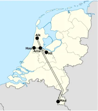
In order to test the methods described in this paper on a real-life application, we constructed a model with m = 7 instances based on actual timetables of the Haarlem-Maastricht (Haa- Maa) and Alkmaar-Hilversum (Alk-Hil) lines of the Dutch Railways and some data provided

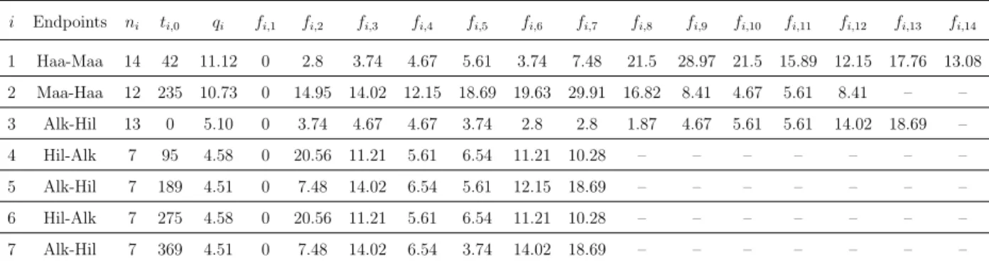
by the railway company, which we extended by a few additional assumptions. The two modeled lines intersect each other in Amsterdam (Ams) at the stations Amsterdam Centraal (Ams-C) and Amsterdam Sloterdijk (Ams-S). Figure 1 is a schematic illustration of the two intersecting lines. The case study contains n = 67 events in total. The parameters of the instances (event counts, initial departure times as minutes after midnight, quantities of distributable supplements and feasible event-to-event times in minutes) are summarized in Table 1.

Figure 1: Map of the Haarlem-Maastricht and Alkmaar-Hilversum lines, intersecting in Amsterdam

The model containsq= 7 interferences for scheduled passenger transfers at these stations as well as rolling stock connections between the endpoint of an instance and the starting point of the following instance in the reverse direction of the same line. The parameters of the interferences (their instance and event indices and prescribed safety margins in minutes) are

Source of image: cUser: Lencer / Wikimedia Commons / CC-BY-SA-3.0, with additional modifications.

Some pairs of oppositely directed instances on identical lines have different event counts as we modeled both express and local trains. Instead of modeling both departures and arrivals at all stops, we only modeled one event per stop (only departures except for arrivals at final stations).

i Endpoints ni ti,0 qi fi,1 fi,2 fi,3 fi,4 fi,5 fi,6 fi,7 fi,8 fi,9 fi,10 fi,11 fi,12 fi,13 fi,14

1 Haa-Maa 14 42 11.12 0 2.8 3.74 4.67 5.61 3.74 7.48 21.5 28.97 21.5 15.89 12.15 17.76 13.08 2 Maa-Haa 12 235 10.73 0 14.95 14.02 12.15 18.69 19.63 29.91 16.82 8.41 4.67 5.61 8.41 – – 3 Alk-Hil 13 0 5.10 0 3.74 4.67 4.67 3.74 2.8 2.8 1.87 4.67 5.61 5.61 14.02 18.69 –

4 Hil-Alk 7 95 4.58 0 20.56 11.21 5.61 6.54 11.21 10.28 – – – – – – –

5 Alk-Hil 7 189 4.51 0 7.48 14.02 6.54 5.61 12.15 18.69 – – – – – – –

6 Hil-Alk 7 275 4.58 0 20.56 11.21 5.61 6.54 11.21 10.28 – – – – – – –

7 Alk-Hil 7 369 4.51 0 7.48 14.02 6.54 3.74 14.02 18.69 – – – – – – –

Table 1: Parameters of the instances summarized in Table 2.

k Station i⁰_k j_k⁰ ik jk sk

1 Ams-C 3 11 1 5 5

2 Ams-S 2 11 7 5 5

3 Maa 1 14 2 1 5

4 Hil 3 13 4 1 5

5 Alk 4 7 5 1 5

6 Hil 5 7 6 1 5

7 Alk 6 7 7 1 5

Table 2: Parameters of the interferences

There are no additional restrictions in the model (r = 0). Before discretization, we assumed the disturbances to be independent right-truncated exponential random variables with orig- inal means µ_i,j = E(˜ω_i,j) given by µ_i,1 = 0.2, µ_i,j = 0.07f_i,j (j > 1) and a truncation threshold of ten minutes: ω_i,j = min(10,ω˜_i,j) (i∈I, j ∈J_i). We assigned (non-normalized) delay weights of zero to initial departures, two to intermediate departures with transfer opportunities (interferences) as well as to final arrivals and one to other intermediate depar- tures, as initial departure delays are largely irrelevant, and the punctuality of transfers and final arrivals has a key importance.

In this example, the sequence of events R_h (h= 1,2, . . . , n) starts as

R₁ = (1,1), R₂ = (1,2), R₃ = (1,3), R₄ = (1,4), R₅ = (3,1), R₆ = (3,2) etc.,

We include truncation in the model following [16] as delays could explode otherwise, whereas the aim of the model is to increase the robustness of timetables against regular relatively small disturbances.

where a switch to the third instance occurs in the fifth term due to the first interference, which prescribes that the fifth event of the first instance has two wait for the eleventh event of the third instance before moving on. For the sake of illustration, we include here some associated delay formulas in recursive form:

y_1,1^∗ (x,ω) = (ω_1,1−x_1,1)⁺,

y_1,2^∗ (x,ω) = (y_1,1^∗ (x,ω) +ω_1,2−x_1,2)⁺, y_1,3^∗ (x,ω) = (y_1,2^∗ (x,ω) +ω_1,3−x_1,3)⁺, y_1,4^∗ (x,ω) = (y_1,3^∗ (x,ω) +ω_1,4−x_1,4)⁺,

y_1,5^∗ (x,ω) = max((y^∗_1,4(x,ω) +ω_1,5−x_1,5)⁺, y^∗_3,11(x,ω)−d₁(x) + 5), . . .

4.1 Numerical solution

We applied statistical sampling from the joint distribution of the disturbances via Monte Carlo simulation, using the resulting empirical distributions in the model instead of the orig- inal exponential distributions. This technique is called external sampling ([28]). Assuming some fairly mild technical conditions, it may be proved that the optimal solution and the optimal objective function value of the approximating problem are strongly consistent sta- tistical estimators of those of the original problem (see [28] for a proof and further properties of the method), so the optimal solution of the sequence of approximating problems with increasing sample sizes converges to the true optimal solution with probability one. Addi- tionally, following [16], we applied the technique ofantithetic variables (see e.g. [25]) in order to increase the precision of the discrete approximation for a given sample size. We solved the problem with several sample sizes, and finally decided to user = 1000 joint realizations, as increasing the sample size only altered the optimal solution negligibly beyond this value.

We solved problem (16) in the model management system SLP-IOR using the Regularized Decomposition algorithm for SP models. Additionally, for the sake of comparison, we also

We define the plus operator asa⁺= max(a,0) (a∈R).

solved the equivalent LP and NLP formulations presented in Section 3 in the computer al- gebra system Maplesoft Maple 2015 ([18]) using a built-in sparse interior point algorithm for the LP and the Sequential Quadratic Programming algorithm for the NLP formulation.

The three algorithms arrived at the same optimal solution with computation times of 33.27 minutes (LP), 1.49 minutes (SP) and 1.06 minutes (NLP). These results indicate that us- ing more advanced formulations instead of solving the equivalent LP as done earlier in the literature (in e.g. [16] and [30]) pays off in terms of computational efficiency, especially for larger models of even more complex real-life networks. In the remainder of our paper, we shall stick to the SP formulation, as we shall focus on non-computational issues.

In addition to the three solution frameworks examined so far, we tested an additional, rather heuristic solution to present evidence that relying on intuition may lead to poor allocations.

A naive analysis might suggest that it provides a fairly good solution to allocate the sup- plements proportionally to the mean disturbances associated with the events, which is often done by railway companies in real-life timetables. In order to test this approach, we fixed the values of the decision variables in the SP model to follow a proportional allocation, which increased the optimal objective function value by 13.0%. This is a highly signifi- cant increase in practice, suggesting that using proportional allocations should be avoided in real-life timetables.

4.2 Analysis of the role of distributional assumptions

Our choice of the exponential distribution was motivated by several previous publications including [6], [16], [30] and [32], which described experiments indicating that observed dis- turbances fit well to exponential distributions. Nevertheless, as a high level of sensitivity of the optimal solution with respect to the chosen distributional form would indicate a low level of practical reliability, it is important to investigate the effect of our choice on the optimal solution. Therefore, in addition to the truncated exponential distributions, we performed a sensitivity analysis using the following distributional assumptions forω_i,j (i∈I, j ∈J_i, with

On a computer with a 2.8 GHz Intel Core i7 processor and 4 GB RAM.

the parameters µ_i,j the same as in Table 1):

• Untruncated exponential with meanµ_i,j,

• Pareto with two degrees of freedom and cdf F_i,j(x) = 1−

µi,j

x+µi,j

2

(x≥0).

• Uniform on (0,2µ_i,j).

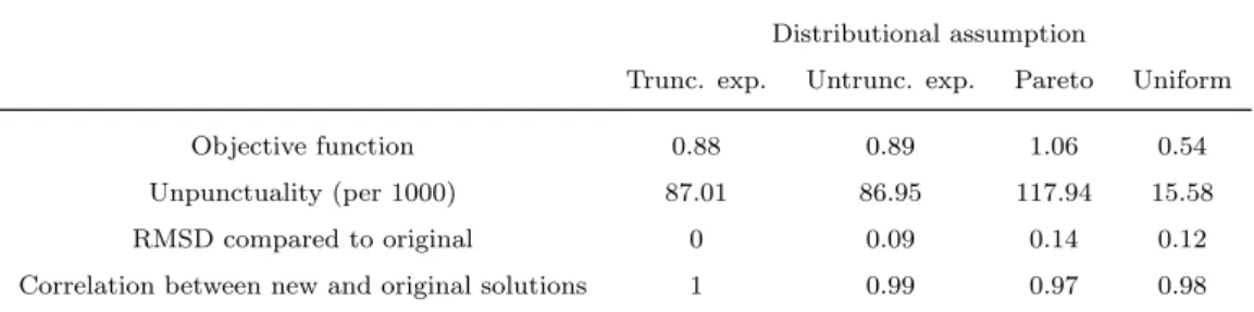
We selected these three distributions in order to test the effects of omitting truncation, introducing heavy tails and a lack of positive skewness, respectively, and calibrated them to have equal means so as to ensure their comparability. We summarize the results of our analysis in Table 3. The results indicate that the lack of truncation and heavy tails increase

Distributional assumption

Trunc. exp. Untrunc. exp. Pareto Uniform

Objective function 0.88 0.89 1.06 0.54

Unpunctuality (per 1000) 87.01 86.95 117.94 15.58

RMSD compared to original 0 0.09 0.14 0.12

Correlation between new and original solutions 1 0.99 0.97 0.98

Table 3: Main results for different disturbance distributions

the mean delay and unpunctuality, whereas the lack of skewness decreases them due to increased predictability. More importantly, the RMSD (root-mean-square difference) and the correlation coefficient of the new and original first-stage solution vectors indicates a very high level of similarity of the optimal solutions of the modified problems to the original one, which implies a high degree of robustness of the optimal solution of our model even if the exponential distribution is not appropriate or truncation is dropped from the model.

4.3 Analysis of the role of the total amount of supplements

As increasing the amount of supplements results in decreased delays at the cost of increased planned travel times, there is a natural trade-off between delays and planned travel times, to be regulated by a reasonable choice of the amount of distributable supplements. For this reason, it is important to analyze whether the actual values of the supplements used by the

Dutch Railways, amounting to 7% of the planned travel times, are reasonable. To address this question, we constructed the following modified version of problem (16):

D= min

x≥0,γ≥0{E_ω[∆(x,ω)] +βM(γ) :

ni

X

j=1

x_i,j ≤γq_i (i∈I), constraints (5) and (13)}

where M(γ) = γ

m

X

i=1 ni

X

j=1

˜

w_i,jq_i and ∆(x,ω) = min

y≥0{wy: constraints (14) and (15)}.

In this modified problem, the total amount of distributable supplements for each instance is scaled by a factor γ > 0, and their weighted mean M(γ) is penalized in the first-stage objective function by a linear term with an exogenous penalty coefficient 0< β <1. Thus the modified first-stage objective function is the sum of the expected weighted mean delay and an additional penalty term, which is the product of a penalty coefficient and the weighted mean of the planned excess travel times arising due to the use of supplements. Here the penalty parameter expresses how many times planned excess times are more undesirable than unexpected delays. It is natural to assume that β < 1, as passengers obviously prefer expected excess times to unexpected ones. Due to the previously explained trade-off between expected and unexpected excess times, the first term is decreasing and the second one is increasing in the scale parameterγ, which implies that there is a value γ^∗ that optimizes the trade-off, and its value depends on the penalty parameter β. Thus by finding the parameter value β^∗ that results in γ^∗ = 1, we may determine which penalty parameter results in the same optimal quantities of distributable supplements as the ones currently used in practice.

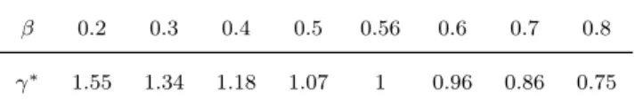
We shall call this valueβ^∗ the implied penalty parameter of the current timetable. We solved the modified problem using different values of the parameter β and recorded the optimal values γ^∗ for each run. The numerical results shown in Table 4 indicate the implied penalty parameter β^∗ ≈ 0.56, or in other words, the current timetable assumes that unexpected excess travel times are somewhat less than twice as undesirable as expected ones.

β 0.2 0.3 0.4 0.5 0.56 0.6 0.7 0.8

γ^∗ 1.55 1.34 1.18 1.07 1 0.96 0.86 0.75

Table 4: Optimal scale parameters for different values of the penalty parameter If e.g. it is more reasonable to assume that unexpected excess travel times areexactly twice

as undesirable as expected ones, than the current values of supplements should be increased by a factor of 1.07 according to Table 4.

4.4 Analysis of the effect of dependent disturbances

As the independence assumption is rather unrealistic, we now investigate the effect of possible dependence among the disturbances. To this end, a parametric multidimensional distribu- tion needs to be fully specified. This is greatly simplified by the use of copulas (see e.g.

[20]), which are cumulative probability distribution functions over the multidimensional unit hypercube, as it is known from Sklar’s theorem (again, see [20]) that any multivariate prob- ability distribution is uniquely determined by the associated marginal distributions and a copula function. Out of several parametric families of copulas that are known in the liter- ature, we propose the n-dimensional Gaussian copula due to its computational tractability.

It is defined asC(z₁, z₂, . . . z_n) = Φ_Rh

Φ⁻¹(z₁),Φ⁻¹(z₂), . . . ,Φ⁻¹(z_n)i

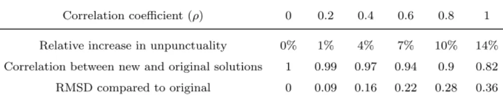
(0< z₁, z₂, . . . , z_n <1), where Φ_R and Φ⁻¹ denote the joint cdf of the n-dimensional standard normal distribution with correlation matrixR and the quantile function (inverse cdf) of the univariate standard normal distribution, respectively. To make our analysis one-dimensional, we used a simple correlation matrix with R_g,h = ρ (g 6= h, g, h ∈ {1,2, . . . , n},0 ≤ ρ ≤ 1) and R_g,g = 1 (g ∈ {1,2, . . . , n}), and solved the original SP problem with the additional assumption of this Gaussian copula joining the disturbances, while leaving their marginal distributions un- changed. In the external sampling algorithm, we sampled from the Gaussian copula using the Cholesky decomposition of the matrixR (this technique is described in [4]).

Our numerical results for different correlation coefficients are summarized in Table 5.

Correlation coefficient (ρ) 0 0.2 0.4 0.6 0.8 1 Relative increase in unpunctuality 0% 1% 4% 7% 10% 14%

Correlation between new and original solutions 1 0.99 0.97 0.94 0.9 0.82 RMSD compared to original 0 0.09 0.16 0.22 0.28 0.36

Table 5: Main results for different levels of dependence

The relative increases in unpunctuality indicate that higher levels of dependence result in