Automatic roundo¤ error analysis of numerical algorithms

(1)

Óbuda University

PhD thesis

Automatic roundo¤ error analysis of numerical algorithms

by

Attila Gáti Supervisors:

Prof. Dr. László Horváth Prof. Dr. István Krómer

Applied Informatics Doctoral School

Budapest, 2013

(2)

1 Introduction

The idea of automatic error analysis of algorithms and/or arithmetic expressions is as old as the scienti…c computing itself and originates from Wilkinson (see Higham [39]), who also developed the theory of ‡oating point error analysis [80], which is the basic of today’s ‡oating point arithmetic standards ([65], [62]). There are various forms of automatic error analysis with usually partial solutions to the problem (see, e.g. Higham [39],[21]). The most impressive approach is the interval analysis, although its use is limited by the technique itself (see. e.g. [59], [60], [61], [43], [44], [76], [39]). Most of the scienti…c algorithms however are implemented in ‡oating point arithmetic and the users are interested in the numerical stability or robustness of these implementations. The theoretical investigations are usually di¢ cult, require special knowledge and they do not always result in conclusions that are acceptable in practice (for the reasons of this, see, e.g. [79], [80], [11], [39], [21]). The common approach is to make a thorough testing on selected test problems and to draw conclusions upon the test results (see, e.g. [69], [70], [77]).

Clearly, these conclusions depend on the "lucky" selection of the test problems and in any case require a huge amount of extra work. The idea of some kind of automatization arised quite early.

The e¤ective tool of linearizing the e¤ects of roundo¤ errors has been widely applied since the middle of the 70’s ([52], [53], [54], [55], [56], [57], [58], [73], [47], [72]). Given a numerical method the computed value is a function R(d; ) (R : R^n+m ! R^k), where d 2 Rⁿ is the input vector, and is the vector of individual relative rounding errors on themarithmetic operations ( 2R^m,k k₁ u, where u is the machine rounding unit). Considering the …rst order Taylor expansion of R at = 0 we have for all j = 1;2; : : : ; k

R_j(d; ) =R_j(d;0) + Xm

i=1

@R_j

@ _i (d;0) +o(k k) (1) From (1) an approximate error bound for the forward error immediately follows:

jR_j(d; ) R_j(d;0)j/ (d)u (j = 1;2; : : : ; k) (2) where

(d) = max

j

Xm i=1

@R_j

@ i

(d;0) (3)

The need for computing the partial derivatives accurately and e¤ectively motivated the design of new automatic di¤erentiation techniques. Since R is given as an algorithm, it is decomposed to basic arithmetic operations and elmentary functions.

By automatic di¤erentiation we apply systematically the chain rule of calculus according to the relation "being an operand of" among the operations and elementary

(4)

functions to compute the derivatives of the composition function R. In contrast to numerical di¤erentiation, automatic di¤erentiation is free of truncation errors.

On the other hand it has the drawback, that we can not treat numerical methods as black boxes, because we need the structural knowledge of their decomposition to basic operations and elementary function. The data structure commonly used to represent the structure of a numerical method is the computational graph.

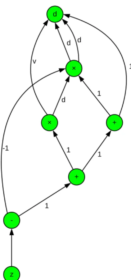
Let us consider a simple example from [53]:

v d d;

w d+v;

x d v;

y w+x;

z y v:

with a single input d, and a single output z. The corresponding computational graph is shown in Figure 1.

Concerning the computational graph related error analysis Chaitin-Chatelin and Frayssé [11] gave the following summary.

"The stability analysis of an algorithm x = G(y) with the implementation G_alg = G⁽ⁱ⁾ depends on the partial derivatives ^@G_@y⁽ⁱ⁾

j computed at the various nodes of the computational graph (see § 2.6). The partial derivatives show how inaccuracies in data and rounding errors at each step are propagated through the computation. The analysis can be conducted in a forward (or bottom-up) mode or a backward (or top-down) mode. There have been several e¤orts to automate this derivation. One can cite the following:

1. Miller and Spooner (1978);

2. the B-analysis: Larson, Pasternak, and Wisniewski (1983), Larson and Sameh (1980);

3. the functional stability analysis: Rowan (1990);

4. the automatic di¤erentiation (AD) techniques:

Rall (1981), Griewank (1989), Iri (1991)"

Miller developed his approach in several papers ([49], [50], [51], [52], [53], [54], [55], [56], [57], [58]). The basic idea of Miller’s method is the following. Given a numerical algorithm to analyze, a number !(d) is associated with each set d (d 2 Rⁿ) of input data. The function ! : Rⁿ ! R measures rounding error, i.e.,

!(d) is large exactly when the algorithm applied to d produces results which are

(5)

d

×

× +

+

-

z

1 d d

v

d 1

-1 1

1

Figure 1: A computational graph.

excessively sensitive to rounding errors. A numerical maximizer is applied to search for large values of ! to provide information about the numerical properties of the algorithm. Finding a large value of ! can be interpreted as the given numerical algorithm is su¤ering from a speci…c kind of instability.

The software performs backward error analysis. The value !(d) u (whereuis the machine rounding unit) can be interpreted as the …rst order approximation of the upper bound for the backward error. The computation of the error measuring number is based on the partial derivatives of the output with respect to the input and the individual rounding errors. An automatic di¤erentiation algorithm is used to provide the necessary derivatives.

The Miller algorithm was implemented in Fortran language (actually in FOR- TRAN IV) by Webb Miller and David Spooner [56], [57] in 1978. More information on the use of the software by Miller and its theoretical background can be found in [52], [53], [54] and [56]. The software is in the ACM TOMS library with serial number 532 [57].

In the book of Miller and Wrathall [58], the potential of the software is clearly

(6)

demonstrated through14case studies. The answers of the software are consistent in these cases with the well known formal analytical and experimental results. The program shows correctly the stability properties of algorithms such as the

inversion of triangular matrices

the linear least-squares problem by solving the normal equations Gaussian elimination without pivoting and with partial pivoting, the Gauss-Jordan elimination,

the Gaussian elimination with iterative improvement, the Cholesky factorization,

Cholesky factorization after rank-one modi…cation, the classical and modi…ed Gram-Schmidt methods,

the application of normal equations and Householder re‡ections for linear least squares problem,

rational QR method, downdating of the QR factorization,

the characteristic polynomial computation by the Faddeev method, symmetric matrix representations.

Miller’s approach was further developed for relative error analysis by Larson, Pasternak, and Wisniewski [47]. Larson et al. [47] say (pp. 125–126) the following.

"To perform the error analysis, the algorithm being analyzed is represented as a directed graph with each numeric quantity being a node in this graph. Directed arcs lead from operands to their results. Each node’s value is subject to error, called local relative error. This error a¤ects those subsequent nodes that are computed using the contamined node as an operand. All of the local relative errors together are used to produce a total relative error for each node. From the directed graph, a system of equations relating to the local and total relative errors is generated.

Our software is related to that of Miller [4] and Miller and Spooner [5], which analyzes the numerical stability of algorithms using absolute error analyses. In particular, the input formats are similar, and the minicompiler, a program for translating a FORTRAN-like language into the data format for the code [5], can be used to specify the computational graph of the algorithm being analyzed."

(7)

Rowan [72] considers the numerical algorithms as black boxes. The two main elements of his approach is a function that estimates a lower bound on the backward error, and a new optimization method (called subplex and based on the Nelder-Mead simplex method) that maximizes the function. A numerical method is considered unstable if the maximization gives a large backward error. The FOR- TRAN software requires two user-supplied Fortran subprograms; one implements the algorithm to be tested in single precision, and the other provides a more accurate solution, typically by executing the same algorithm in double precision.

Bliss [5], Bliss et al [6] developed Fortran preprocessor tools for implementing the local relative error approach of Larson and Sameh. They also used some sta- tistical techniques as well. The structure of their "instrumentation environment"

is shown in Figure 2 taken from Bliss et al [6].

Cedar Fortran Preprocessor

-z pass

Performance Data Flow Numerical Quality

OP_COUNT

Cache Studies

LGRAPH PERTURB

TOMS 594 (Larson)

TOMS 532 (Miller)

Interval analysis Infinite precision arithm.

Qualitative stability

Figure 2: The "instrumentation environment" of Bliss et al [6].

Error analysis tools based on the di¤erential error model have been developed not only for numerical but also for symbolic computing environments. Stoutemyer [73] was the …rst to use computer algebra for error-analysis software. He used the accumulated error expressions from the di¤erential error model to determine a bound on the error and proposes analyzing the condition expressions to …nd points where instability is a problem. For other authors and approaches, see Mutrie et

(8)

al. [63], Krämer [43], [44], or [39].

Finally, we have to mention the PRECISE toolbox of Chaitin–Chatelin et al.

[11], [21] that embodies an entirely di¤erent strategy (somewhat similar to the naive testing, but much more sophisticated). "PRECISE allows experimentation about stability by a straightforward randomisation of selected data, then lets the computer produce a sample of perturbed solutions and associated residuals or a sample of perturbed spectra." ([11], p. 104).

Upon the basis of corresponding literature, the Miller approach seems to be the most advanced although Miller’s method has several setbacks. The numerical method to be analyzed must be expressed in a special, greatly simpli…ed Fortran- like language. We can construct for-loops and if-tests that are based on the values of integer expressions. There is no way of conversion between real and integer types, and no mixed expressions (that contains both integer and real values) are allowed. Hence we can de…ne only straight-line programs, i.e., where the ‡ow of control does not depend on the values of ‡oating point variables. To analyze methods with iterative loops and with branches on ‡oating point values, the possible paths through any comparisons must be treated separately. This can be realized by constrained optimization. We con…ne search for maximum to those input vectors by which the required path of control is realized. The constraints can be speci…ed through a user-de…ned subroutine.

Higham [39] points out that the special language and its restrictions as the greatest disadvantage of the software:

". . .yet the software has apparently not been widely used. This is probably largely due to the inability of the software to analyse algorithms expressed in For- tran, or any other standard language".

Unfortunately, this can be said more or less on the other developments that followed the Miller approach.

The aim of my research work is to improve Miller’s method to a level that meet today’s requirements. I improved and upgraded Miller’s method in two main steps.

The …rst step was a F77 version usable in PC environment with standard F77 compilers such as the GNU and Watcom compilers [24], [25], [26]. This version was able to handle algorithms with a maximum of 3000 inputs, and a maximum of 1000 outputs, and operations of a maximum of 50000 while the original Miller program was able to handle a maximum of 30 inputs, 20 outputs and 300 operations [24], [25], [26]. However even this new version used the simpli…ed Fortran like language of Miller which is considered as a major problem by Higham and others. Using the recently available techniques such as automatic di¤erentiation, object oriented programming and the widespread use of MATLAB, I have eliminated the above mentioned drawbacks of Miller’s method by creating a Matlab interface. Applying

(9)

the operator overloading based implementation technique of automatic di¤erentiation Griewank [37] and Bischof etal [4] we have provided means of analyzing numerical methods given in the form of Matlab m-functions. In our framework, we can de…ne both straight-line programs and methods with iterative loops and arbitrary branches. Since the possible control paths are handled automatically, iterative methods and methods with pivoting techniques can also be analyzed in a convenient way. Miller originally used the direct search method of Rosenbrock for …nding numerical instability. To improve the e¢ ciency of maximizing, we added two more direct search methods [30], [28], [29], [35]: the well known simplex method of Nelder and Mead, and the so called multidirectional search method developed by Torczon [75].

In the thesis we present a signi…cantly improved and partially reconstructed Miller method by designing and developing a new Matlab package for automatic roundo¤ error analysis. Our software provides all the functionalities of the work by Miller and extends its applicability to such numerical algorithms that were complicated or even impossible to analyze with Miller’s method before. Since the analyzed numerical algorithm can be given in the form of a Matlab m-…le, our software is easy to use.

We used the software package to examine the stability of some ABS methods [1], [2], namely the implicit LU methods and several variants of the Huang method [25]. The obtained computational results agreed with the already known facts about the numerical stability of the ABS algorithms. The program has shown that implicit LU is numerically unstable and that the modi…ed Huang method has better stability properties than the original Huang method and the famous MGS (modi…ed Gram-Schmidt) method (see [58], [2] or [36]).

We also tested three fast matrix multiplication algorithms with the following results:

1. The classical Winograd scalar product based matrix multiplication algorithm of O(n³) operation cost is highly unstable in accordance with the common belief, that has never been published.

2. Both the Strassen and Winograd recursive matrix multiplication algorithms of O(n^2:81) operation costs are numerically unstable.

3. The comparative testing indicates that the numerical stability of Strassen’s algorithm is somewhat better than those of Winograd.

Upon the basis of our testing, we may think that the new software called Miller Analyzer for Matlab will be useful for numerical people or algorithm developers to analyze the e¤ects of rounding errors. The results of my research were published in the works [24], [25], [26], [27], [30], [28], [29], [31], [32], [33], [34], [35].

(10)

2 The original Miller-Spooner software and its limitations

Using the software, the numerical method to analyse must be expressed in a special and simpli…ed Fortran-like language. The language allows the usage of integer and real types. The variables can be scalars, or one or two dimensional arrays of both types. We can construct for-loops and if tests, but only that are not based on the values of real variables. This means, that we can only de…ne algorithms, in which the ‡ow of control does not depend on the value of ‡oating point variables. To analyse methods that contain branching based on the value of real variables the possible pathes through comparisions have to be treated separately. This can be realized by constrained optimization. We constrain the search for maximum to such input vectors, by which the required path of control is realized. The constraints can be speci…ed through a user-de…ned Fortran subroutine, called POSITV.

The software package consists of three programs, a minicompiler and two error analyser programs. The minicompiler takes as data the numerical method to analyse, written in a special programming language, and produces as output a translation of that program into a series of assignment statements. The output is presented in a readable form for the user, and in a coded form for use as input to the error analyser programs. One of the error analyser programs (i) is for deciding numerical stability of a single algorithm, and the other (ii) is for comparing two algorithms. The input for the error-testing programs is arranged as follows: (1) the output of the minicompiler (For program (i), it is the compiled version of the algorithm to analyse. In the case of program (ii) we must provide the compiled version of the two algorithms to compare), (2) a list of initial data for the numerical maximizer, (3) the code of the chosen error-measuring value, (4) target value for the maximizer. The programs return with the …nal set of data found by the maximizer routine and with the value of the chosen error-measuring number at this set of data.

If program (i) diagnoses instability (the value of the error-measuring number at the …nal set of data exceeds the target value) then the condition number is also computed at the …nal set of data.

The minicompiler does its job in two phases: the compilation phase and the interpreter-like execution phase. In the compilation phase the program makes syntactical and semantical analysis, and generates an intermediate code (a coded representation of the algorithm to analyse) for the interpreter routine. The interpreter executes this intermediate code in a special way. All integer expressions are actually evaluated in order to perform the correct number of iterations of for-loops, and to interpretively perform if-then tests. In contrast no actual real arithmetic computation is done. The interpreter does not evaluate the ‡oating point operations, only registers them in the form of assignment statements. Throughout all

(11)

real variables are treated symbolically as being the n-th input value, intermediate value, or real constant. The restrictions of the language ensures, that the pro- duced series of assignment statements, which is actually a representation of the algorithms computational graph, is independent from the input data. Based on the computational graph generated by the minicompiler, the error analyser programs compute the partial derivatives of the output of the analyzed numerical method with respect to the inputs and individual rounding errors in every data required by the maximizer routine. The di¤erentiation is realized through graph algorithms, so the applied method is not numerical derivation. The computation of stability measuring function is based on these partial derivatives. The direct search method used for maximizing is the Rosenbrock method.

The Miller-Spooner roundo¤ error analyser software was written in Fortran IV for the IBM 360/370 series, and its …nal version were issued in 1979, which can be downloaded from the NETLIB repository. Without any modi…cations, it can not be used in a PC environment with the most widely used compilers based on the Fortran 77 standard (GNU compiler, Watcom, Lahey, etc.), because there are several non-standard solutions in the source. By compilation we get several error messages, but even if we are able to correctly eliminate these errors we get a program, which simply does not work. The semantical problems are arising from two facts. First, the software uses EBCDIC character encoding instead of ASCII.

Second, the correct working of the program requires, that some local variables be static i.e., they have to keep their values between two function or procedure calls.

Unlike in older Fortran dialects this is not guaranteed by the Fortran 77 standard.

In addition, the original version bounds the user to extraordinary strict limitations in the size of the algorithm to analyse. The number of inputs cannot exceed 30, the number of outputs must be smaller than 20, and the total number of inputs and real arithmetic operations may not exceed 300. The limits are due to small values of constants determining the sizes of static arrays used in the software.

Another weak point of the sofware is maximizing, because it can be done only by direct search, as the function ! is not di¤erentiable. Direct search methods are heuristic, so sometimes the program can provide misleading results. Failure of the maximizer to …nd large values of ! does not guarentee that none exists. The method tends to be optimistic: unstable methods may appear to be stable.

Finally, we have to note that the software is rather inconvenient to use. The input stream for the error analyser programs must be made out by hand. If we want to perform constrained optimization through the POSITV routine, we have to relink the program, and the method of analysing algorithms containing branching based on the values of real variables by constrained optimization can be rather complicated in some cases.

The original Miller program can handle a maximum of 30 inputs, 20 outputs

(12)

and 300 operations. My F77 variant of Miller’s algorithm can handle algorithms with a maximum of 3000 inputs, 1000 outputs, and 50000 arithmetic operations [25].

3 Straight-line programs, computational graphs and automatic di¤erentiation

Miller’s error analyzer treats rounding errors in a machine independent manner.

The analysis is not tuned to a particular form of machine number or a particular numerical precision, instead it employs a model of ‡oating point numbers and rounding errors. We use the standard model of the ‡oating point arithmetic, which assumes that the relative error of each arithmetic operation is bounded by the machine rounding unit, and we ignore the possibility of over‡ow and under‡ow.

The IEEE 754/1985 standard of ‡oating point arithmetic guarantees that the standard model holds for addition, subtraction, multiplication, division and square root (see, e.g. Muller et al. [62]). Unfortunately it is not true for the exponential, trigonometric, hyperbolic functions and their inverses. Hence we limit ourselves to numerical algorithms that can be decomposed to the above mentioned …ve basic operations and unary minus, which is considered error-free.

The roundo¤ error analyzer method of Miller is based on the …rst order derivatives of the output with respect to the input and the belonging rounding errors.

Our main improvement concerns the automatic di¤erentiation method computing the values for the Jacobian. In order to describe the applied techniques precisely, we need to make clear the concepts of a straight-line program and a computational graph and their role in the applied automatic di¤erentiation method.

First, we introduce the notion of a straight-line program. Informally, a numerical algorithm is a straight-line program if it does not contain branches depending directly or indirectly on the particular input values, and the loops are traversed a

…xed number of times. With the loops unrolled, taking the appropriate branches at if-tests and inlining the subroutines — i.e., inserting the content of a subroutine in the place of its call — , one could create an equivalent program containing only sequence of real assignment statements to every straight-line program. By de…ning straight-line programs and computational graphs, we follow Castano et al. [10] with slight modi…cations.

Now we give the formal de…nition of a straight-line program . Let m, n and t be natural numbers and introduce X = fx₁; x₂; : : : ; x_ng, V = fv₁; v₂; : : : ; v_mg and f ;+; ; ; ;sqrtg disjoint sets of n, m and six symbols, respectively, and let S = fs₁; s₂; : : : ; s_tg be a set of t real numbers. We shall call the elements of S constants, the elements ofX inputs and the elements ofV intermediate results

(13)

of the straight-line program . A computational sequence C is an m-tuple with elements of the form v v⁰ v⁰⁰ or v sqrtv⁰ or v v⁰ (1 m, 2 f+; ; ; g), wherev⁰ andv⁰⁰are either elements ofV with lower index than , or arbitrary elements of the setS[X. A straight-line program of lengthmwith n inputs, t constants and k outputs is an ordered quintuple = (S; X; V; T; C), whereS R, andX,V are disjoint sets of symbols as above witht,n,melements, respectively. T is a subset of V with cardinality k, and C is a computational sequence of length m. The elements of T are the outputs of the straight-line program .

An interpretation of the straight-line program in the domainRof real numbers is a mappingJ :X !R. If J can be extended to a mappingS[X[V !R (for convenience also denoted byJ) in such a way that J(s) =s for every s2S, and for every1 m the identity

J(v ) = 8<

:

J(v⁰) J(v⁰⁰) if c =v v⁰ v⁰⁰ pJ(v⁰) if c =v sqrtv⁰

J(v⁰) if c =v v⁰

(4) de…ned and holds, then we call the interpretationconsistent (c denotes the entry of C with index ). It is obvious that there exists at most one consistent way to extend a given mappingJ, and such an extension exists unless we encounter values for which any of the prescribed operations are unde…ned (attempting to division by zero or taking the square root of a negative number). A consistent interpretation on R gives rise to a …nite sequence of real numbers: J(x₁), J(x₂); : : : ; J(x_n), J(v1), J(v2); : : : ; J(vm). The numbers di = J(xi) are the actual input values, and w_j = J(v_j) are called intermediate values. If T = fv_j₁; v_j₂; : : : ; v_j_kg, then the interpretation results k outputs p₁ = w_j₁, p₂ = w_j₂, : : :, p_k = w_j_k. We also say that the interpretation computes the outputs p1; p2; : : : ; pk from the inputs d₁; d₂; : : : ; d_n.

Let = (S; X; V; T; C)be a straight line program. We associate to a labeled directed acyclic graph G( ) whose set of nodes is S [ X [V. The elements of S [X represent nodes that are not the starting point of any edges, and the corresponding elements of S[X will also be the label of these nodes. The nodes labeled by elements of S are called constant nodes whereas the nodes labeled by elements ofX are called input nodes. The elements of the setV are the arithmetic nodes of G. If v v⁰ v⁰⁰ is an element of the computational sequenceC, then G contains two edges from the node v to v⁰ and v⁰⁰, and the node v is labeled by . Analogously, if c is of the form of v sqrtv⁰ orv v⁰ an edge goes from v to v⁰, and v is labeled by sqrt and , respectively. Finally we add k additional nodes (output nodes) labeled by the elements ofT. Gcontains an edge from each output node to the arithmetic node giving the value of that output. We call G( ) the computational graph associated to the straight-line program .

(14)

A given computational graph may be associated to di¤erent straight-line programs, which however compute all the same outputs. Hence from now on, we consider the straight-line program and its computational graph equivalent.

We de…ne the program function of the straight-line program on domain R as follows. Let D be the set of all vectors d 2 Rⁿ for which the corresponding interpretation J(x_i) = d_i, (i = 1;2; : : : ; n) is consistent. For every d 2 D the consistent interpretation computes the output vector p2 R^k resulting a function P :D!R^k. This mapping will be called the program function of the straight-line program on domain R.

Let = (S; X; V; T; C) be a straight-line program as above, and let 2 R^m be the vector of rounding errors hitting each operation in C. The standard model of ‡oating point arithmetic guarantees that j ^jj u for all j = 1;2; : : : ; m, where u is small positive number, the machine rounding unit. An interpretation of the straight-line program on the domain R in the presence of error vector is a mapping J :X ! R. If J can be extended to a mapping Jb:S [X[V ! R in such a way that Jb(s) = s for every s2S, and for every 1 m the identity

Jb(v ) = 8>

><

>>

:

Jb(v⁰) Jb(v⁰⁰) (1 + ) if c =v v⁰ v⁰⁰ qJb(v⁰) (1 + ) if c =v sqrtv⁰

Jb(v⁰) if c =v v⁰

(5)

de…ned and holds, then we call the interpretationconsistent.

Let Db be the set of all pairs (d; ) of vectors d 2 Rⁿ, 2 R^m for which the corresponding interpretation J(x_i) = d_i (i = 1;2; : : : ; n) is consistent in the presence of rounding errors . For every (d; ) 2 Db the consistent interpretation computes the output vectorpb2R^k resulting a functionR :Db !R^k, the program function of the straight-line program on domainRwith presence of rounding errors.

It is obvious that for alld2D, (d;0)2Db also holds, and P(d) = R(d;0).

The analysis of the e¤ects of rounding errors on the evaluation ofP atd₀ 2D in ‡oating point arithmetic according to the computational sequenceCis based on the derivatives ofRat(d₀;0)2Db with respect to the entries ofdand . According to the straight-line program representation and equation (5), the function R is decomposed into the composition of' (1 m) elementary functions. For all 1 m ' has the form:

' (x; y; ") = (x y) (1 +") if c =v v⁰ v⁰⁰ ' (z; ") = p

z(1 +") if c =v sqrtv⁰

' (x) = x if c =v v⁰

where x; y; z; " 2 R, z 0, j"j u. The required derivatives of R are evaluated by automatic (sometimes also called algorithmic) di¤erentiation techniques, i.e.,

(15)

knowing the elementary functions and their derivatives, we apply systematically the chain rule of calculus according to the dependence relation given by the computational graph to build the derivatives of the composition functionR. The applied automatic di¤erentiation algorithm requires the di¤erentiability of the elementary functions. Thus we have to restrict the domains of the functionsP andRto ensure that no square root of zero will be encountered in (4) and (5) (except the case ofv⁰ being a constant, which is not a practical implementation ofP). LetJ :X!Rbe a consistent interpretation of the straight-line program in the domainR. We call the interpretation di¤erentiable if for every entry of the computational sequence of C with the form v sqrtv⁰ the corresponding identity J(v ) = p

J(v⁰) holds with J(v⁰)>0.

4 Numerical stability measures

The numerical stability measures used in Miller’s algorithm were developed by Miller in a sequence of papers [49], [51], [54], [56] and [58]. The purpose of this chapter is to give an understanding of how the software measures the e¤ects of rounding errors, and how the error measuring function is formulated. Actually we can perform analysis based on several error measuring numbers (various ways of assigning !), and beside analysing the propagation of rounding errors in a single algorithm we can also compare the numerical stability of two competiting numerical methods, which neglecting rounding errors compute the same values.

The method treats rounding errors in a machine independent manner. The analysis is not tuned to a particular form of machine number or a particular numerical precision, instead it employs a model of rounding errors. The applied model is the standard model of the ‡oating point arithmetic, which assumes that the relative error of each arithmetic operation is bounded by the machine rounding unit, and we ignore the possibility of over‡ow and under‡ow. The allowed arithmetic operations are addition, substraction, multiplication, division, square root and unary minus, but unary minus is always considered to be error free.

First let us consider the case of analysing a single algorithm. The software provides four stability-measuring numbers, J W_E(d), J W_L(d), W K_E(d), W K_L(d), which measure the minimum problem perturbation equivalent to rounding error in a given program at data d. Other numbers ERE(d) and ERL(d) use weaker comparison of computed and exact solutions. To give the precise de…n- ition of these error measuring functions we shall need some notations. Suppose that S Rⁿ, T S and f : S ! R^m. Notation f(T) will denote the set:

f(T) = ff(t)2R^m :t2Tg. We extend some operations on vectors to sets of vectors: let S; S₁; S₂ Rⁿ, v 2Rⁿ be a vector, 2R a scalar and A2 R^{m n} an

(16)

m by n matrix, then the sets S, AS, v+S,S₁+S₂ will be de…ned as:

S = f x:x2Sg AS = fAx:x2Sg v+S = fv+x:x2Sg

S₁+S₂ = fx+y :x2S₁; y 2S₂g.

Suppose R is a numerical algorithm applying only the allowed arithmetic operations mentioned above. If the operations are performed in ‡oating point arithmetic, with the assumption of the standard model, then the computed value is a function R(d; ) (R : R^n+m ! R^k), where d 2 Rⁿ is the input vector, and is the vector of individual relative rounding errors on the m arithmetic operations ( 2 R^m, k k₁ u, where u is the machine rounding unit). Let f = R(d;0) be the exact solution. K⁽ⁿ⁾ = fx 2 Rⁿ : kxk₁ 1g will denote the maximum norm unit ball. For all d 2 S D_E(d) = diag(d) will be a diagonal matrix with d_i as its i-th diagonal entry, andD_L(d) =diag(kdk₁)will stand for a diagonal matrix with the largest entry of the input vector as all of its diagonal elements. We similarly de…ne diagonal matrices for the exact result: F_E =diag(f(d)), andF_L =diag(kf(d)k₁).

Using these notations we can de…ne the stability measuring numbers as follows:

J W_E(d) = inf 0 :R(d; uK^(m)) f(d+ uD_EK⁽ⁿ⁾) J W_L(d) = inf 0 :R(d; uK^(m)) f(d+ uD_LK⁽ⁿ⁾)

W K_E(d) = inf 0 :R(d; uK^(m)) f(d+ uD_EK⁽ⁿ⁾) + uF_EuK^(k) W KL(d) = inf 0 :R(d; uK^(m)) f(d+ DLuK⁽ⁿ⁾) + uFLK^(k)

ER_E(d) = inf 0 : R(d; uK^(m)) f(d)

1 f(d+ uD_EK⁽ⁿ⁾) f(d)

1

ERL(d) = inf 0 : R(d; uK^(m)) f(d)

1 f(d+ uDLK⁽ⁿ⁾) f(d)

1 . In the de…nitions R(d; uK^(m)) is the set of possible computed values under the assumption of the standard model of ‡oating point arithmetic. On the right-hand side of the subset sign in the de…nitions we have compact sets, which implies that the in…mums are achieved. So we can say that for any 2 R^m; k k₁ u, there exists a vector 2 Rⁿ, j ⁱj J W_E(d) jd_ij u (i = 1;2; : : : ; n) for which R(d; ) =f(d+ ) holds, and J W_E(d) is the smallest such number. This means thatJ WE(d) uis the least upper bound for the componentwise relative backward error. Analogous fact holds forJ W_L(d)with the relationj ⁱj J W_L(d) kdk₁ u (i = 1;2; : : : ; n) for the vector , so J W_L(d) u is the least upper bound for the normwise relative backword error. In the case of the W KX measures (X =E, or L) we also allow perturbations in the output space. For any 2 R^m; k k₁ u, there exist a vector 2Rⁿ, j ⁱj W K_E(d) jd_ij u (i= 1;2; : : : ; n)and a vector

(17)

'2R^kj'_ij W K_E(d) jf_i(d)j u(i= 1;2; : : : ; k)for whichR(d; ) =f(d+ )+' holds and W KE(d) is the least such number. So W KE(d) u can be interpreted as the least upper bound for the relative mixed forward-backward error measured componentwise. As the same is true for W K_L(d) with j ⁱj W K_L(d) kdk₁ u (i= 1;2; : : : ; n)and j'_ij W KL(d) kf(d)k₁ u(i= 1;2; : : : ; k), W KL(d)is the least upper bound for the normwise relative mixed forward-backward error. Notice that the relations W K_L(d) W K_E(d) J W_E(d) and W K_L(d) J W_L(d) J WE(d)will hold.

The numbersJ W_X andW K_X require that the computed solution be obtained at (or close to) exact solution. ER_X measures how much the data must be perturbed to create an error as large as that in the computed solution. In the case of ER_E it is true, that for any 2 R^m; k k₁ u, there exists a vector 2 Rⁿ, j ⁱj ER_E(d) jd_ij u (i = 1;2; : : : ; n) for which kR(d; ) f(d)k₁ = kf(d+ ) f(d)k₁ holds, and ERE(d) is the least such number. The same is true forER_L(d)with the relationj ⁱj ER_L(d) kdk₁ u(i= 1;2; : : : ; n)for the vector . The inequalities ER_L(d) ER_E(d) and ER_X (d) J W_X(d) (X =E, orL) are obvious.

Now let us take a glance at the error-measuring numbers used to compare the stability properties of two algorithms. Let Q and R be two algorithms for evaluating the function f; and the computed values at data d, with rounding errors 2R^land 2R^m be denoted byQ(d; )and R(d; ). The error measuring functions are de…ned as:

J W_R=Q = inf 0 :R(d; uK^(m)) Q(d; uK^(l)) ER_R=Q = inf 0 : R(d; uK^(m)) f(d)

1 Q(d; uK^(l)) f(d)

1 : We can say, that for any 2 R^m; k k₁ u, there exists a vector 2 R^l, j ij J W_R=Q(d) u (i = 1;2; : : : ; n) for which R(d; ) = Q(d; ) holds, and J W_R=Q(d)is the smallest such number. Regarding the standard model of machine arithmetic the computed values given byRcan be achived with rounding errors in Qbounded byJ W_R=Q(d) u:In the case ofER_R=Q it is true, that for any 2R^m; k k₁ u, there exists a vector 2 R^l, j ij ER_R=Q(d) u (i = 1;2; : : : ; n) for which kR(d; ) f(d)k₁ = kQ(d; ) f(d)k₁ holds, and ER_R=Q(d) is the smallest such number. ER_R=Q u can be interpreted as the least upper bound for the relative roundo¤ errors in Q, by which Q produces output with as large forward error as does R in ‡oating point arithmetic with machine rounding unit u. The inequalities ER_Q=R(d) J W_Q=R(d) and ^{J W}

Q X

J W_X^R J W_Q=R(d) (X = E, or L) will also hold.

The software gives …rst order approximation of the above error measuring numbers based on the partial derivatives of R with respect to the input vectord and the individual rounding errors , or in the case of comparing two algorithms the

(18)

derivatives of Q and R with respect to rounding errors. The desired derivatives are obtained by automatic di¤erentiation on the computational graph of the given numerical algorithm(s).

5 The optimization algorithms

In order to achieve global error bounds Miller’s algorithm applies a numerical maximizer routine. Since in general the error measuring functions are not di¤erentiable, a direct search method, the method of Rosenbrock [71] is used. Naturally, it is not guaranteed that global maximum is reached, since the maximizer routine may terminate in a local extremum, or it is also possible that it fails to converge at all. So sometimes we may get misleading results: unstable methods may appear to be stable. On the other hand the various error measuring numbers have the adventage, that the relations holding among them usually prevents the user to accept missleading results. Since the publication of Rosenbrock’s method, the derivative-free optimization has also developed a lot (see, e.g. [64], [75], [45], [9], [48], [42], [13], [23]). In order to improve the performance of the program I selected, programmed and tested two extra methods. These are the famous Nelder-Mead simplex method ([64], [45], [9], [48], [42], [13], [23]) and Torczon’s multidirectional search ([75], [48], [42], [13]). The two selected algorithms are the following:

The Nelder-Mead method

Initialization: Choose an initial simplex of vertices Y₀ =fy₀⁰; y₀¹; : : : ; yⁿ₀g. Evaluate f at the points in Y₀. Choose constants:

0< y^s<1; 1< îc<0< ôc< ^r < ê: Fork = 0;1;2; : : :

0. Set Y =Y_k.

1. Order: Order the n+ 1 vertices ofY =fy⁰; y¹; : : : ; yⁿgso that f⁰ =f y⁰ f¹ =f y¹ fⁿ =f(yⁿ):

2. Re‡ect: Re‡ect the worst vertexyⁿ over the centroid y^c =Pn 1 i=0 yⁱ=n of the remaining n vertices:

y^r =y^c+ ^r(y^c yⁿ):

Evaluatef^r =f(y^r). Iff⁰ f^r < fⁿ ¹, then replaceyⁿby the re‡ected point y^r and terminate the iteration: Y_k+1 =fy⁰; y¹; :::; yⁿ ¹; y^rg. 3. Expand: Iff^r< f⁰, then calculate the expansion point

y^e =y^c + ^e(y^c yⁿ)

(19)

and evaluatefê =f(yê). If fê f^r, replace yⁿ by the expansion point yê and terminate the iteration: Yk+1 =fy⁰; y¹; :::; yⁿ ¹; yêg. Otherwise, replaceyⁿ by the re‡ected pointy^r and terminate the iteration:

Y_k+1 =fy⁰; y¹; :::; yⁿ ¹; y^rg:

4. Contract: If f^r fⁿ ¹, then a contraction is performed between the best ofy^r and yⁿ.

(a)Outside contraction: If f^r < fⁿ, perform an outside contraction y^oc=y^c+ ^oc(y^c yⁿ)

and evaluate fôc =f(yôc). If fôc f^r , then replace yⁿ by the outside contraction pointyôc_k and terminate the iteration:

Y_k+1 =fy⁰; y¹; :::; yⁿ ¹; y^ocg: Otherwise, perform a shrink.

(b)Inside contraction: If f^r fⁿ, perform an inside contraction y^ic=y^c+ ^ic(y^c yⁿ)

and evaluate fîc =f(yîc). If fîc < fⁿ, then replace yⁿ by the inside contraction point yîc and terminate the iteration:

Y_k+1 =fy⁰; y¹; :::; yⁿ ¹; y^icg: Otherwise, perform a shrink.

5. Shrink: Evaluate f at then pointsy⁰+ ^s(yⁱ y⁰), i= 1; : : : ; n, and replacey¹; :::; yⁿ by these points, terminating the iteration:

Y_k+1 =fy⁰+ ^s(yⁱ y⁰); i= 0; :::; ng: The MDS method

Initialization: Choose an initial simplex of vertices Y₀ =fy₀⁰; y₀¹; : : : ; yⁿ₀g. Evaluate f at the points in Y₀. Choose constants:

0< ^s<1< ^e: Fork = 0;1;2; :::

0. Set Y =Yk.

1. Find best vertex: Order the n+ 1 vertices of Y =fy⁰; y¹; :::; yⁿg so that f⁰ =f(y⁰) f(yⁱ), i= 1; :::; n:

(20)

2. Rotate: Rotate the simplex around the best vertex y⁰: y_i^r =y⁰ (yⁱ y⁰); i= 1; :::; n:

Evaluate f(y^r_i), i= 1; :::; n, and setf^r= minff(y_i^r) :i= 1; :::; ng. If f^r < f⁰, then attempt an expansion (and then take the best of the rotated or expanded simplices). Otherwise, contract the simplex.

3. Expand: Expand the rotated simplex:

y_i^e=y⁰ ^e(yⁱ y⁰); i= 1; :::; n:

Evaluate f(yê_i),i= 1; :::; n, and setfê = minff(y_iê) :i= 1; :::; ng. Iffê< f^r, then accept the expanded simplex and terminate the iteration: Yk+1 =fy⁰; yê₁; :::; yê_ng. Otherwise, accept the rotated simplex and terminate the iteration: Y_k+1 =fy⁰; y₁^r; :::; y_n^rg.

4. Shrink: Evaluate f at then pointsy⁰+ ^s(yⁱ y⁰), i= 1; :::; n, and replacey¹; :::; yⁿ by these points, terminating the iteration:

Y_k+1 =fy⁰+ ^s(yⁱ y⁰); i= 0; :::; ng:

Details on the convergence and implementation may be found in the literature [71], [64], [75], [45], [9], [48], [42], [13], [23].

5.1 Comparative testing of the applied direct search meth- ods

In the following, I give some test results about the use of the applied direct search methods. The tests concern three algorithms, also discussed by Miller in his case studies [58]: inversion of triangular matrices using back substitution, Gaussian elimination without pivoting and Gauss-Jordan elimination with partial pivoting.

We consider such error functions in each test case that are known to be unbounded (see Miller [58]), and we investigate the number of function evaluations required by the direct search methods to reach the target value of10000. The size parameter for the matrix to invert and the system of equitions to solve by the Gauss and Gauss-Jordan elimination methods will be set to n= 4,n = 8 and n= 16 in each case.

(21)

5.1.1 Triangular matrix inversion

Table 1 shows the results for the analysis of inverting triangular matrices using back substitution. We started the maximizer routines from the diagonal matrix

D= 2 66 66 64

1 2

3 . ..

n 3 77 77 75 .

In this case, the Multidirectional search method was the only method that could n Rosenbrock Nelder-Mead Multidirectional

4 232

8 184

16 680

Table 1: Number of function evaluations required to maximize the normwise backward error for triangular matrix inversion.

…nd a value greater than10000 for the normwise backward error (J WL).

5.1.2 Gaussian elimination

The results for Gaussian elimination are shown in Table 2. The error function to maximize was the normwise mixed forward-backward error (W KL). The maximization was started from the system:

A = 2 66 66 64

3 1 1 1

1 4 1 1

1 1 5 1

... ... ... . .. ...

1 1 1 n+ 2

3 77 77 75

; b=

2 66 66 64

n+ 2 n+ 3 n+ 4

... 2n+ 1

3 77 77 75

. (6)

Table 3 shows the results of a test that was the same as the previous except we constrained the maximization to symmetric matrices. The search was started fom (6).

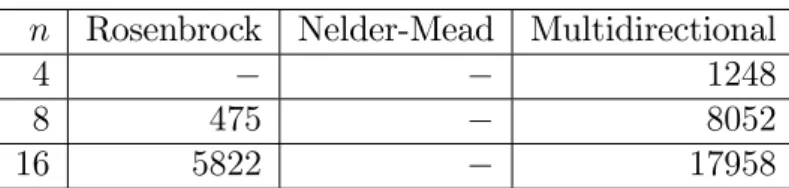
5.1.3 Gauss-Jordan elimination with partial pivoting

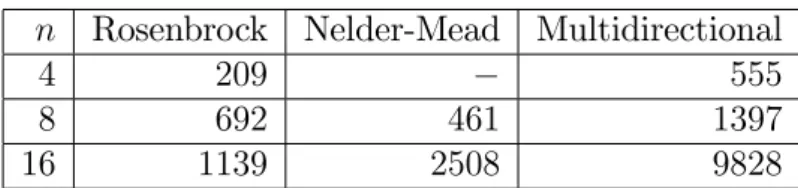
Finally, I have tested the search methods on the normwise backward error (J WL) for Gauss-Jordan elimination with partial pivoting. The results are shown in Table 4. The Nelder-Mead simplex method failed for all sizes.

(22)

n Rosenbrock Nelder-Mead Multidirectional

4 209 555

8 692 461 1397

16 1139 2508 9828

Table 2: Number of function evaluations required to maximize the normwise mixed forward-backward error for Gaussian elimination.

4 162 324

8 226 1631

16 1843 759 3195

Table 3: Number of function evaluations required to maximize the normwise mixed forward-backward error for Gaussian elimination. The search was constrained to symmetric matrices.

From the above examples one could deduce that the less robust method is the Nelder-Mead simplex method. As the multidirectional search method found the target value in all cases it is our strongest method, but it requires much more function evaluations and so computational time, than the other two methods. A good practice could be if we start an analysis using the Rosenbrock method, and if it fails we can exploit multidirectional search.

6 The new operator overloading based approach of di¤erentiation

Now, we brie‡y discuss the technique of automatic di¤erentiation that we have applied in our software. To fully understand this section, the reader should be familiar with the object oriented concept of operator overloading and the way it can be used to implement automatic di¤erentiation tools. For the required information please consult Rall [67] or Griewank [37].

The original software by Miller has its own programming language. The analyzed numerical algorithm must be expressed in that simpli…ed, Fortran-like language. The restrictions of the language guarantee that the de…ned program can be converted to an equivalent formal straight-line program. A software module called the minicompiler compiles the given algorithm into a straight-line program as the …rst step of analysis.

The problem is that programs containing iterative loops that may be traversed variable number of times and branches that modify calculation according to various

(23)

4 1248

8 475 8052

16 5822 17958

Table 4: Number of function evaluations required to maximize the normwise backward error for Gauss-Jordan elimination.

criteria cannot be handled by the Miller’s minicompiler. On the other hand the straight-line program and the computational graph is still an accurate model of such a program as it is executed upon a given …xed d input vector. Loops can be unrolled, and only certain branches of the program are actually taken in each given case. By executing any numerical program, we can record the arithmetic operations occurred in the form of a computational sequence as an execution trace of all the operations and their arguments. With the nomination of the input and output variables, we get a straight-line program, for which the derivatives can be calculated in the same way as by Miller’s original approach. Of course, for di¤erent input data we may get di¤erent straight-line programs by tracing the execution.

Let d2Rⁿ be a vector of input data upon which a given numerical algorithm can be executed without any arithmetic exceptions and run-time errors. Tracing the execution we get a straight-line program d= (S_d; X; V_d; T_d; C_d)with program functions Pd in exact arithmetic and Rd in the presence of rounding error. Under our assumptions the interpretation J(x_i) = d_i, (i = 1;2; : : : n) will be consistent, and if it is also di¤erentiable, then we can calculate the Jacobian of function R_d at(d;0)2R^n+m^d.

The basic idea of operator overloading approach of automatic di¤erentiation is that we use a special user de…ned class instead of the built-in ‡oating point type, for which all the arithmetic operators and the square root function are de…ned (overloaded). Upon performing the operations on the variables of that special type, in addition to computing the ‡oating point result of the operation, the appropriate entry (node) is also added to the computational sequence (graph). Such a class must contain at least two …elds (data members): the actual ‡oating point value as in the case of ordinary variables and an identi…er that identi…es the entry (node) in the computational sequence (graph) corresponding to the given ‡oating point value.

We have developed a Matlab interface for automatic di¤erentiation, which over- loads the arithmetic operators and the functionsqrt for Matlab vectors and matrices of class real (complex arithmetic is not supported). By executing the m-…le code of the analyzed numerical algorithm using our special class instead of class real, we get the required computational sequence as a trace of execution. Our approach is much the same as the overloaded automatic di¤erentiation libraries

(24)

ADMAT (developed by Coleman and Verma [12], Verma [78] and MAD (by Shaun A. Forth [22]). The main di¤erence is that unlike these toolboxes we also calculate the partial derivatives with respect to the rounding errors in addition to the derivatives with respect to the inputs.

7 The Miller Analyzer for Matlab

Miller Analyzer for Matlab is a mixed-language software. We kept several routines from the work of Miller et al. [57], which was written in Fortran.

These routines perform automatic di¤erentiation using graph techniques on the computational graph, compute error measuring numbers from the derivatives and do the maximization of the error function. The interface between Matlab and the Fortran routines is implemented in C++. The source has to be compiled into a Matlab MEX …le, and it is to be called from the command prompt of Matlab. The integration into the Matlab environment makes the use of the program convenient.

Matlab provides an easy way of interchanging vectors and matrices with the error analyzer software, and we can immediately verify the results either by testing the analyzed numerical method or by applying some kind of a posteriori roundo¤

analysis upon the …nal set of data returned by the maximizer.

Applying the operator overloading technology of Matlab (version 5.0 and above, for details see Register [68]), we have provided a much more ‡exible way of de…ning the numerical method to analyze, than the minicompiler did. This new way is based on a user-de…ned Matlab class calledcfloating, on which we have de…ned all the arithmetic operators and the function sqrt. The functions de…ning these operators compute the given arithmetic operations and create an execution trace of the operations as a computational sequence. To analyze a numerical method, we can implement it in the form of Matlab m-…le using cfloatingtype instead of the built-in ‡oating point type. However, the cfloating class can do more then the original compiler (the minicompiler of Miller) since it does not only register the

‡oating point operations, but also computes their results. During execution the value of real variables are available, which through the overloading of relational operators makes it possible to de…ne numerical methods containing branches based on values of real variables and iterative loops (i.e., algorithms that are not straight- line).

Still, this is not yet enough to analyze the numerical stability of such algorithms, because unlike the minicompiler the generated computational graph may depend on the input data. Algorithm 1 gives the high level pseudocode of the original program of Miller. Statements (1) and (2) are performed by the minicompiler. As the analyzed method is guaranteed to be straight-line, the generated computational graph is independent from the ‡oating point input vector. The

(25)

Algorithm 1The original algorithm 1: Compilation

2: Generating the computational graph 3: repeat

4: for data d required by the maximizer 5: Computing partial derivatives

6: Evaluating of!(d)

7: until(stopping criterion of the maximizer)

Algorithm 2The new approach 1: repeat

2: for data d required by the maximizer 3: Generating the computational graph 4: Computing partial derivatives

5: Evaluating of!(d)

6: until(stopping criterion of the maximizer)

loop given in statements (3)-(7) is executed by the error analyzer program. The program computes the partial derivatives and the stability measuring number for everydinput set of data required by the maximizer. The program terminates if the stopping criterion of the numerical maximizer is ful…lled. Algorithm 2 illustrates our new approach. In this case the compilation phase is omitted since the Matlab interpreter executes the m-…le directly. The problem is that the generated computational graph is not necessarily independent from the input data. Therefore, the process that builds the computational graph had to be inserted into the main loop (Algorithm 2, statement (3)). In this way our program is able to analyze the numerical stability of algorithms that are not straight-line.

7.1 De…ning the numerical method to analyse by m-…le programming

The numerical method to analyse must be implemented in a special way in the form of m-functions. The numerical algorithm can be given either as a single m-function, or it can be organized into a main m-function and one or more subfunctions. The purpose of these m-…les is to build the computational graph corresponding to the

‡oating point operations performed when the numerical algorithm is executed upon a given input data. Instead of the built-in double precision MATLAB array, we use a special class called c‡oating, for which the arithmetic operators and the function

(26)

sqrt for square root are de…ned (overloaded). When the error analyser calls the main m-function, the MATLAB interpreter executes it. Upon performing the operations on the variables of type c‡oating, beside computing the ‡oating point result of the operation, the appropriate node is also added to the computational graph. The c‡oating class contains two …elds (data members): the actual ‡oating point value, as in the case of ordinary variables, and a node identi…er, which identi…es the node in the graph corresponding to the given ‡oating point value.

As every MATLAB variable, c‡oating is also an array, and every element of the array contain the two …elds: value and node identi…er. It can be a matrix (two dimensional array) or a multidimensional array (array with more than two dimension). Scalars (1-by-1 array) and vectors (1-by-n or n-by-1 array) are special matrices in MATLAB. The MATLAB operators: +; ; ; =; : ; :=; :n and the function sqrt can be applied, scalar, vector, and matrix operations are also supported. The c‡oating type substitutes the real, double precision MATLAB type, the complex arithmetic is not supported directly. By algorithms involving complex computation, the user must decompose the complex operations to real arithmetic by hand. We are planning to add direct support of complex arithmetic in the future.

7.1.1 The main m-function Algorithm 3Main function

1: function main( identi…er )

2: identi…er=miller_ptr(identi…er);

3: Initializing the input as c‡oating arrays and adding the input nodes to the graph 4: Run the algorithm using c‡oating type

to add the arithmetic nodes

and compute the output as c‡oating array 5: Add the output nodes to the graph

end

The main m-function is the m-function that is dedicated to be called by the error analyser, when the computational graph has to be built. Algorithm 3 shows the general form of the main m-function. As in line 1, the main m-function must have one input argument and it must not have any output arguments. To make

(27)

MATLAB able to …nd our main m-function, it has to be reside in an m-…le with the same name, and the m-…le must be on the MATLAB path or in the working directory. Line 2 ful…lls a formal requirement, all such m-functions have to be begun with that statement. Actually it creates a handle to the computational graph being built and we will use it for several purposes (instead of ’identifier’

any valid variable name can be used).

In our model the analysed numerical method computes a function P (d) (P : Rⁿ!R^k,d2Rⁿ is the input vector) The lengthn of the input vectordis always

…xed for analysis, error maximization is performed in then dimensional space Rⁿ. In many cases P is not de…ned at every point in Rⁿ, since no division by zero may occur and no square root of a negative number may be taken. If the MATLAB interpreter encounters such an operation, it signals the error condition by throwing an exception. The maximizer catches the error, so the maximization process is not terminated, but continues at other datad.

We say that a numerical algorithm is a straight-line program, if it does not contain branches depending directly or indirectly on the particular input values, and the loops are all unrollable taxative loops. In the case of such programs a unique computational graph represents the algorithm (assuming that the number of inputs is …xed), so it is enough to call the main m-function and build the computational graph only once¹. On the other hand, if the ‡ow of control depends on the input values, we regenerate the graph by calling the main function at every d input data, upon which the error measuring number is to be computed. In such cases, the number of arithmetic operations may also depend on d:

In a computational graph, there can be four kinds of node. First we add the input nodes that correspond to the n entries of the input vector d (see line 3).

In the next step (line 4) we run the algorithm on d. Beside evaluating the m operations, we also addmarithmetic nodes to the graph. We distinguish six kinds of arithmetic nodes: four correspond to the binary operations (+, -, *, /) and two to square root and unary minus. A constant value may also appear as operand in an operation. In the graph, constant nodes corresponds to the constant values used in the algorithm. Finally, some of the arithmetic nodes are designated as output nodes meaning that the result of the given operation is one of the output values of the algorithm (line 5). In order to evaluate the error measuring number at d, the partial derivatives of the values corresponding to the output nodes with respect to the values corresponding to the input nodes and the relative rounding errors hitting the arithmetic nodes will be computed.

1In some cases we run the algorithm at the …rst time in order to count the operations and determine the amount of memory to allocate, and make an additional call to build the graph.