Hexagonal parallel thinning algorithms based on sufficient conditions for topology preservation
P´eter Kardos & K´alm´an Pal´agyi
Department of Image Processing and Computer Graphics, University of Szeged, Szeged, Hungary
Thinning is a well-known technique for producing skeleton-like shape features from digital binary objects in a topology preserving way. Most of the existing thinning algorithms presuppose that the input images are sampled on orthogonal grids. This paper presents new sufficient conditions for topology preserving reductions working on hexagonal grids (or triangular lattices) and eight new 2D hexagonal parallel thinning algorithms that are based on our conditions. The proposed algorithms are capable of producing both medial lines and topological kernels as well.
1 INTRODUCTION
Various applications of image processing and pat- tern recognition are based on the concept of skele- tons (Siddiqi and Pizer 2008). Thinning is an itera- tive object reduction until only the skeletons of the bi- nary objects are left (Lam et al. 1992; Suen and Wang 1994). Thinning algorithms in 2D serve for extract- ing medial lines and topological kernels (Hall et al.
1996). A topological kernel is a minimal set of points that is topologically equivalent to the original object (Hall et al. 1996; Kong and Rosenfeld 1989; Kong 1995; Ronse 1988). Some thinning algorithms work- ing on hexagonal grids have been proposed (Deutsch 1970; Deutsch 1972; Staunton 1996; Staunton 1999;
Wiederhold and Morales 2008; Kardos and Pal´agyi 2011)
Parallel thinning algorithms are composed of re- duction operators (i.e., some object points having value of “1” in a binary picture that satisfy certain topological and geometric constrains are changed to
“0” ones simultaneously) (Hall 1996).
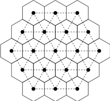
Digital pictures on non–orthogonal grids have been studied by a number of authors (Kong and Rosen- feld 1989; Marchand-Maillet and Sharaiha 2000). A hexagonal grid, which is formed by a tessellation of regular hexagons, corresponds, by duality, to the tri- angular lattice, where the points are the centers of that hexagons, see Figure 1. The advantage of hexagonal grids over the orthogonal ones lies in the fact that in hexagonal sampling scheme, each pixel is surrounded by six equidistant nearest neighbors, which results in a less ambiguous connectivity structure and in a
Figure 1: A hexagonal grid and the corresponding tri- angular lattice
better angular resolution compared to the rectangular case (Lee and Jayanthi 2005; Marchand-Maillet and Sharaiha 2000).
Topology preservation is an essential requirement for thinning algorithms (Kong and Rosenfeld 1989).
In order to verify that a reduction preserves topol- ogy, Ronse and Kong gave some sufficient conditions for reduction operators working on the orthogonal grid (Kong 1995; Ronse 1988), then later, Kardos and Pal´agyi proposed similar conditions for the hexagonal case, that can be used to verify the topological cor- rectness of the thinning process (Kardos and Pal´agyi 2011).
In this paper we present some new alternative suffi- cient conditions for topology preservation on hexago- nal grids that make possible to generate deletion con- ditions for various thinning algorithms and we also introduce such algorithms based on these conditions.
The rest of this paper is organized as follows. Sec-
p p4
p1
p6 p3 p2
p5
Figure 2: Indexing scheme for the elements ofN6(p) on hexagonal grid. Pixelspi (i= 4,5,6), for whichp precedespi, are gray dotted.
tion 2 reviews the basic notions of 2D digital hexag- onal topology and some sufficient conditions for re- duction operators to preserve topology. Section 3 dis- cusses the proposed hexagonal parallel thinning al- gorithms that are based on the three parallel thin- ning schemes. Section 4 presents some examples of the produced skeleton-like shape features. Finally, we round off the paper with some concluding remarks.
2 BASIC NOTIONS AND RESULTS
Let us consider a hexagonal grid denoted by H, and let pbe a pixel in H. Let us denote N6(p) the set of pixels being 6-adjacent to pixel p and let N6∗(p) = N6(p)\{p}.Figure 2 shows the 6–neighbors of a pixel pdenoted byN6(p). The pixel denoted bypi is called as thei-th neighborof the central pixelp. We say that pprecedesthe pixelsp4, p5, andp6. (It is easy to see that the relation “precedes” is irreflexive, antisymmet- ric, and transitive, therefore, it is a partial order on the setN6(p).)
The sequence S of distinct pixels hx0, x1, . . . , xni is called a 6-path of lengthn from pixel x0 to pixel xn in a non-empty set of pixels X if each pixel of the sequence is inX andxi is6-adjacent toxi−1 (i= 1, . . . , n). Note that a single pixel is a6-path of length 0. Two pixels are said to be 6-connected in set X if there is a6-path inXbetween them.
Based on the concept of digital pictures as re- viewed in (Kong and Rosenfeld 1989) we define the 2D binary (6,6) digital picture as a quadruple P = (H,6,6, B). The elements ofH are called thepixels ofP. Each element in B ⊆H is called ablack pixel and has a value of 1. Each member ofH\B is called a white pixel and the value of 0 is assigned to it.
6-adjacency is associated with both black and white pixels. An object is a maximal 6-connected set of black pixels, while a white component is a maximal 6-connected set of white pixels. A set composed of three mutually 6-adjacent black pixels p, q, and r is a unit triangle (see Fig. 3). Pixel pis called the first elementof a unit triangle (see Fig. 3).
A black pixel is called a border pixel in a (6,6) picture if it is 6-adjacent to at least one white pixel.
A black pixelpis called and-border pixelin a(6,6)
q r p
r q p
Figure 3: The two possible kinds of unit triangles.
Since p precedes q and q precedes r, pixel p is the first element of the unit triangle.
picture if itsd-th neighbor (denoted bypdin Fig. 2) is a white pixel (d= 1, . . . ,6).
A reduction operator transforms a binary picture only by changing some black pixels to white ones (which is referred to as the deletion of 1’s). A 2D reduction operator doesnotpreserve topology (Kong 1995) if any object is split or is completely deleted, any white component is merged with another white component, or a new white component is created.
Asimple pixel is a black pixel whose deletion is a topology preserving reduction (Kong and Rosenfeld 1989). A useful characterization of simple pixels on (6,6) pictures is stated as follows:
Theorem 1. (Kardos and Pal´agyi 2011)Black pixelp in picture(H,6,6, B)is simple if and only if both of the following conditions are satisfied:
1. pis a border pixel.
2. Picture (H,6,6, N6∗(p) ∩B) contains exactly one object.
Note that the simplicity of pixelpin a(6,6)picture is a local property; it can be decided in view ofN6∗(p).
Reduction operators delete a set of black pixels and not only a single simple pixel. Kardos and Pal´agyi gave the following sufficient conditions for topology preserving reduction operators on hexagonal grids (Kardos and Pal´agyi 2011):
Theorem 2. A reduction operatorOis topology pre- serving in picture (H,6,6, B), if all of the following conditions hold:
1. Only simple pixels are deleted byO.
2. If O deletes two 6-adjacent pixels p, q, then p is simple in (H,6,6, B\{q}), or q is simple in (H,6,6, B\{p}).
3. O does not delete completely any object con- tained in a unit triangle.
While the above result states conditions for pixel- configurations, we can derive from Theorem 2 some new criteria that examine if an individual pixel is deletable or not:
Theorem 3. A reduction operatorOis topology pre- serving in picture(H,6,6, B), if each pixelpdeleted byOsatisfies the following conditions:
1. pis a simple pixel in(H,6,6, B).
2. For any simple pixel q ∈ N6∗(p) preceded by p, pis simple in (H,6,6, B\{q}), orq is simple in (H,6,6, B\{p}).
3. pis not the first element of any object that forms a unit triangle.
Proof. Condition 1 of Theorem 3 corresponds to Condition 1 of Theorem 2. Furthermore, it is obvious that ifpfulfills Condition 2 of Theorem 3 for a given q ∈N6∗(p)but the set {p, q} does not satisfy Condi- tion 2 of Theorem 2, then q must precede p, and as the relation “precedes” is a partial order, this implies thatq is not deleted byO. We show that Condition 3 of Theorem 2 also holds. O does not delete a single pixel object by Condition 1. Objects composed by two 6-adjacent black pixels may not be completely deleted by Condition 2. Finally, from Condition 3 of Theorem 3 follows that exactly one element of any object com- posed by 3 mutually 6-adjacent pixels is retained by O.
Therefore,Osatisfies all conditions of Theorem 3.
Besides the topological correctness, another key re- quirement of thinning is shape preservation. For this aim, thinning algorithms usually apply reduction op- erators that do not delete so-called end pixels that pro- vide important geometrical information related to the shape of objects. We say that none of the black pixels areend pixels of typeE0 in any picture, while a black pixelpis called anend pixel of typeE1 in a(6,6)pic- ture if it is 6-adjacent to exactly one black pixel. Using end pixel characterizationE0leads to algorithms that extract topological kernels of objects, while criterion E1can be applied for producing medial lines.
3 HEXAGONAL THINNING ALGORITHMS In this section, eight thinning algorithms on hexago- nal grids composed of reduction operations satisfying Theorem 3 are reported.
3.1 Fully parallel algorithms
In fully parallel algorithms, the same reduction oper- ation is applied in each iteration step (Hall 1996).
Algorithm 1 introduces the general scheme of our two fully parallel algorithms H-FP-E0and H-FP-E1.
H-FP-ε-deletable pixels (ε∈ {E0, E1}) are defined as follows:
Algorithm 1Algorithm H-FP-ε
1: Input: picture (H, 6, 6, X )
2: Output: picture (H, 6, 6, Y )
3: Y = X
4: repeat
5: D={p|pis H-FP-ε-deletable in Y}
6: Y = Y\D
7: until D=∅
Definition 1. Black pixel pis H-FP-ε-deletable(ε∈ {E0, E1})if it is not anε-end pixel and all the con- ditions of Theorem 3 hold.
The topological correctness of the above algorithm can be easily shown.
Theorem 4. Both algorithms H-FP-E0 and H-FP- E1are topology preserving.
Proof. It can readily be seen that deletable pixels of the proposed two fully parallel algorithms (see Defi- nition 1) are derived directly from conditions of The- orem 3. Hence, both algorithms preserve the topol- ogy.
3.2 Subiteration-based algorithms
The general idea of the subiteration-based approach (often referred to as directional strategy) is that an it- eration step is divided into some successive reduction operations according to the major deletion directions.
The deletion rules of the given reductions are deter- mined by the actual direction (Hall 1996).
For the hexagonal case, here we propose our two 6-subiteration algorithms H-SI-ε(ε∈ {E0, E1}) sketched in Algorithm 2. In each of its subiterations only d-border pixels (d= 1, . . . ,6, see Definition 2) are deleted.
Algorithm 2Algorithm H-SI-ε
1: Input: picture (H, 6, 6, X )
2: Output: picture (H, 6, 6, Y )
3: Y = X
4: repeat
5: D=∅
6: ford= 1to6do
7: Dd={p|pis H-SI-d-ε-deletable in Y}
8: Y = Y\Dd
9: D=D∪Dd
10: end for
11: until D=∅
Here we give the following definition for deletable pixels:
Definition 2. Black pixelpisH-SI-d-ε-deletable(ε∈ {E0, E1}, d= 1, . . . ,6)if all of the following condi- tions hold:
1. p is a simple but not anε-end pixel and it is an d-border pixel in picture(H,6,6, B).
2. If ε=E0, then pis not the first element of any object{p, q}, whereqis ad-border pixel.
Again, we can use Theorem 3 to prove the follow- ing result:
Theorem 5. Algorithms H-SI-E0 and H-SI-E1 are topology preserving.
Proof. If the conditions of Theorem 3 hold for every pixel deleted by our subiteration-based algorithms, then they are topology preserving by Theorem 3. Let pbe a deletedd-border pixel(d= 1, . . . ,6)that does not satisfy the mentioned conditions. Condition 1 of Definition 2 corresponds to Condition 1 of Theo- rem 3. Furthermore, if Condition 2 of Definition 2 holds, then so does Condition 2 of Theorem 3. Con- sequently, p must be the first element of an object {p, q, r} that forms a unit triangle. However, it can be easily seen that in this case, q or r is not a d- border pixel, which means that the object {p, q, r}
may not completely removed by the algorithm. This shows that, even if Condition 3 of Theorem 3 is not fulfilled, algorithms H-SI-E0and H-SI-E1are topol- ogy preserving.
3.3 Subfield-based algorithms
In subfield-based parallel thinning the digital space is decomposed into several subfields. During an itera- tion step, the subfields are alternatively activated, and only pixels in the active subfield may be deleted (Hall 1996). To reduce the noise sensitivity and the num- ber of unwanted side branches in the produced me- dial lines, a modified subfield-based thinning scheme with iteration-level endpoint checking was proposed (N´emeth et al. 2010; N´emeth and Pal´agyi 2011). It takes the endpoints into consideration at the begin- ning of iteration steps, instead of preserving them in each parallel reduction as it is accustomed in the con- ventional subfield-based thinning algorithms.
We propose two possible partitionings of the hexagonal gridHinto three and four subfieldsSFk(i) (k= 3,4; i= 0,1, . . . , k−1)(see Fig. 4).
We would like to emphasize a useful straightfor- ward property of these partitionings:
Proposition 1. Ifp∈SFk(i), thenN6∗(p)∩SFk(i) =
∅(k = 3,4; i= 0, . . . , k−1).
Using these partitionings, we can formulate our four subfield-based algorithms H-SF-k-ε (ε ∈ {E0, E1},k∈ {3,4}) (see Algorithm 3).
SF-k-i-deletable pixels are defined as follows:
1 0 2
0 2 1 0
2 1 0 2 1
0 2 1 0
1 0 2
0 1 0
3 2 3 2
0 1 0 1 0
2 3 2 3
0 1 0
a b
Figure 4: Partitions of H into three (a) and four (b) subfields. For thek-subfield case the pixels markedi are inSFk(i) (k = 3,4; i= 0,1, . . . , k−1)
Algorithm 3Algorithm H-SF-k-ε
1: Input: picture (H, 6, 6, X )
2: Output: picture (H, 6, 6, Y )
3: Y = X
4: repeat
5: D=∅
6: E={p|pis a border pixel but not an end pixel of typeεin Y}
7: fori= 0tok−1do
8: Di={p|p∈Eandpis H-SF-k-i-deletable in Y}
9: Y = Y\Di
10: D=D∪Di
11: end for
12: until D=∅
Definition 3. A black pixel p is H-SF-k-i-deletable in picture(H,6,6, Y)if p is a simple pixel, andp∈ SFk(i) (k∈ {3,4}, i= 0, . . . , k−1).
Now, let us discuss the topological correctness of algorithm H-SF-k-ε(ε∈ {E0, E1},k∈ {3,4}).
Theorem 6. Algorithm H-SF-k-εis topology preserv- ing(ε∈ {E0, E1},k∈ {3,4}).
Proof. By Definition 3, the removal of SF-k-i- deletable pixels satisfies Condition 1 of Theorem 3.
Proposition 1 implies that if p ∈ Di, then N6∗(p)∩ Di = ∅. Consequently, the antecedent of Condition 2 of Theorem 3 never holds, while Condition 3 is always satisfied in the case of algorithms H-SF-k-ε.
Therefore, all the four subfield-based algorithms are topology preserving by Theorem 3.
4 RESULTS
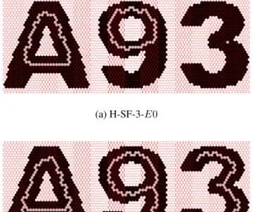
In experiments the proposed algorithms were tested on objects of various images. Due to the lack of space, here we can only present the results for one picture containing three characters, see Figures 5-8, where the extracted skeleton-like shape features are super- imposed on the original objects.
(a) H-FP-E0
(b) H-FP-E1
Figure 5: Topological kernels (a) and medial lines (b) produced by the new fully parallel hexagonal thinning algorithms.
(a) H-SI-E0
(b) H-SI-E1
Figure 6: Topological kernels (a) and medial lines (b) produced by the new subiteration-based hexago- nal thinning algorithms.
(a) H-SF-3-E0
(b) H-SF-3-E1
Figure 7: Topological kernels (a) and medial lines (b) produced by the new 3-subfield hexagonal thinning algorithms.
(a) H-SF-4-E0
(b) H-SF-4-E1
Figure 8: Topological kernels (a) and medial lines (b) produced by the new 4-subfield hexagonal thinning algorithms.
To summarize the properties of the presented algo- rithms, we state the followings:
• All the eight algorithms are different from each other (see Figs. 4-7).
• The four algorithms H-FP-E0, H-SI-E0, H-SF- 3-E0, and H-SF-4-E0 produce topological ker- nels (i.e., there is no simple point in their results).
• Medial lines produced by the four algorithms H- FP-E1, H-SI-E1, H-SF-3-E1, and H-SF-4-E1 are minimal (i.e., they do not contain any sim- ple point except the endpoints of typeE1).
5 CONCLUSIONS
In this work some new sufficient conditions for topol- ogy preserving parallel reduction operations working on (6,6) pictures have been proposed. Based on this result, eight variations of hexagonal parallel thinning algorithms have been reported for producing topolog- ical kernels and medial lines. All of the proposed al- gorithms are proved to be topologically correct.
ACKNOWLEDGEMENTS
This research was supported by the European Union and the European Regional Development Fund under the grant agreements T ´AMOP-4.2.1/B-09/1/KONV- 2010-0005 and T ´AMOP-4.2.2/B-10/1-201-0012, and the grant CNK80370 of the National Office for Re- search and Technology (NKTH) & the Hungarian Sci- entific Research Fund (OTKA).
REFERENCES
Deutsch, E. S. (1970). On parallel operations on hexag- onal arrays. IEEE Transactions on Computers C- 19(10), 982–983.
Deutsch, E. S. (1972). Thinning algorithms on rectan- gular, hexagonal, and triangular arrays. Communi- cations of the ACM 15(9), 827–837.
Hall, R. W. (1996). Parallel connectivity-preserving thinning algorithms. In T. Y. Kong and A. Rosen- feld (Eds.),Topological Algorithms for Digital Im- age Processing, pp. 145–179. New York, NY, USA:
Elsevier Science Inc.
Hall, R. W., T. Y. Kong, and A. Rosenfeld (1996).
Shrinking binary images. In T. Y. Kong and A. Rosenfeld (Eds.), Topological Algorithms for Digital Image Processing, pp. 31–98. New York, NY, USA: Elsevier Science Inc.
Kardos, P. and K. Pal´agyi (2011). On topology preser- vation for hexagonal parallel thinning algorithms. In Proceedings of the International Workshop on Com- binatorial Image Analysis, Volume 6636 ofLecture
Notes in Computer Science, pp. 31–42. Springer Verlag.
Kong, T. Y. (1995). On topology preservation in 2-d and 3-d thinning.IJPRAI 9(5), 813–844.
Kong, T. Y. and A. Rosenfeld (1989). Digital topology:
introduction and survey.Comput. Vision Graph. Im- age Process. 48, 357–393.
Lam, L., S. Lee, and C. Suen (1992). Thin- ning methodologies-a comprehensive survey.IEEE Transactions on Pattern Analysis and Machine In- telligence 14, 869–885.
Lee, M. and S. Jayanthi (2005).Hexagonal Image Pro- cessing: A Practical Approach (Advances in Pattern Recognition). Secaucus, NJ, USA: Springer-Verlag New York, Inc.
Marchand-Maillet, S. and Y. M. Sharaiha (2000). Bi- nary digital image processing - a discrete approach.
Academic Press.
N´emeth, G., P. Kardos, and K. Pal´agyi (2010). Topol- ogy preserving 3d thinning algorithms using four and eight subfields. InProceedings of International Conference on Image Analysis and Recognition, Volume 6111 of Lecture Notes in Computer Sci- ence, pp. 316–325. Springer Verlag.
N´emeth, G. and K. Pal´agyi (2011). Topology preserving parallel thinning algorithms.International Journal of Imaging Systems and Technology 21, 37–44.
Ronse, C. (1988). Minimal test patterns for connectiv- ity preservation in parallel thinning algorithms for binary digital images.Discrete Applied Mathemat- ics 21(1), 67 – 79.
Siddiqi, K. and S. Pizer (2008). Medial Representa- tions: Mathematics, Algorithms and Applications (1st ed.). Springer Publishing Company, Incorpo- rated.
Staunton, R. (1996). An analysis of hexagonal thinning algorithms and skeletal shape representation.PR 29, 1131–1146.
Staunton, R. (1999). A one pass parallel hexagonal thin- ning algorithm. In Image Processing and Its Ap- plications, 1999. Seventh International Conference on (Conf. Publ. No. 465), Volume 2, pp. 841 –845 vol.2.
Suen, C. Y. and P. Wang (1994). Thinning Methodolo- gies for Pattern Recognition. River Edge, NJ, USA:
World Scientific Publishing Co., Inc.
Wiederhold, P. and S. Morales (2008). Thinning on quadratic, triangular, and hexagonal cell complexes.
InIWCIA’08, pp. 13–25.