Topology Preservation and Thinning

(1)

Topology Preservation and Thinning

K´ alm´ an Pal´ agyi

Department of Image Processing and Computer Graphics Institute of Informatics, University of Szeged, Hungary

Dissertation for the Doctoral Degree of the Hungarian Academy of Sciences

2019

(2)

(3)

Preface

The two principal application areas of digital image processing are improve- ment of visual information for human interpretation, and processing of image data for autonomous computer vision. The generic model of a modular computer vision system comprises of image acquisition, preprocessing (i.e., image restoration and enhancement), segmentation (i.e., subdividing an image into its objects), object or shape representation (i.e., extracting shape features from segments), classification and/or interpretation. In this dissertation, our attention is focussed on shape representation, particularly computationally efficient extraction of ‘reliable’ (i.e., geometrically and topologically correct) skeleton-like features from 2D and 3D objects.

Skeletonization (i.e., extracting skeleton-like features from discrete objects in a topology-preserving ways) goes back to Blum’s suggestion. He defined the skeleton (i.e., a region-based shape feature of a continuous object) via the medial axis transform. There is a fairly general agreement that skeletonization procedures play a key role in a broad range of problems in image processing and computer vision.

Digital topology deals with the ‘topological’ nature (particularly, properties of 2D and 3D objects that involve the concept of connectedness, but do not depend on size or shape), and with algorithms that compute or preserve such properties. The importance of topological properties and algorithms show an upward tendency in the analysis of 2D and 3D digital images.

This dissertation presents a selection of my results concerning digital topology, topology-preserving thinning (i.e., a skeletonization technique), and a complex medical application of one of my 3D thinning algorithms. The results included in this work all originate from a period well after defending my PhD dissertation in the year 2000.

The introductory chapter (i.e., Chapter 1) presents the underlying results, and reviews the most important applications of skeletonization. It is followed by three chapters (i.e., Chapters 2–4) that summarize my results.

Chapter 2 reviews some theoretical results concerning diversified topological problems. These results were achieved by the author and P´eter Kardos (i.e., the author’s former PhD student and colleague now). Note that the reported results are absolutely not autotelic, they provide methods of verifying that an operator preserves the topology, allow us to generate topology- preserving operators, and provide computationally efficient thinning algorithms.

(4)

In Chapter 3, only some selected results concerning thinning are presented. The collaborators were my former PhD students and colleagues now:

Péter Kardos and Gábor Németh. This chapter presents a computationally efficient general implementation scheme for thinning algorithms, a safe technique for designing topology-preserving parallel thinning algorithms, four pairs of equivalent sequential and parallel 3D subiteration-based surface- thinning algorithms, and two maximal sequential 3D curve-thinning algorithms.

Chapter 4 describes our complex method for quantitative analysis of pulmonary airway trees that is based on one of the author’s 3D curve-thinning algorithm. Among others, the collaborators were Eric A. Hoffman and Milan Sonka (i.e., outstanding researchers at The University of Iowa, Iowa City, IA, USA).

(5)

To my beloved wife and to the memory of Attila Kuba

(6)

(7)

Acknowledgements

The results reviewed in this dissertation could not have been achieved without the contributions of the coauthors: Emese Balogh (Univ. of Szeged), Kenneth C. Beck (The Univ. of Iowa, Iowa City, IA, USA), Reinhard Beichel (Graz Univ. of Technology, Austria), Horst Bischof (Graz Univ. of Technol- ogy, Austria), Alexander Bornik (Graz Univ. of Technology, Austria), Deok- iee Chon (The Univ. of Iowa, Iowa City, IA, USA), Bal´azs Erd˝ohelyi (Univ.

of Szeged), Attila Fazekas (Univ. of Debrecen), Gerhard Friedrich (Univ. Hos- pital Graz, Austria), Bernhard Geiger (Siemens Corporate Research Prince- ton Inc., Princeton, NJ, USA), Junfeng Guo (The Univ. of Iowa, Iowa City, IA, USA), Csongor Halmai (Univ. of Szeged), Klaus Hausegger (Univ. Hos- pital Graz, Austria), Eric A. Hoffman (The Univ. of Iowa, Iowa City, IA, USA), Christian Janko (Graz Univ. of Technology, Austria), Péter Kardos (Univ. of Szeged), Karl Kiesler (Univ. Hospital Graz, Austria), Domagoj Kovacevic (Univ. of Zagreb, Croatia), György Kovács (Univ. of Debrecen), Attila Kuba (Univ. of Szeged), Franz Lindbichler (Univ. Hospital Graz, Aus- tria), Sven Loncaric (Univ. of Zagreb, Croatia), László Martonossy (Univ.

of Szeged), Brian Matejek (Harvard Univ., Cambridge, MA, USA), Darius Mohadjer (Medical Univ. of Graz, Austria), Geoffrey McLennan (The Univ.

of Iowa, Iowa City, IA, USA), Gábor Németh (Univ. of Szeged), László G.

Nyúl (Univ. of Szeged), Krisztián Ollé (Univ. of Szeged), Hanspeter Pfis- ter (Harvard Univ., Cambridge, MA, USA), Thomas Pock (Graz Univ. of Technology, Austria), Joseph M. Reinhardt (The Univ. of Iowa, Iowa City, IA, USA), Bernhard Reitinger (Graz Univ. of Technology, Austria), Andrea Ruppert (Univ. Hospital Graz, Austria), László Ruskó (Univ. of Szeged), Osama Saba (The Univ. of Iowa, Iowa City, IA, USA), Shaher Samrah (The Univ. of Iowa, Iowa City, IA, USA), Hidenori Shikata (The Univ. of Iowa, Iowa City, IA, USA), Brett A. Simon (The Johns Hopkins Univ., Balti- more, MD, USA), Milan Sonka (The Univ. of Iowa, Iowa City, IA, USA), Erich Sorantin (Univ. Hospital Graz, Austria), Marco Subasic (Univ. of Zag- reb, Croatia), Juerg Tschirren (The Univ. of Iowa, Iowa City, IA, USA), Anna Vilanova i Bartrol´ı (Vienna Univ. of Technology, Austria), Xueying Wang (Harvard Univ., Cambridge, MA, USA), Donglai Wei (Harvard Univ., Cambridge, MA, USA), Georg Werkgartner (Univ. Hospital Graz, Austria), Jinglin Zhao (Harvard Univ., Cambridge, MA, USA), Roman Zotter (Graz Univ. of Technology, Austria).

I gratefully acknowledge their support.

(8)

(9)

Chapter 1 Introduction

This chapter reviews the fundamental concepts and surveys the major theoretical results that we need later on.

Section 1.1 discusses the basic concepts of digital topology including discrete grids, adjacency relations in regular planar grids and the 3D cubic grid, and binary digital pictures.

Section 1.2 surveys sufficient conditions to prove that an algorithm (or an operator) preserves the topology for all possible pictures.

Lastly, in Section 1.3, we review the skeleton of a continuous object, the skeleton-like features to be extracted from 2D and 3D digital objects, the major skeletonization techniques, and the applications of skeletonization.

(12)

1.1 Basic Concepts of Digital Topology

Digital topology deals with the topological properties ofdigital pictures [137].

Here, we apply the fundamental concepts of digital topology as reviewed by Kong and Rosenfeld [137, 139]. Note that there are other approaches that are based on cellular/cubical complexes [142] or polytopal complexes [141], but we insist on the ‘historical paradigm’.

Our attention is focussed on the digital topology of binary pictures that assign a color ofblack (value 1) orwhite (value 0) to each point of the given grid [137, 184].

1.1.1 Grids

A number of differentgrids (i.e., sampling schemes) have been considered for performing picture processing operations. The Voronoi diagram [13] gener- ated by the given grid points is a partitioning of the continuous space into regions that are called cells. The cell associated with a grid point p is composed of all points in the Euclidean space that are at least as close topas to any other grid point. Note that a cell is always a closed convex polygon (in 2D) or a polyhedron (in the 3D case).

A regular Voronoi diagram of the 2D Euclidean space is formed by tiling the plane with uniform cells having equal angles, and sides of the same length.

There are exactly three polygons that can form such regular Voronoi diagrams the equilateral triangle, the square, and the regular hexagon [133, 137, 138, 184] (see Figure 1.1). The points in the triangular grid, the square grid, and the hexagonal grid are the centroids of the cells/polygons and they are denoted byT,Z², andH, respectively.

Throughout this dissertation, the three regular planar grids are illustrated by their associated Voronoi diagrams (see Figure 1.1), and the notation V means that V belongs to{T,Z²,H}.

Note that the dual of a 2D Voronoi diagram is formed by taking the center of each cell as a vertex and joining the centers of cells that share an edge. It can be easily seen that the triangular and the hexagonal grids are duals of each other (see Figure 1.2), and the square grid is equal to its own dual. Although 2D digital pictures sampled on the square grid are generally assumed, triangular and hexagonal grids also attract remarkable interest [21, 43, 75, 81, 133, 137, 184, 190, 200, 287, 296, 346, 357].

In the 3D case, our attention has been focused only on the cubic grid denoted by Z³ — i.e., the grid points are the points (x, y, z) with integer coordinates, hence each associated Voronoi cell is a cube in 3D Euclidean space, whose edges are of length 1 and parallel to the coordinate axes, and

(13)

Figure 1.1: The three regular planar Voronoi diagrams associated with the three possible regular planar grids.

Figure 1.2: Duality between the triangular and the hexagonal grids.

whose center is a grid point (see Figure 1.3).

There are two additional remarkable 3D grids: The grid points in the face-centered cubic grid are the points with coordinates (x, y, z), where x, y, and z are integers such that x+y+z is even, therefore the Voronoi cell associated with each grid point is a rhombic dodecahedron [137, 138] (see Figure 1.3). Many authors have suggested the use of thebody-centered cubic grid [137, 138] whose grid points are the points with (x, y, z) in which x, y, and z are integers and x ≡ y ≡ z (mod 2), in consequence the Voronoi cell associated with each grid point is a truncated octahedron (see Figure 1.3).

Note that some further interesting grids (e.g., Khalimsky grids) are also discussed in the seminal work of Kong and Rosenfeld [137].

1.1.2 Adjacency Relations

Let us focus on the gridV (V ∈ { T,Z²,H}). Two points inV are 1-adjacent if the associated cells (i.e., regular polygons) share an edge, and they are 2-adjacent if those cells share an edge or a vertex. Note that both binary relations are reflexive and symmetric. Let us denote the set of points being j-adjacent to a pointp∈ VbyN_j^V(p), and letN_j^∗V(p) =N_j^V(p)\{p}(j = 1,2) (see Figure 1.4). It is obvious that N₁^T(p)⊂ N₂^T(p), N₁^Z²(p) ⊂ N₂^Z²(p), and N₁^H(p) = N₂^H(p).

In the triangular grid, N₁^∗T(p) and N₂^∗T(p) contain 3 and 12 elements, re-

(14)

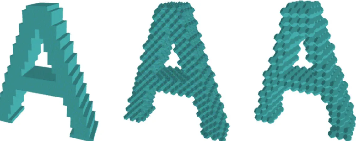
Figure 1.3: A 3D object sampled on the cubic grid (left), the face-centered cubic grid (middle), and the body-centered cubic grid (right).

◦ ◦

◦

◦ • p •

◦

◦ ◦ • ◦ ◦

◦ ◦

• ◦

◦

◦ • p

• ◦

◦ ◦ ◦

◦ • ◦

• p •

◦ • ◦

• •

• p •

• •

Figure 1.4: Adjacency relations on the three possible regular planar grids.

Points that are 1-adjacent to the central pointpare marked ‘•’, while points being 2-adjacent but not 1-adjacent topare marked ‘◦’. (Note that relations on the triangular grid for ‘∆’ and ‘∇’ points are differentiated.)

spectively. Hence, 1-adjacency and 2-adjacency are also called, respectively, 3-adjacency and 12-adjacency [133, 184]. Note that the triangular grid is formed by two kinds of points: ∆-triangles and ∇-triangles (see Figure 1.4).

Without loss of generality, throughout this dissertation the topological properties of the triangular grid are illustrated for ‘∆’ points.

In the conventional square grid,N₁^∗^Z²(p) contains 4 elements, andN₂^∗^Z²(p) is formed by 8 elements. That is why they are often referred to as 4-adjacency and 8-adjacency, respectively [133, 137, 184]. In the case of hexagonal grid, N₁^∗H(p) = N₂^∗H(p) contains 6 elements, hence these two relations are also called 6-adjacency [184].

In the 3D cubic grid Z³ two points are 6-adjacent, 18-adjacent, and 26- adjacent if the associated Voronoi cells (i.e., unit cubes) share a face, share a face or an edge, and share a face, an edge, or a vertex, respectively.

Note that all the three binary relations are reflexive and symmetric. Let us denote the set of points that arej-adjacent to a point p∈Z³ by N_j^Z³(p), and let N_j^∗^Z³(p) =N_j^Z³(p)\ {p}(j = 6,18,26) (see Figure 1.5).

(15)

✑✑

⋆ ⋆ S

⋆ ⋆ U

W p E

D

⋆ ⋆ N

⋆ ⋆

✑✑

Figure 1.5: Frequently used adjacency relations in Z³. The set N₆^Z³(p) contains point p and the six points marked U, D, N, E, S, and W. The set N₁₈^Z³(p) contains N₆^Z³(p) and the twelve points marked ‘’. The set N₂₆^Z³(p) contains N₁₈^Z³(p) and the eight points marked ‘⋆’.

1.1.3 Binary Digital Pictures

Let us consider the adjacency relation j (j = 1,2) on a regular planar grid.

A point p ∈ V is j-adjacent to a set of points X ⊆ V if there is a point q∈X such that q∈N_j^V(p) [137].

A sequence of distinct points hp₀, p₁, . . . , p_miin V is called a j-path from p₀ to p_m in a non-empty set of pointsX ⊆ V if each point of the sequence is inX and p_i is j-adjacent to p_i−1 for each i= 1,2, . . . , m. Note that a single point is a j-path of length 0.

Two points are said to bej-connected in a set X if there is aj-path inX between them. A set of pointsX isj-connected in the set of pointsY ⊇X if any two points in X are j-connected in Y. Aj-component of a set of points X is a maximal (with respect to inclusion) j-connected subset ofX. Figure 1.6 illustrates the components of a set X ⊂Z².

In their seminal work [137], Kong and Rosenfeld defined a binary digital picture as follows:

Definition 1.1.1 [137] A (k,¯k) binary digital picture(or, in short picture) on grid V is a quadruple (V, k,¯k, B), where B ⊆ V is the set of black points (consequently, V \B is the set of white points),k-adjacency and ¯k-adjacency are used for B and V \B (k,k¯∈1,2), respectively.

For practical purposes, we assume that all pictures are finite (i.e. they contain finitely many black points).

Ablack component orobject is ak-component ofB, while awhite compo- nent is a ¯k-component ofV \B. In a finite picture there is a unique infinite

(16)

8 9 7 7

6 7 7

5 4

1 3 4

1 1 2

1 2 2 2 2

Figure 1.6: The set of points X ⊂ Z² depicted in black. There are nine 1- components ofX, where all points labeled by ‘i’ belong to thei-th component (i= 1, . . . ,9). Note that X forms just one 2-component.

white component, which is said to be the background, and a finite white component is called acavity¹.

A black pointpis called aninterior point if all points inN_¯_k^∗V(p) are black.

A black point is said to be aborder point if it is not an interior point (i.e., it is ¯k-adjacent to at least one white point). A (black) border-pointp is called an isolated point if all points in N_k^∗V(p) are white (i.e., {p} is a singleton object).

In order to avoid connectivity paradoxes [137], and verify the discrete Jordan’s theorem [184], different adjacency relations are usually taken into consideration for the black and white points (i.e., k 6= ¯k).

All concepts reviewed in the 2D case can be extended to the cubic grid Z³. In this work, our attention has been focussed on (26,6) pictures.

A black point p in picture (Z³,26,6, B) is called an interior point if N₆^∗^Z³(p) ⊂ B (i.e., all 6-neighbors of p are black). A black point p in this picture is said to be a border point if it is not an interior point (i.e., it is 6- adjacent to at least one white point). A black pointpin picture (Z³,26,6, B) is called ad-border point if its 6-neighbor marked d in Figure 1.5 is a white point (d ∈ {U,D, N, E,S, W }).

1Some researchers use the termholeto refer to finite white components in 2D pictures, and the ‘tunnel’ that a 3D doughnut (torus) has is said to be a hole, as well. To avoid possible confusion, we reserve the termcavity to refer to finite white components in arbitrary

(17)

1.2 Topology-Preserving Operators

Topology preservation is a major concern in topological algorithms. It is crucial to guarantee that an operator preserves the topology for all possible pictures.

This section defines the concepts of an operator and a simple point, and reviews some sufficient conditions for topology preservation.

1.2.1 Operators

Recall that only two possible values are assigned to each grid point in a (binary digital) picture. It is assumed that these two values are black (1) and white (0).

Let T be an operator that transforms the input picture with the set of black points B into the output picture in which the set of black points is denoted by T(B). A local operator gives each point p a ‘new’ value that depends only on the ‘old’ values of the local neighborhood or support of p. If the support contains n points, local operator T is specified by its alteration rule f_T : {0,1}ⁿ→ {0,1} that is a Boolean function of n variables.

OperatorTis called areduction ifT(B)⊆B for each possible set of black pointsB. Hence, reductions transform pictures only by changing some black points to white ones which is referred to as deletion. Operator T is said to be an addition if B ⊆ T(B) for each B. Thus additions change only some white points which is referred to as filling. An operator which does not fall into either of these two categories is called a mixed operator.

Note that reductions play a key role in various topological algorithms, e.g., thinning [89, 147, 324] (i.e., iterative object reduction to extract skeleton- like features) or reductive shrinking [90] (i.e., that is capable of producing a minimal structure that is topologically equivalent to the original object).

Parallel operators can change a set of points simultaneously, while se- quential operators traverse the points of a picture, and focus on the actually visited single point for possible alteration [90]. Evidently, the result of a sequential operator may depend on the visiting order which is applied.

1.2.2 Topology Preservation in Reductions

In [319], Stefanelli and Rosenfeld laid down the following criterion for topology- preserving 2D reductions:

Criterion 1.2.1 [319] A reduction (acting on 2D pictures) preserves the topology if and only if the following conditions all hold:

(18)

1. It never splits an object into two or more.

2. It never deletes completely any object in the input picture.

3. It never merges a cavity in the input picture with the background or another cavity.

4. It never creates a cavity where there was none in the input picture.

Figure 1.7 illustrates a 2D reduction that is not topology-preserving.

b b b

d a e

c

→

b b b

d a e

c

Figure 1.7: A reduction for a (2,1) picture on Z² that is not topology- preserving. Deletion of the point marked ‘a’ splits the larger object into two; the smaller object is completely deleted by deleting the points marked

‘b’; deletion of the point marked ‘c’ merges a cavity with the background;

the remaining two cavities are merged with each other by deleting the point marked ‘d’; deletion of the point marked ‘e’ creates a brand new cavity.

In effect, Criterion 1.2.1 was rephrased as follows:

Criterion 1.2.2 [137] Let(V, k,k, B)¯ be a (2D) picture. The deletion of the set of points D⊂B preserves the topology if and only if

1. each k-component ofB contains exactly onek-component ofB\D, and 2. each k-component of¯ V \(B\D) contains exactly one ¯k-component of

V \B.

Note that Criteria 1.2.1 and 1.2.2 are only valid in 2D.

There is an additional concept called a hole (or a tunnel) in 3D pictures [137, 139]. Holes (of the kind that doughnuts have) are formed by white points, but they are not white components. Topology preservation implies that creating, eliminating, and merging holes are not allowed (see Figure 1.8).

That is why the proposed criteria for topology-preserving 3D reductions are rather complicated [137]. They are based on digital deformation of closed paths and a digital fundamental group introduced by Morgenthaler [193] and Kong [136], respectively.

(19)

→

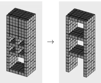
Figure 1.8: A 3D reduction that satisfies all conditions of Criteria 1.2.1, but is not topology-preserving on (26,6) pictures, since a hole not present in the input picture is created, a hole is eliminated, and four holes are merged with each other.

1.2.3 Simple Points

General conditions for topology preservation were obtained with the help of the concept of a simple point [137]. Since we have dealt with all the three kinds of operators (i.e., reductions, additions, and mixed operators), we have respect for the following definition²:

Definition 1.2.1 A black point in an arbitrary picture is a simple point if and only if its deletion preserves the topology (i.e., it is a topology-preserving reduction). Likewise, a white point in an arbitrary picture is a simple point if and only if its filling preserves the topology (i.e., its filling is a topology- preserving addition).

Kardos and Pal´agyi gave unified formal characterizations of simple (black or white) points in the given five types of 2D pictures:

Theorem 1.2.1 [122, 126]Let p be a point in a picture(V, k,¯k, B). Then p is simple if and only if the following conditions hold:

1. p is k-adjacent to exactly one k-component of N₂^∗V(p)∩B. 2. p is ¯k-adjacent to exactly one ¯k-component of N₂^V(p)\B.

2Since the attention of most researchers has been focused only on reductions, it is

(20)

Theorem 1.2.1 shows that simplicity of a point p is a local property: it can be decided by examining the set N₂^∗V(p) containing just 12, 8, and 6 points for T, Z², and H, respectively. As a straightforward consequence of the above theorem we note that if a black point is an isolated or interior point then it is not simple (i.e., some border points may be simple). Another immediate consequence of Theorem 1.2.1 is the following duality theorem:

Theorem 1.2.2 A point pis simple in picture (V, k,¯k, B)if and only if pis simple in picture(V,k, k,¯ V \B)(i.e., in the picture that is obtained from the former by swapping the black and white sets of points and their associated adjacency relations).

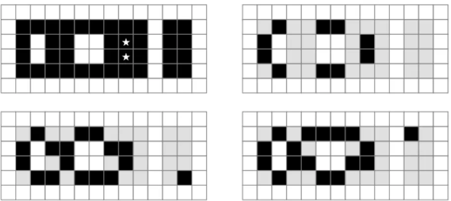
Figure 1.9 gives some examples of simple and non-simple points in (1,2) and (2,1) pictures on Z².

p p p p

(a) (b) (c) (d)

Figure 1.9: Examples of simple and non-simple points in (1,2) and (2,1) pictures on Z². Point p is simple in both (1,2) and (2,1) pictures (a); p is simple in (1,2) pictures and it is non-simple in (2,1) pictures (b); p is non- simple in (1,2) pictures and it is simple in (2,1) pictures (c);pis non-simple in both (1,2) pictures and (2,1) pictures (d). Note that p may be either a black or a white point.

In [139], Kong proposed an easily visualized characterization of simple points on (2,1) pictures on Z² by using the concept of an attachment set. Kardos and Pal´agyi adapted Kong’s model for all the three regular planar grids [120, 124].

We should add that Kardos and Pal´agyi illustrated simple points in all the given five types of 2D pictures by a few configurations (so-called matching templates), which make an efficient implementation of the verification of simplicity possible [122, 124, 126].

Malandain and Bertrand established the following characterization of simple points on the 3D (26,6) pictures on Z³:

Theorem 1.2.3 [179] Let p be a point in a picture (Z³,26,6, B). Then p is simple in that picture if and only if all the following conditions hold:

(21)

1. N₂₆^∗^Z³(p)∩B contains exactly one 26-component.

2. N₆^∗^Z³(p)∩(Z³\B)6=∅(i.e.,p is6-adjacent to at least one white point).

3. Any two points inN₆^∗^Z³(p)∩(Z³\B)is6-connected in the setN₁₈^∗^Z³(p)∩ (Z³\B).

Similarly to the examined 2D cases (see Theorem 1.2.1), the simplicity of a pointpin (26,6) pictures is a local property: it can be decided by examining the set N₂₆^∗^Z³(p). Figure 1.10 gives some examples of simple and non-simple points in (26,6) pictures on Z³.

✑✑

✑✑ (a)

• • ◦

◦ ◦ ◦

◦

^p

◦

◦ ◦ ◦

◦ • •

✑✑

✑✑ (b)

◦ ◦ ◦

◦ • ◦

◦ ◦ ◦

◦ • ◦

•

^p

• ◦ • ◦

◦ ◦ ◦

◦ • ◦

◦ ◦ ◦

✑✑

✑✑ (c)

◦ ◦ ◦

◦ • ◦

◦ ◦ ◦

•

^p

• ◦ ◦ ◦

◦ ◦ ◦

◦ • ◦

◦ ◦ ◦

✑✑

✑✑ (d)

◦ ◦ ◦

◦ • ◦

◦

^p

◦

• ◦ •

◦ ◦ ◦

◦ ◦ •

◦ ◦ ◦

✑✑

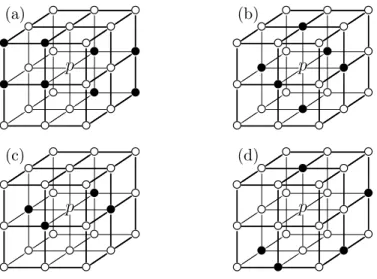
Figure 1.10: Examples of simple and non-simple points in (26,6) pictures on Z³. In configuration (a), p is not simple (since Condition 1 of Theorem 1.2.3 is violated); in configuration (b), p is not simple (since Condition 2 of Theorem 1.2.3 is violated); in configuration (c), p is not simple (since Condition 3 of Theorem 1.2.3 is violated); in configuration (d), p is simple since all the three conditions of Theorem 1.2.3 are satisfied.

Note that Kong extended his characterization of simple points in (2,1) pictures on Z² by using attachment sets to 3D (26,6) pictures [139].

1.2.4 Sufficient Conditions

Let us see first three general sufficient conditions for topology preservation (i.e., conditions that are valid for arbitrary binary pictures).

Altering a single pointpin a picture preserves the topology if and only ifp is simple in that picture (see Subsection 1.2.3). Parallel operators can change

(22)

a set of points at a time. Hence, we need a precise definition of what is meant by topology preservation when a number of points are changed (deleted or filled) simultaneously.

Definition 1.2.2 [139, 168]Let P be an arbitrary picture. A set ofn points Q is a simple set³ in P if it is possible to arrange the elements of Q in a sequence hq₁, . . . , q_ni such that q₁ is a simple point in P and each q_i is simple after the set of points {q₁, . . . , q_i−1} is changed (i= 2, . . . , n). Such a sequence is called asimple sequence. (And let the empty set be called simple.)

Figure 1.11 gives examples of simple and non-simple sets of black points in a (2,1) picture on the grid Z².

h i j e f g c d a b

Figure 1.11: Examples of simple and non-simple sets in picture (Z²,2,1,{a, . . . , j}). The set of black points {a, b, c, d} is simple since all the 12 sequences (of the possible 24 ones) ha, b, c, di, ha, b, d, ci, ha, c, b, di, ha, d, b, ci, hb, a, c, di, hb, a, d, ci, hb, c, a, di, hb, d, a, ci, hc, a, b, di, hc, b, a, di, hd, a, b, ci, and hd, b, a, ci are simple. The set of black points {f, i} is non- simple, since both sequenceshf, iiandhi, fiare non-simple. (Note that each black point is simple. Hence, all the 10 singleton sets{a}, . . . ,{j}are simple sets.)

There is general agreement that the concept of a simple set trivially implies a sufficient condition for topology-preserving parallel operators:

Criterion 1.2.3 [139, 168, 272] A parallel operator is topology-preserving if, for all possible pictures, it changes only simple sets.

Bertrand [23] and Kong [139] reported alternative solutions to the prob- lem: they introduced the notions of a P-simple set and a hereditarily sim- ple set, respectively, whose simultaneous deletion is proved to be topology- preserving.

3Since most researchers have studied only reductions, it is usually assumed that a simple set is a subset of black points. We have dealt with all the three kinds of operators (i.e., reductions, additions, and mixed operators), hence there may be white points in ‘our’

(23)

Definition 1.2.3 [23] Let P= (V, k,¯k, B) be an arbitrary picture. A set of black pointsQ⊂B is a P-simple set in Pif for any point q ∈Q and any set of points R ⊆Q\ {q}, q is simple in picture (V, k,¯k, B\R). Each element of a P-simple set is called a P-simple point.

Theorem 1.2.4 [23] A reduction that deletes a subset composed solely of P-simple points is topology-preserving.

Note that Bertrand gave a local characterization of P-simple points in (26,6) pictures on Z³ [23]. Later Bertrand and Couprie proposed a similar characterization in (2,1) pictures on Z² [27], and Kardos and Pal´agyi presented both formal and easily visualized sufficient and necessary conditions of P-simple points in all the given five types of 2D pictures [125].

Figure 1.12 shows a P-simple set in a (2,1) picture on Z².

⋆ ⋆

⋆

⋆ ⋆ ⋆

⋆ ⋆

⋆ ⋆ ⋆

⋆ ⋆

⋆ ⋆ ⋆

⋆ ⋆

⋆ ⋆ ⋆

⋆ ⋆ ⋆ ⋆ ⋆

Figure 1.12: Example for a P-simple set in a (2,1) picture onZ². Non-simple black points are depicted in black, simple black points are depicted in gray, elements in a P-simple set are marked ‘^⋆’. Note that all possible P-simple sets are subsets of simple points.

Definition 1.2.4 [139] A set of black points Q is said to be hereditarily simple in a picture if all subsets of Q (including Q itself ) are simple sets in that picture.

Theorem 1.2.5 [139] A reduction that deletes only hereditarily simple sets is topology-preserving.

To ensure topology preservation for parallel reductions, Ronse gave the following specific sufficient condition:

(24)

Theorem 1.2.6 [272] A parallel reduction R acting on (2,1)pictures on Z² is topology-preserving, if all the following conditions hold:

1. Only simple points are deleted by R.

2. For any two1-adjacent black pointspandq that are deleted byR,{p, q} is a simple set.

3. R never deletes completely any object contained in a 2×2 square (i.e., a set of four mutually 2-adjacent points).

Ma [168] and Kong [139] gave the foremost sufficient condition for topology- preserving reductions on 3D (26,6) pictures. They introduced the concepts of a unit lattice square and a unit lattice cube: a unit lattice square in Z³ is formed by four mutually 18-adjacent points, and a unit lattice cube is a set of eight mutually 26-adjacent points (see Figure 1.13).

✑✑ ✑✑

✑✑

✑✑ ✑✑

⋆ ⋆

⋆ ⋆ ^✑^✑ ^✑^✑

⋆ ⋆

⋆ ⋆ ^✑^✑

✑✑

⋆

(a) (b) (c) (d)

Figure 1.13: A unit lattice cube (a), and three unit lattice squares (b)-(d).

Their corners (i.e., points in Z³) are marked ‘⋆’. (Notice that each ‘face’ of a unit lattice cube is a unit lattice square.)

Theorem 1.2.7 [139, 168] A 3D parallel reduction R acting on (26,6) pic- tures is topology-preserving if all the following conditions hold:

2. For any two black points pand q contained in a unit lattice square that are deleted by R, {p, q} is a simple set.

3. For any three black points p, q, and r contained in a unit lattice square that are deleted by R, {p, q, r} is a simple set.

4. For any four black points p, q, r, and s contained in a unit lattice square that are deleted by R, {p, q, r, s} is a simple set.

5. R never deletes completely any object contained in a unit lattice cube.

(25)

In order to verify the topological correctness of some 3D thinning algorithms, Pal´agyi and Kuba [221] proposed a simplified condition⁴:

Theorem 1.2.8 [221] A 3D parallel reduction R acting on (26,6) pictures on Z³ is topology-preserving if all the following conditions hold:

2. Let p∈B be any point in a picture (Z³,26,6, B) such that p is deleted by R. Let Q⊂ B\ {p} be any set of points that are deleted by R from picture (Z³,26,6, B) such that Q∪ {p} is contained in a unit lattice square. Then p is simple in picture (Z³,26,6, B\Q).

3. R never deletes completely any object contained in a unit lattice cube.

4This result originated before defending the author’s Ph.D. dissertation in the year

(26)

1.3 Skeletonization

In his seminal work [32], Blum introduced a shape feature called skeleton that jointly describes the topology and the geometry of a binary object. The skeleton of a continuous object in Rⁿ was historically given by the Medial Axis Transform (also-called Symmetry Axis Transform), which tracks the points having at least two closest boundary points. It can be defined in two alternative ways:

• Blum’s grassfire (or prairie-fire) propagation assumes that the object is a field of dry grass and its entire boundary is set on fire at a time. It is also supposed that the fire spreads in all directions with equal velocity.

Then the skeleton is the set of points where the concurrent fire fronts meet and quench each other (see Figure 1.14).

• The skeleton is the loci of the centers of all maximal inscribed hyperspheres (i.e., disks in 2D, balls in 3D, etc.), where a hypersphere is inscribed if it is completely included by the object, and it is maximal if it is not covered by any other inscribed hypersphere (see Figure 1.15).

The equivalence of the above two approaches was proved by Calabi and Hartnett [46, 92].

Figure 1.14: Illustrating the prairie-fire propagation for a horse. Colored lay- ers removed by the isotropic object reduction process (left) and the skeleton (right).

The skeleton is a widely used shape descriptor due to its advantageous properties:

• It represents local object symmetries [39, 59, 79, 290].

• It reflects the topological structure of the object to be characterized [45, 188].

(27)

Figure 1.15: Skeleton of a solid (2D) rectangle. Both points ‘A’ and ‘B’

belong to the skeleton, since they have more than one closest boundary points and they are centers of maximal inscribed disks. On the contrary, point ‘C’

is not skeletal, since the corresponding disk is not maximal (i.e., it touches the boundary in just one point).

• It can be used to object decomposition (i.e., to partition an object into a set of primitives) [33, 34, 199].

• It reduces the dimensionality since a 2D object is reduced to 1D curves;

the skeleton of a 3D object may contain just 2D and 1D structures (surfaces and curves) [59, 79, 199, 280] (see Figure 1.16).

• It is ‘thin’ (i.e., the skeleton contains 1-point width manifolds and offers dramatically less information than the original object) [59, 79].

Figure 1.16: A solid 3D box (left) and its skeleton (right) that contains some 2D surface patches.

The above-defined skeleton assumes continuous approach. Since we deal with digital pictures, skeletonization means extraction of skeleton-like fea- tures from digital binary objects [42, 54, 280]. These features are presented in Subsection 1.3.1.

Subsection 1.3.2 describes the major skeletonization approaches, and applications are reviewed in Subsection 1.3.3.

(28)

1.3.1 Skeleton-Like Features in 2D and 3D

In 2D, two kinds of skeleton-like features are taken into consideration (see Figure 1.17): the centerline that approximates the continuous skeleton, and the topological kernel that is a minimal set of points being topologically equivalent [137] to the original object (i.e., if we remove any further point from it, then the topology is not preserved). If an object does not contain any cavity, its topological kernel is an isolated point. Otherwise, topological kernels are formed by 1-point thick closed curves.

Figure 1.17: Centerline (left) and topological kernel (right) superimposed on a 2D (discrete) object.

In the 3D case, there are three types of skeleton-like features: the cen- terline, the medial surface (see Figure 1.18), and the topological kernel (see Figure 1.19).

The centerline in 3D is a line-like or stick-like 1D representation of objects that captures the part-whole structure of the object to be described [53, 307].

In many applications (see Subsection 1.3.3), it is a concise representation of tubular and tree-like 3D objects. The medial surface provides an approxi- mation to the the continuous 3D skeleton, since it can contain 2D surface patches. Similarly to the 2D topological kernel, a topological kernel of a 3D object is a minimal set of points that is topologically equivalent to the original object. It is fairly useful in representing or checking the topological structure of the object to be described. Note that a topological kernel of a 3D object is an isolated point if and only if it does not contain any holes nor

Figure 1.18: Centerline (left) and medial surface (right) superimposed on a 3D image of a biplane.

(29)

cavities.

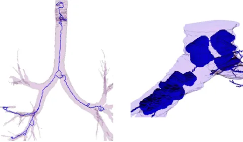
Figure 1.19: Topological kernels superimposed on incorrectly segmented 3D human airway trees. Since the segmented trees contain some holes (left) and some cavities (right), there are some closed ‘thin’ curves (loops) and some

‘bubbles’ (cavities) with one point thick walls in their topological kernels.

It is an important property of (2D and 3D) centerlines that they contain just three types of elements: endpoints (which have only one skeletal neighbor), line-points (that are ‘adjacent’ to exactly two skeletal points), and branch-points (that have more than two skeletal neighbors) that form junc- tions (bifurcations, trifurcations, etc.). Hence, a complex descriptor named skeletal graph⁵ can be derived from centerlines. The set of vertices of a skeletal graph is formed by the endpoints and the branch-points, and there is an edge between two vertices if they are connected via ‘adjacent’ line-points [15, 16, 41, 62, 109, 167, 177, 231, 269, 273] (see Figures 1.20 and 1.21).

Lastly, we mention that Pizer et al. [256, 258] proposed a particular type of shape feature calleddeformable m-reps (a sampled medial object representation). It is derived from the medial surface of a 3D object, and represents 3D object boundaries using sheets of medial atoms [304].

1.3.2 Skeletonization Techniques

Several approaches have been proposed for producing skeleton-like features from (segmented) binary objects. Some authors presented comprehensive

5Some researchers use the termskeleton graph for the same shape descriptor. That is ambiguous, since the notion of skeleton graph also means a particular edge- and vertex-

(30)

Figure 1.20: A 3D centerline with the three types of elements (left), the derived skeletal graph (right).

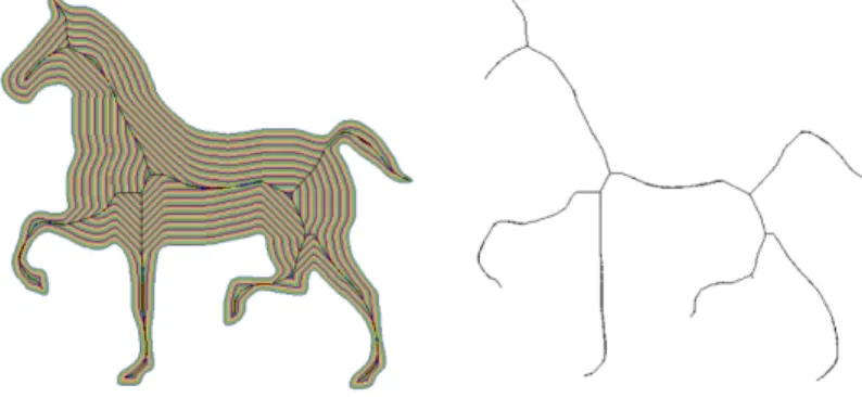
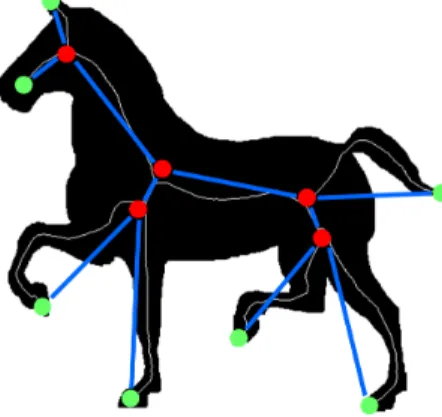
Figure 1.21: Centerline superimposed on a 2D image of a horse and the corresponding skeletal graph.

and concise surveys [278, 279, 280, 282, 304, 307, 330]. Here we summarize the three major skeletonization techniques: generation from distance maps, geometric approach based on Voronoi diagrams, and modeling the fire-front propagation (thinning).

Distance-based skeletonization refers to the definition of the (continuous) skeleton by the centers of all maximal inscribed hyperspheres. It usesdistance maps that are the results of distance transform algorithms [35]. The input of a (discrete) distance transform algorithm is a binary picture in which white points form the set of feature points, and it is converted into a (non binary) array, where each element has a value that gives the distance to the

‘nearest’ feature point. The produced distance map strongly depends on the applied distance [86]. The most popular ones are distance family derived from adjacency relations [35, 321], weighted or chamfer distances [35, 322],

(31)

quasi-Euclidean distances [35, 60, 191], and the exact (error-free) Euclidean distance [67, 189, 284, 353]. Note that computing distance transform takes linear time in arbitrary dimensions [35, 189].

If a distance transform is calculated from the white points in a binary picture, some local maxima in the distance map form centerlines in 2D, and medial surfaces in the 3D case. These ‘ridges’ have been identified by standard techniques of differential geometry and heuristic methods [5, 36, 270].

Note that distance-based skeletonization can produce geometrically accu- rate features (from exact Euclidean distance maps), but some ridge-detectors cannot provide topologically correct results.

The Voronoi skeleton is obtained by computing the Voronoi diagram of sampled boundary points [3, 280, 329]. In [289], Schmitt has shown that if the density of the sampled boundary points uniformly goes to infinity, the ‘internal’ elements of the corresponding Voronoi diagram converges to the (exact continuous) skeleton. Several authors proposed computationally efficient algorithms for computing the Voronoi diagram [40, 131, 202, 216, 262]. The raw Voronoi skeleton may contain a large number of spurious branches in 2D, and unwanted surface patches in the 3D case. Thus the Voronoi skeletonization is to be paired with a proper pruning method [12, 202, 217, 218].

Although the Voronoi skeleton is correct in both geometrical and topological senses, this method is rather time-consuming and ‘hybrid’ (i.e., its input is a discrete set of points, but the output if formed by continuous segments).

The third major skeletonization technique is the digital simulation of the fire-front propagation. Thinning [89, 147, 280, 307, 324] is an iterative object-reduction process for producing any skeleton-like feature in a topology-preserving way: the outmost layer of an object is deleted, and the entire process is repeated until stability is reached (see Figure 1.22).

Most of the existing thinning algorithms are parallel, since the fire-front propagation is parallel by nature [8, 22, 25, 27, 28, 29, 56, 57, 58, 82, 88, 89, 113, 115, 120, 121, 147, 150, 162, 165, 166, 168, 169, 170, 171, 172, 174, 175, 180, 181, 203, 204, 205, 206, 208, 209, 210, 211, 219, 220, 221, 222, 225, 229, 232, 233, 234, 235, 236, 237, 242, 243, 244, 246, 248, 268, 275, 276, 324, 338, 354, 358]. We should add that some sequential algorithms have also been proposed [55, 112, 114, 116, 117, 147, 150, 197, 198, 224, 240, 242, 243, 244, 246, 252, 266, 320, 324].

The topology-oriented thinning pays less attention to the metric properties of the object to be represented, since the invariance under arbitrary rota- tion angles or scaling factors is not fulfilled. In spite of these drawbacks, our attention has been focussed on thinning, since thinning is the fastest skeletonization method, it can be implemented easily, it can produce all types of

(32)

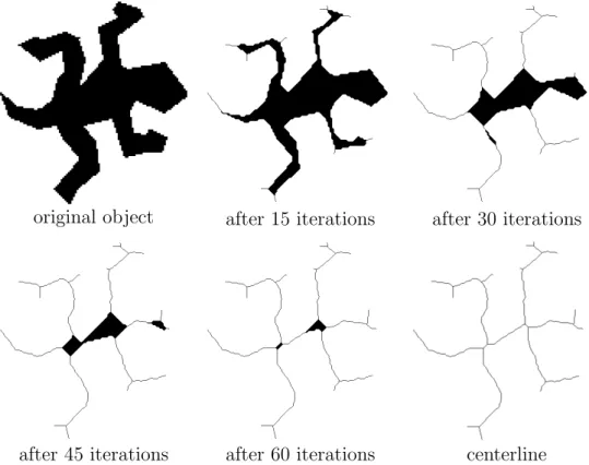
original object after 15 iterations after 30 iterations

after 45 iterations after 60 iterations centerline

Figure 1.22: Thinning of Escher’s (rep)tile. Some phases of the iterative object reduction are shown.

skeleton-like features, the topology-preservation is guaranteed, and thinning provides practically exquisite descriptors for a number of applications.

Note that there are some additional skeletonization approaches:

• Some attempts have been made to approximate the result of Medial Axis Transform in discrete spaces. The ‘skeletons’ are defined in terms of a new concept, called the Integer Medial Axis (IMA) transform [98, 186].

• Distance transform has been combined with thinning. Some authors proposed skeletonization algorithms in which the distance transform is followed by (non-iterative) sequential deletion of ‘deletable’ points in ascending distance order [263, 285, 309]. In [327], ‘peak’ points are detected in distance maps, then these points are preserved by an iterative reductive shrinking.

• The ‘skeleton’ can be expressed in terms of the basic morphological operations [69, 83, 296, 308], where hyperspheres are approximated

(33)

by successive dilations, and the original object can be exactly recon- structed from the the skeletal subsets [149]. Note that some simple thinning algorithms can be described by the morphological hit-or-miss transform (as a basic tool for detecting the ‘deletable’ points of the applied reduction) [83, 133, 184, 296, 308].

• Some authors have used minimal cost method for generating 2D and 3D centerlines (i.e., path optimization can be carried out with graph algorithms) [107, 108, 161].

• Several techniques use continuous curve propagation for simulating the fire-front propagation: active contour [152], anisotropic partial differential equation [365], Gaussian affinity voting [371], principal curves [154], shock of boundary evolution [128, 302], normal field [104, 176], level set [129, 332, 351], flux [37, 255, 303], Markov framework (MRF) [2], absolute scale [11], potential field [1, 51], and gradient vector flow [93].

• Some authors have reported skeletonization algorithms acting on grey- scale pictures and fuzzy objects [6, 7, 31, 106, 173, 183, 266, 283, 293, 297, 331, 363].

Numerous authors have proposed methods to evaluate the performance of skeletonization algorithms [9, 53, 85, 103, 145, 276, 286, 288, 306, 307, 330].

Due to the lack of definition of the ‘true skeleton’ for a discrete object, a widely accepted approach evaluating the goodness of skeletonization algorithms is yet absent [280]. That is why we have proposed a method for the quantitative comparison of ‘skeleton’ features [212]. The two key components of our approach are a specific similarity measure for ‘skeletons’ and a gold standard image database containing pairs of reference objects and their expected results.

1.3.3 Applications of Skeletonization

Skeleton-like features have been widely used in different image processing and computer vision applications. Here, we provide a list of these applications with no claim to completeness: animation [54, 61, 74, 347], chordal surface generation [146], computer graphics [53], coding [100, 158, 143, 182], design and engineering applications [264], fingerprint analysis [68, 84, 369], generating mesh sizing functions [265], measuring shape similarity [336], motion analysis [73, 74], multiscale shape analysis [335], object recognition and classification [11, 16, 62, 95, 291, 300, 362], off-line character recognition

(34)

[10, 65, 148], part-patch segmentation and object decomposition [135, 295], porous filter permeability, analysis of porous media, and pore space morphol- ogy [155, 156, 159, 261, 305, 368], raster-to-vector conversion [18, 253, 310], registration [345], segmentation [44, 53, 257, 259], shape deformation and morphing [30, 361], shape matching and retrieval [15, 41, 49, 53, 54, 70, 80, 96, 104, 167, 178, 213, 267, 325], shape modeling [71, 304, 347], terrain modeling [333], tracing and virtual navigation [53, 101, 104].

Skeletonization has been frequently applied in many medical image processing applications, including airway analysis and virtual bronchoscopy [19, 76, 107, 195, 196, 360, 363], brain tissue analysis [132], characterization of complex anatomic object [38, 202, 367], colonography and virtual colonoscopy [63, 111, 274, 102, 318, 348], estimating the motion of arteries [334], malig- nant tumor identification [134], medical image segmentation and registration [47, 254, 260, 364], mesh generation of tubular geometries [185], neuron traces [344], path planning [352], stenosis detection [50, 72, 85, 215, 288, 351], surgical planning [292], trabecular bone analysis [105, 277, 281, 283], vascular and endovascular surgery, vessel lumen segmentation, angiography, angiogen- esis, and detection of aortic aneurism [4, 48, 78, 91, 151, 154, 157, 261, 194, 214, 271, 301, 337, 349, 350, 355, 356, 359, 366, 370, 371], virtual endoscopy [94, 161], and visualization of tomographic molecular imaging [17].

In [153], Leymarie and Kimia covered a wide spectrum of applications of medical symmetries (including applications in geography, cartography, wire- less sensor networks, urbanism, architecture, archaeology, visual arts, motion analysis, body animation, robotics, machining, industrial design, registration, medicine, and biology).

The author’s 3D thinning algorithms have been involved in the following biomedical applications: assessment of infrarenal aortic aneurysm [224], assessment of tracheal stenosis [224, 311, 313, 315, 316], unraveling and virtual dissection of the colon [224, 312, 314, 317], colorectal polyp detection [314], characterization of the interstitial lung diseases [99], matching and anatomical labeling of human airway tree [339, 341], quantitative analysis of pulmonary airway trees [226, 227, 228, 231], liver segmentation for surgical resection planning [20], and identifying synaptic connections [187].

For reasons of scope, in this dissertation, our method for quantitative analysis of pulmonary airway trees (see Chapter 4) is only described.

(35)

Chapter 2 Topology Preservation

This chapter is to summarize our theoretical results concerning diversified topological problems. These results provide methods of verifying that an operator preserves the topology, allow us to generate topology-preserving operators, and provide computationally efficient thinning algorithms.

For reasons of scope, in this chapter, only some selected results are presented.

Configuration-based and point-based sufficient conditions for topology- preserving reductions are presented for 2D pictures in Section 2.1.

In Section 2.2, both symmetric and asymmetric point-based conditions are given for topology-preserving reductions acting on 3D (26,6) pictures on Z³.

Instead of investigating the sets of altered points, the author proposed a novel sufficient condition for topology-preserving operators that takes the alteration rules of operators into consideration. In Section 2.3, it is described that the general-simple alteration rules provide pairs of equivalent and topology-preserving sequential and parallel operators.

In Section 2.4, the relationships among the five types of sufficient conditions for topology-preserving reductions are reviewed.

(36)

2.1 Sufficient Conditions for 2D Pictures

In this section sufficient conditions for topology-preserving reductions. These results are valid for all the given five types of 2D pictures. Configuration- based conditions provide methods of verifying that an operator preserves the topology, and point-based conditions allow us to generate directly topology- preserving operators.

For reasons of scope, our sufficient conditions for topology-preserving additions [119, 122, 126] and mixed operators [123, 126] are not presented here.

2.1.1 Configuration-Based Conditions for Reductions

In [272], Ronse gave a sufficient condition for topology-preserving reductions in (2,1) pictures on Z² (see Theorem 1.2.6).

Condition 2 of Theorem 1.2.6 examines the simplicity of a set of two points. Thanks to the following (absolutely general and dimensionless) lemma stated by Kardos and Pal´agyi, it can be simplified:

Lemma 2.1.1 [122, 124] Let p and q be two (black) simple points in an arbitrary picture. If premains simple after the deletion of q, then q remains simple after the deletion of p.

Lemma 2.1.1 can be rephrased as follows:

• If a simple set is formed by two simple points, then both possible sequences of its elements are simple sequences.

• If two black points p and q are simple in a picture, then the following two statements are equivalent:

– pis simple after the deletion ofq (i.e.,hq, piis a simple sequence).

– q is simple after the deletion ofp(i.e.,hp, qiis a simple sequence).

In other words, the simplicity of a set of two simple points can be decided by testing just one sequence/permutation of its elements. Hence, no

‘repechage’ is needed.

Condition 3 of Theorem 1.2.6 examines objects contained in a 2×2 square.

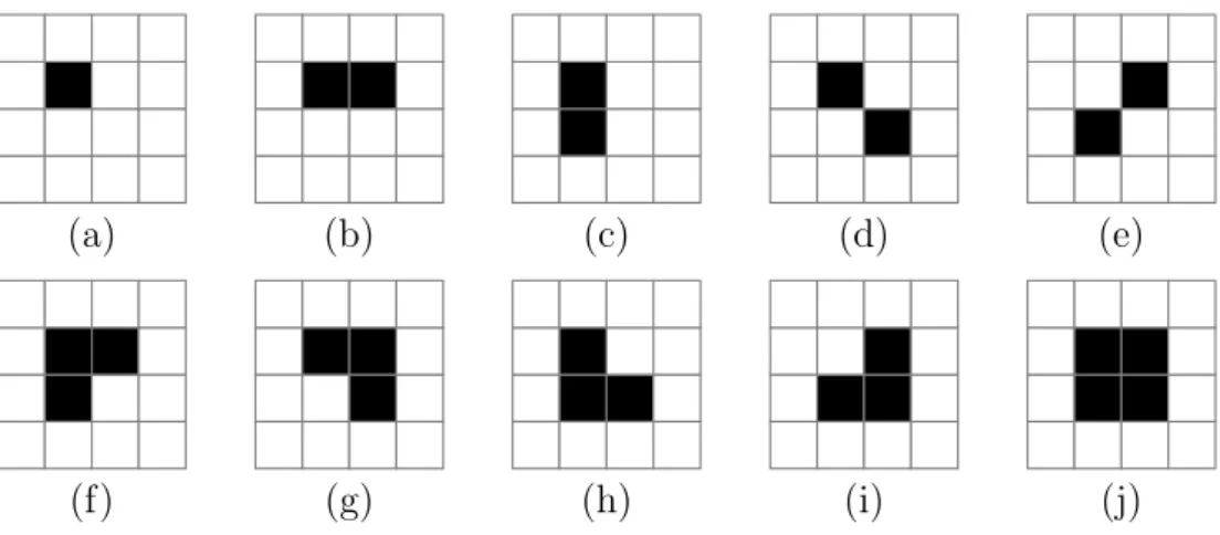
It is easy to check that there are exactly ten such objects (see Figure 2.1).

With the help of Lemma 2.1.1 and Figure 2.1, Ronse’s condition (i.e., Theorem 1.2.6) can be rephrased as follows:

Theorem 2.1.1 [122, 124, 208] A parallel reduction R acting on (2,1) pic- tures on Z² is topology-preserving, if all the following conditions hold:

(37)

(a) (b) (c) (d) (e)

(f) (g) (h) (i) (j)

Figure 2.1: The ten possible objects contained in a 2×2 square.

2. For any two 1-adjacent black points p and q that are deleted by R, p is simple after the deletion of q.

3. R never deletes completely any objects shown in Figure 2.1(d) – Figure 2.1(j).

Note that the object in Figure 2.1(a) is not deleted by Condition 1 of Theorem 2.1.1, and the next two objects shown in Figure 2.1(b) and Figure 2.1(c) cannot be deleted by Condition 2 of Theorem 2.1.1, therefore, Condi- tion 3 of Theorem 2.1.1 is satisfied if the remaining seven objects shown in Figure 2.1(d) – Figure 2.1(j) are not deleted completely.

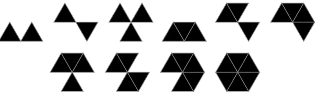
Kardos and Pal´agyi extended Theorem 2.1.1 to all the given five types of 2D pictures [122, 126]. They introduced two notions: the maximal set composed of mutually 2-adjacent points on V is called a unit element (V = T,Z²,H) (see Figure 2.2). An object in a (2,1) picture onV is said to be a small object if it is contained in a unit element, it is not singleton, and it is not formed by two 1-adjacent points (see Figures 2.3-2.5).

Figure 2.2: All the possible unit elements on grids T, Z², and H.

(38)

Figure 2.3: Base small objects in (2,1) pictures on T. All their rotated and reflected versions give all the possible 50 cases.

Figure 2.4: Base small objects in (2,1) pictures grid Z². All their rotated and reflected versions give all the possible 7 cases. (They correspond to the seven objects shown in Figure 2.1(d) – Figure 2.1(j).)

Figure 2.5: The two possible small objects in (1,2) = (2,1) pictures on H.

Theorem 2.1.2 [122, 126] A parallel reduction R acting on (k,k)¯ pictures on V is topology-preserving, if all the following conditions hold:

2. For any two k-adjacent black points¯ p and q that are deleted by R, p is simple after the deletion of q.

3. For the (k,¯k) = (2,1)case, no small object is deleted completely by R.

2.1.2 Point-Based Conditions for Reductions

Condition 2 of Theorem 2.1.2 takes pairs of ¯k-adjacent deleted points into consideration, and Condition 3 deals with small objects. Hence, that theorem states a configuration-based condition, and just provides a method of

Topology Preservation and Thinning