WAVE MECHANICS

CHAPTER SIXTEEN

WAVE MECHANICS

16-1 Introduction

The chapter on wave mechanics is probably subject to more variation in style and content than any other in a textbook of physical chemistry. Wave mechanics is of central importance to the physical chemist: Many of its results are of great utility, as in statistical thermodynamics, chemical bonding, and molecular spectro- scopy. It is also the most nearly correct theory of mechanics that we have and its very language has permeated chemistry. On the other hand, it is difficult to present.

Wave mechanics is virtually unique in the history of scientific theories in that it introduces a mathematical rather than a physical model of nature—and its mathematics becomes so fiercely complicated for systems of chemical interest that its practice has developed into the very specialized field of discovering and evaluating various approximation methods.

It is true, however, that the wave equation can be solved exactly for certain simple or model cases: A particle confined to a box or potential well, the hydrogen atom, and the harmonic oscillator are important illustrations. Most of the approxi- mation methods use combinations or modifications of the exact solutions for such cases, and the procedure in this chapter will be to describe some of these exact solutions in sufficient detail that the rationale of the more advanced approaches can be appreciated. Moreover, most of the language and qualitative thinking in wave mechanics draws on the results for the simple situations. This will be true in Chapter 17 on chemical bonding and again in Chapter 19, on molecular spectroscopy.

The detailed treatment of the important model situations is thus both highly utilitarian and within the spirit of a course in physical chemistry. It might be thought, from all this, that the older quantum chemistry, as exemplified by the Bohr model, would be useless. However, the Bohr theory does give rough descriptions of the quantum states of an atom and also provides some of the terminology of modern spectroscopy. Spectroscopy, as part of the physical chemistry of electronic excited states, is taken up in Chapter 19. For the moment,

we shall content ourselves with a brief review of Bohr's picture for the hydrogen 655

atom. Also, although the origins of quantum theory lie in the development of the quantum treatment of blackbody radiation by Max Planck (around 1900), that subject itself is not ordinarily of great utility to the physical chemist and its outline is placed in a Special Topics section. It is of importance, however, to note here that Planck proposed and successfully defended the hypothesis that molecular oscillators can only have frequencies that are integral multiples of a fundamental, and that the energy of the oscillator is given by

€ = hv, 2hv, 3 h v , ( 1 6 - 1 ) where ν is the fundamental frequency and Λ is a proportionality constant, now called Planck's constant. In the cgs system, h = 6.6256 χ 1 0 "^{2 7} erg sec. Planck's ideas marked the beginning of quantum theory.

Einstein added a vital complement to Planck's hypothesis in explaining how it was that in the photoelectric effect the energy of electrons ejected from a metal by incident light had a definite energy which was independent of the energy flux of the light. Einstein (1905) proposed that light comes in units of energy, or quanta, of value given by the following equation, with ν now the frequency of the light radiation:

e = hv. (16-2) Each quantum ejects one electron and since the energy of the quantum is definite,

so also is the energy of the electron. Increasing the flux of incident light merely increases the number of photoelectrons, their energy being determined by the wavelength or the frequency of the radiation. Wavelength and frequency are related, of course, by the equation

λν = c, (16-3) where λ is the wavelength and c the velocity of light (3.00 χ 10^{1 0} cm s e c^{- 1} in

vacuum). Later, in the period 1908-1912, Einstein extended his law to photo­

chemistry, saying that the absorption of each quantum of light results in the activation or excitation of a molecule by an energy corresponding to that of the quantum. This law of photochemical equivalence is honored by the unit called the einstein', an einstein is one mole of light quanta.

Equation (16-2) is sometimes called the Planck-Einstein equation, in reflection of its general implications. An oscillation of frequency v, associated with atomic oscillators, electrons, or electromagnetic radiation, has energy hv. Absorption of a quantum of light changes the energy of an atom or molecule by hv, and, con­

versely, if an atom or molecule changes energy by an amount and thereby radiates light, that light will be of frequency given by

J e = hv. (16-4) The origins of wave mechanics trace back to Einstein's special theory of rela­

tivity, which led him to conclude that mass m and energy e are interconvertible,

β = mc². (16-5)

One of the important implications of Eq. (16-5) was perceived by L. de Broglie in 1923 as he puzzled over the fact that electromagnetic radiation sometimes appears to behave as particles or quanta, as, for example, illustrated by the law of photo­

chemical equivalence, and yet also appears to behave as waves, as in diffraction

16-1 INTRODUCTION 657 effects. Equation (16-5) provided a connection between these two aspects; if a light quantum has energy Λν, then it must have mass, given by mc² = hv, and momentum p,

hv h ^ ρ = mc = — = - . (16-6)

The intuitional leap made by de Brogue was to see that if radiation could have this duality, so might particles as well. Equation (16-6) provided the connecting link. Although light must always have velocity c (in vacuum, at least), a particle may have some arbitrary velocity v. The generalization of Eq. (16-6) to both radiation and particles is

P = \ , (16-7)

where, for a particle, ρ = mv. Dramatic verifications of de Brogue's equation (16-7) followed. It was found, for example, that electrons show diffraction effects and therefore a wave nature, and today, even neutrons are used in the study of crystal structures by diffraction, their wavelengths being determined by their velocities through Eq. (16-7). Many qualitative features of the wave mechanical theory that followed are derivable just from de Broglie's equation.

The remaining principle that completes the foundations of wave mechanics was formulated by Heisenberg (1927). It is called the uncertainty principle or, sometimes, the principle of indeterminacy. The principle states that neither the position nor the momentum of a particle (or of a light quantum) can be determined with unlimited accuracy, and that if the two quantities are determined simul­

taneously, the minimum uncertainty in each is such that

ΔρΔχ^±.

(16-8)

Equation (16-8) refers to the ultimate obtainable accuracy; any actual experiments will, of course, probably be far less accurate. We consider here only the currently conventional interpretation. See Commentary and Notes, however, for more discussion; there is an important alternative viewpoint as to what is meant by the uncertainty principle.

The uncertainty principle may be stated in alternative ways, since there are other pairs of quantities which determine the state of a particle and whose product has the dimensions of h. The product of the minimum uncertainty in each will then be equal to Α/4π. F o r example, a very useful alternative form states that

(16-9) where At is the uncertainty in the time at which a measurement of energy is made.

Equation (16-9) can be applied to a fluorescing excited state (see Section 19-4).

Quite apart from instrument error, there is always some finite range of frequencies or linewidth for the fluorescent emission of light, which makes the energy of the emitting excited state somewhat uncertain. The rate constant for fluorescent emission gives the average lifetime of the state [see Eq. (14-13)] and this lifetime is a measure of the uncertainty as to just how long a particular excited molecule has lived before emitting. The product of these two uncertainties is h.

The Planck-Einstein, de Broglie, and Heisenberg principles largely demolished

where ν is the reciprocal of the wavelength of the emitted light corresponding to a particular line and is called the wavenumber and n^x and n² are integers. The Balmer series is accurately given by n² = 2 and n^± = 3, 4, 5,... ; the Lyman series, by n² = 1 and n^x = 2, 3, 4,... ; and the Paschen series by n² = 3 and η^λ = 4, 5, 6 , . . . . The same constant 0t applies to all the series, and is called the Rydberg constant.

The modern value for @ is 109,677.581 c m -¹.

Bohr had available in 1913 this very precise, very regular, and as yet mysterious spectral data, although by 1912 J. Nicholson and N . Bjerrum had arrived at the point of explaining line spectra as due to transitions between atomic or molecular states of definite energies with the frequencies of the emitted light governed by the Planck-Einstein principle, or Eq. (16-4). Bohr was the first, however, to assemble a quantitative model. He made use of the nuclear model for the atom arrived at by E. Rutherford from the then rather new phenomenon of natural radio­

activity and from observations on the way in which alpha particles are scattered by matter (see Section 21-4). According to Rutherford, the mass of an atom was concentrated in a small nucleus of charge Ζ surrounded by electrons at a much greater distance. Bohr also retained the classical Coulomb law and the laws of mechanics but added the quantum principle of discrete, rather than continuous, energy states and the ideas of Planck and Einstein.

He then proposed the very specific picture of a hydrogen atom as consisting of an electron orbiting around a nucleus of equal and opposite charge. To make his model work, however, he had to postulate that it was not the energy of the electron that was quantized, that is, varied in simple steps, but rather its angular momentum. By classical mechanics, the angular momentum of an orbiting electron is given by mvr, where m is the mass of the electron and r is the radius of its circular orbit. Bohr's postulate was that mm can only have simple multiples of some minimum value, the necessary specific assumption being that

1 ₂ (16-10)

nh

the philosophy of the classical physics of mechanics (Newton's laws), optics, and electricity and magnetism. Neither energy nor momentum were any longer infinitely divisible; the state of a particle could no longer be described exactly, but only in terms of probabilities. It is important to remember, however, that it is the philosophy and not the laws of classical physics that are affected. The laws, being phenomenological, remain as useful as ever in the macroscopic world although we now regard them as approximations or as limiting forms derivable from the more exact theory of wave mechanics.

It is appropriate that we conclude this introduction with a review of perhaps the most dramatic early success of quantum theory, namely the model proposed by Bohr in 1913 for an atom—at first applied to the hydrogen atom, but almost immediately generalized to other atoms, especially those of the alkali metals.

One of the mysteries of his day was the emission spectrum of hot hydrogen atoms, consisting of groups of sharp lines when registered on the photographic plate of a spectrograph. By contrast, a hot object or blackbody merely emits a broad, continuous spectrum of radiation. Groups of hydrogen lines were found, first in the visible (the Balmer series), then in the ultraviolet by T. Lyman, and then in the infrared, by F. Paschen and others. W. Ritz found, in 1908, geometric regu­

larities in each series which we nowadays summarize by the equation

16-1 INTRODUCTION 659

where η is an integer having the values 1, 2, 3 , . . . . We call η the principal quantum number.

By classical mechanics and electrostatics, the centrifugal force on the electron mv²/r must be balanced by the Coulomb force of attraction to the nucleus Ze²/r², where e is the charge on the electron and Ζ is the positive charge on the nucleus expressed in units of e. On balancing these two forces, one obtains

7>2

r = ^Y, (16-12)

mv^{2 v 7}

or, in combination with Eq. (16-11) so as to eliminate v⁹ n²h²

For the lowest quantum state η = 1, and for the hydrogen atom Ζ = 1, so the corresponding radius, given the special symbol a⁰ , is

h²

ao = - 7 — 54n²me— 2 "² ' · (16-14)

The total energy of an electron in its orbit is the sum of its kinetic energy \mv² and its potential energy —Ze²\r, and with the use of Eq. (16-12) to eliminate mv², the result is

7>2 7>2

E = \ m t f - ^ = - ^ . (16-15) The negative sign of Ε reflects the fact that it takes energy to remove the electron

an infinite distance away from the nucleus. One next eliminates r by means of Eq. (16-13) to obtain

for the energies of successive quantum states.

The emission spectrum of an atom was then explained as due to the transition from one energy state E^{ to a lower one Ej, the emitted radiation being of frequency given by Eq. (16-4):

_ _ , 27r²me*Z² 1 1 1 \

E i - ^{E j} = hv= ^{h 2} ( ^ - - g - ) -

It is customary for spectroscopists to deal with wave numbers, and from Eq. (16-3) the wavenumber of the emitted light is

2v²me*Z²

ν = h*c ^{( 1 6}-^{1 7 )}

Equation (16-17) predicts that for the hydrogen atom, with Ζ = 1, the value of the Rydberg constant should be given by 2n²me*/h^zc, which comes out to be 109,737 c m^{- 1}. It was a major triumph for Bohr not only to have arrived at the form of Eq. (16-10), but also to have produced so accurate a value for 0t from a simple model.

A s an incidental point, the system (electron plus nucleus) really revolves around its center of gravity rather than the center of the nucleus. If this is taken into account, then μ, the reduced mass, replaces m in the preceding equations, where μ is given by m m^A/ ( m + /ΠΑ), /«Α being the mass of the nucleus. The correction is small; for example, the atomic weight of the electron is

0.00055, or a b o u t 1/2000 of that o f the nucleus o f the hydrogen a t o m , s o μ = 0.9995m. T h e correct value o f Μ is therefore actually 109,678 c m^{- 1}.

A pleasing relationship is found if one combines Eqs. (16-7) and (16-11) so as to eliminate the momentum mv. The result is

2ΤΓΓ = ηλ. (16-18)

That is, a Bohr orbit has a circumference which is an integral number of de Broglie wavelengths. The picture of the electron is thus one of a standing or stationary wave. One achievement of the Schrodinger wave equation, discussed in this chapter, is to give the amplitude of such a standing wave at every point in space and as a function of time.

16-2 Energy Units

We pause to review at this point some of the characteristic units of atomistics and spectroscopy as well as certain simple but instructive relationships among the various quantities described in the Section 16-1. Coulomb's law is the only classical law of electricity that we will need in this and succeeding chapters, and it is therefore easy and rather natural to use the esu system. The increasing appear­

ance of SI units (see Section 3-CN-l) makes it desirable, however, for us to illustrate the application of this system as well.

There is actually a considerable variety of energy units in use. The fundamental unit is, of course, the erg in the cgs system, and the joule in the SI system. How­

ever, since charged particles are often accelerated experimentally by an electric field, it is convenientto take as a unit the energy necessary to transport 1 electronic charge across a potential difference of 1 V. The charge on the electron is 1.6021 χ

1 0 "^{1 9}C (coulomb), and from the definition of the volt, the required energy is just 1.6021 χ 1 0 -^{1 9} J (joule). Thus

1 electron-volt or 1 eV ~ 1.6021 χ 10"^{1 9} J.

The energy acquired by a particle carrying Ζ units of electronic charge falling through a potential difference of V volts is then 1.6021 χ 1 0^{_ 1 9}Z K . Chemists often prefer to consider 1 mole of electrons and to express the result in calorie units:

, ^v (1.6021 χ 10-^{1 9})(6.0225 χ 10^{2 3}) _ _^{t λ λ} . 1 e V ~ 4 1 8 4 Q Q - ~ 23,061 cal mole \ The spectroscopist is interested in energies associated with light quanta. Although the energy of a light quantum is given by Eq. (16-2), the practice has been to use wavenumbers rather than frequency, and the energy per wavenumber is

1 c m -¹ — he = (6.6256 χ 10-^{2 7})(2.99793 χ 10^{1 0})

— 1.9863 χ 1 0 "^{i e} erg = 1.9863 χ 10~^{2 3} J.

Alternatively,

1000 cm ~¹ — 0.12398 eV ~ 2.8591 kcal mole " Κ

The unit of 1 wavenumber is sometimes called a kayser; 1000 c m^{- 1} is then a kilokayser or 1 kK.

16-3 HYDROGEN AND HYDROGEN-LIKE ATOMS 661 Finally, it is sometimes convenient to express atomic energy states in units of the potential energy of an electron in the first Bohr orbit, called the atomic unit (of energy) or a.u. The radius of the first Bohr orbit is given by Eq. (16-14), and insertion of numerical values for the constants gives

a⁰ = 0.52917 A.

The potential energy of the electron is then e²/a⁰, with e in esu units, or (4.8030 χ 10"^{1 0})²/0.52917 χ 1 0 "⁸, so we have

1 a.u. — 4.359 χ 1 0 "^{1 1} erg = 4.359 χ 1 0 "^{1 8} J.

Alternatively,

1 a.u. ~ 27.21 eV.

Alternative units are the hartree and the rydberg; 1 hartree = 1 a.u. and 1 rydberg = \ a.u. Various equations may be considerably simplified if expressed in terms of atomic units. Thus Eq. (16-15) becomes

£a.u. = - J£ · Ο

"

)

Interconversions between the various energy units may be summarized as follows:

1 eV = 1.6021 χ 10~^{1 9} J = 1.6021 χ 10~^{1 2} erg = 8.066 kK

= 0.03675 a.u. = 23.061 kcal m o l e "¹.

In the SI system, Coulomb's law is given by Eq. (3-36), so that the potential energy of an electron in the first Bohr orbit of hydrogen is β²Ι4π€⁰α⁰. The permitti­

vity of vacuum, e⁰ , is 10⁷/47rc² or 8.854 χ 1 0 "^{1 2} A² sec⁴ k g^{- 1} m "³; e is now in coulombs, of course, and a⁰ in meters. The relationship between eV and a.u. remains the same, but a⁰ is now 5.2917 χ 1 0 "^{1 1} m or 0.052917 nm.

16-3 Hydrogen and Hydrogen-Like Atoms

The energy states of a hydrogen atom are summarized diagrammatically in Fig. 16-1; the three scales allow conversion from one energy unit to another.

The energies are given by Eq. (16-16) or Eq. (16-19) and the energy change accom­

panying a transition between two states is given by Eq. (16-10) or Eq. (16-17).

Several of the series observed in spectroscopy are indicated in the figure. Notice that the states become more and more closely spaced as η approaches infinity.

An electron of energy greater than that corresponding to η = o o is free or is said to be dissociated. Thus the energy to dissociate an electron is 13.6 eV (or 109,727 c m^{- 1} or 300 kcal m o l e^{- 1}) if the initial state is the η = 1 or ground state.

Alternatively, this energy is called the ionization energy or the ionization potential.

Equations (16-16) and (16-19) apply to one-electron atoms other than the hydrogen atom if the appropriate value of Ζ is used. Thus for He+ the ground state is still that with η = 1, but the ionization energy is given by Eq. (16-19) with Ζ = 2; this energy is thus 2² times that for a hydrogen atom, or is 2 a.u.

(54.4 eV). The ionization energy for L i^{2 +} is 3² times that for a hydrogen atom, or 4.5 a.u.

The same equations may be applied to multielectron atoms if it is recognized

eV 13.60

c m^{- 1} 109,677

kcal m o l e- 1

313.58

- 1 2

- 1 0

- 8

- 6

- 4

- 2

-100,000

- 80,000

- 6 0 , 0 0 0

- 4 0 , 0 0 0

- 2 0 , 0 0 0

- 280

h 240

- 200

- 160

- 120

- 80

- 40

11 - 5

- 1 2

- 1 0

- 8

- 6

- 4

- 2

-100,000

- 80,000

- 6 0 , 0 0 0

- 4 0 , 0 0 0

- 2 0 , 0 0 0

- 280

h 240

- 200

- 160

- 120

- 80

- 40

— u ⁴

- 1 2

- 1 0

- 8

- 6

- 4

- 2

-100,000

- 80,000

- 6 0 , 0 0 0

- 4 0 , 0 0 0

- 2 0 , 0 0 0

- 280

h 240

- 200

- 160

- 120

- 80

- 40

Paschen Brackett' series series - 1 2

- 1 0

- 8

- 6

- 4

- 2

-100,000

- 80,000

- 6 0 , 0 0 0

- 4 0 , 0 0 0

- 2 0 , 0 0 0

- 280

h 240

- 200

- 160

- 120

- 80

- 40

Balmer series

Lyman series

F I G . 16-1. The hydrogen atom spectrum (and energy conversion scale).

that the inner electrons partially shield the outer ones from the full nuclear charge.

As a consequence, the ionization energy of an outer electron can be regarded as corresponding to the presence of an effective nuclear charge (or atomic number) Zeff. Although modern wave mechanics allows calculation of Z^ett, it is often treated as a semiempirical parameter. For example, in the case of He the ioniza­

tion energy of the first electron is only 0.92 a.u. so that by Eq. (16-19), Zeff = [(0.92)(2)]¹/² = 1.36 (instead of 2). Before considering atoms beyond He it is necessary to review the additional quantum numbers that are involved.

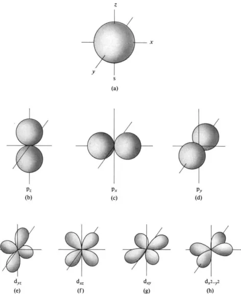
The rules for placing further electrons around a nucleus developed as the Bohr theory was applied to atoms other than hydrogen. First, it was necessary to allow elliptical as well as circular orbits, whose angular momenta were quantized. The wave mechanical treatment (see Section 16-7) leads naturally to this second quantum number £, called the azimuthal or angular quantum number, and further specifies that for a given η, £ can have the values 0, 1,..., η — 1. As a consequence of early descriptive assignments by spectroscopists, these £ states are often designated s (sharp), ρ (principal), d (diffuse), and f (fundamental), referring to

£ = 0, 1, 2, and 3, respectively (beyond this, the lettering is alphabetical: s, p , d, f,g, h , i , j , . . . ) .

Second, the observation of splitting of spectral lines in a magnetic field (called the Zeeman effect) led to another quantum number m, called the magnetic quantum number, which gives the possible projections of the orbital angular momentum in the direction of the field. Again, the magnetic quantum number appears natu­

rally in the wave mechanical treatment, which specifies that m can have the integral values —£, —(£ — 1), 0 , £ — 1, and £, or a total of 2£ + 1 values in all.

Finally, the discovery of electron spin led to the introduction of a fourth quantum number, the spin quantum number 0 , whose value can be \ or — \ , the angular momentum of the spinning electron being ο(Η/2π).

16-3 HYDROGEN AND HYDROGEN-LIKE ATOMS 663

The first few possible combinations of these four quantum numbers are as follows:

0(s) m = 0 _{o = h - i} ί = 0(s) m = 0 _{o = h - i} ί = 1(Ρ) ^{m =} —1

- \

m = 0 _{o = \ ,} ~\

m = 1 _{o = h} ~\

0 ( s ) m = 0 ~\

ί = 1(Ρ) ^wi = —1

' = i,

m = 0 < = h ^{_ I} 2

<m = 1 _{o = h} ¹ ₂

ί = 2 ( d ) <m = —2

- \

m = —1 _{o = h}

- \

m = 0 _{o = h}

- \

Ml = 1 _{o = h}

- \

<m = 2 _{ο = h}

-\.

Experimental spectroscopy led Pauli (1925) to conclude that no two electrons may have the same four quantum numbers. By this Pauli exclusion principle only 2 electrons can be in the η = 1 state, 8 in the η = 2 state, 18 in the η = 3 state,

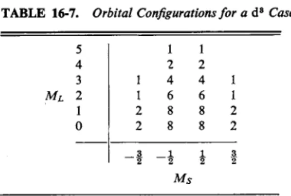
T A B L E 1 6 - 1 . Ionization Energies

Ionization energy / for successive electrons (a.u.) Outer electron

Element Ζ configuration A h h h h

Η 1 Is 0.50

H e 2 I s² 0.90 2.00

Li 3 l s²2 s 0.20 2.78 4.5

Be 4 ...2s² 0.35 0.67 5.65 8.0 — — — —

Β 5 ...2s²2p 0.31 0.93 1.4 9.53 12.5 — — —

C 6 . . . 2 s²2 p² 0.42 0.90 1.76 2.37 14.4 17.9 — —

Ν 7 . . . 2 s²2 p³ 0.53 1.09 1.74 2.84 3.60 18.6 24.4 — Ο 8 . . . 2 s²2 p⁴ 0.50 1.29 2.02 2.84 4.18 5.06 27.0 32 F 9 . . . 2 s²2 p⁵ 0.64 1.29 2.30 3.20 4.20 5.75 6.8 35 N e 10 . . . 2 s²2 p^e 0.79 1.51

N a 11 ...2s²2p^e3s 0.19 1.74 2.62

M g 12 ...3s² 0.28 0.55 2.95 — — — ^-— —

Al 13 ...3s²3p 0.22 0.69 1.05 4.41 — — — —

Si 14 . . . 3 s²3 p² 0.30 0.60 1.23 1.66 6.12 — — —

Ρ 15 . . . 3 s²3 p³ 0.41 0.73 1.11 1.89 2.39 — — —

S 16 . . . 3 s²3 p⁴ 0.38 0.86 1.29 1.74 2.66 3.22 — —

CI 17 . . . 3 s²3 p⁵ 0.48 0.88 1.47 2.00 2.50 3.56 4.18 —

Ar 18 . . . 3 s²3 p^e 0.58 1.02 1.51 2.20 — — — — Κ 19 ...3s²3p^e4s 0.16 1.17 1.75

Ca 20 ...4s² 0.23 0.44 1.88

Sc 21 ...4s²3d 0.24 0.48 0.91 2.72 — — — —

Ti 22 . . . 4 s²3 d² 0.25 0.50 1.04 1.59 3.67 — — —

V 23 . . . 4 s²3 d³ 0.25 0.52 1.09 1.79 2.35 4.88 — —

Cr 24 ...4s3d⁵ 0.25 0.61

M n 25 ...4s²3d⁵ 0.28 0.58

and so on, For example, the ground- or lowest-energy state of Li has the electron configuration ls²2s, the first number denoting the principal quantum number and the superscript the number of electrons of the indicated £ value. Table 16-1 lists the outer electron configurations for a number of elements, along with their energies for the ionization of successive electrons.

We can now proceed with some further examples of Z^ett calculations. The first ionization energy for Li is 0.20 a.u., and since η = 2 for this electron, Eq. (16-19) gives Zeff = [(0.20X2X2)²]¹/² = 1.26. For N a the outer electron is 3s and its ionization energy is 0.19 a.u., giving Z^eff = 1.85 as compared to the actual Ζ = 11.

It requires 1.75 a.u. to remove a second 2p electron, however, and now

Z^{e f f} = [(1.75)(2)(2)²]¹/² = 3.7. Thus the electrons in the η = 2 shell of N a are

exposed to about one-third the full nuclear charge. The difference between Ζ and Zeff is called the screening constant s. This constant is 7.3 for N a⁺ and 9.15 for Na, for example.

The Bohr model encountered increasing difficulties as attempts were made to apply it to atoms other than hydrogen; furthermore, it failed to account for the de Broglie principle that particles behave as though they had characteristic wave­

lengths. The de Broglie hypothesis was quantitatively confirmed by the second half of the 1920's through experiments, such as those of C. Davisson and L. Germer and G. Thomson, that showed that electrons produce x-ray-like diffraction patterns on striking a gold foil. The hypothesis is also consistent with the Heisenberg uncertainty principle that the position of a particle cannot be stated exactly but only as a probability. A new model was needed that would unite all the aspects of the behavior of atoms and electrons; this was provided in 1926 by E. Schrodinger and W. Heisenberg, somewhat independently.

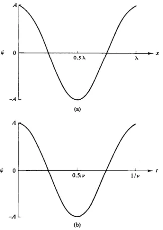
Schrodinger used the mathematical framework that had been developed for periodic motions such as those of waves. For a plane wave of electromagnetic radiation, the classical equation is of the form

where Ψ is the amplitude of the wave at point χ and time r, λ is its wavelength and ν is its frequency; the constant A determines the maximum amplitude. Equa­

tions of the form of Eq. (16-20) will appear frequently in the following material and an important identity to keep in mind is

(as one can verify by writing out the respective series expansions). Equation (16-20) may be written as

16-4 The Schrodinger Wave Equation

(16-20)

e±ix __ CQS x 4- I sin χ (16-21)

(16-22) The intensity of a wave is given by the square of its amplitude, and if the latter is complex, by ΨΨ*, where Ψ* is the complex conjugate of Ψ, in this case

16-4 THE SCHRODINGER WAVE EQUATION 665

FIG. 16-2. The amplitude of a wave, (a) As a function of distance at a given time and (b) as a function of time at a given position.

A exp[—2m(x/X — vt)]. By using Eq. (16-22), we can see that the intensity for a plane wave is just A². Also, by using the real part of Eq. (16-22), we can plot amplitude as a function of χ and this is just a cosine function oscillating between A and — A, with a wavelength λ if plotted against χ with t constant, or of frequency ν if plotted against time with χ constant. Figure 16-2 shows such plots.

Equation (16-20) is a solution to the second-order partial differential equation (16-23) where υ is the velocity Xv of the wave, as one can verify by carrying out the differen­

tiations. One may then put the corpuscular nature of light quanta into Eq. (16-23) by replacing λ by h/p [Eq. (16-7)] and ν by e/h [Eq. (16-2)], whence Xv = e/p:

(16-24) The next step is to restrict the situation to standing waves, that is, waves whose amplitude at a given J C is not a function of time. This is done by writing Eq. (16-20) as

(16-25)

One then deals only with the φ function, for which the differential equation is

= (16"26)

(obtained by differentiating φ = Ae^2nix^ twice and replacing λ by hip).

Schrodinger modified equations of this type to apply to a particle. The kinetic energy of a particle is \mv², or p²/2m, and kinetic energy can be regarded as the total energy Ε minus the potential energy V. On substituting p² = 2m{E — V) into Eq. (16-26), one obtains

ά²φ %π²ιη ^{ί τ 7} - , Λ

or

h² ά²φ

%π²ηϊ dx² + νφ = Εφ. (16-27)

Equation (16-27) is the Schrodinger wave equation in one dimension for a particle which is present as a standing wave. By hypothesis, the energy of the particle is given by E, and the probability of finding it between χ and χ + dx is given by φ*φ dx. Generalization to three dimensions gives

If qne does not wish to specify a particular coordinate system (such as the Cartesian one used here), one writes the equation in the form

h* ν²φ + Υφ = Εφ, (16-29)

87r²m

where V² is known as the Laplace operator, del squared. It is then necessary to derive the detailed expression for V² for each new coordinate system, as, for example, the polar one that is used in Section 16-7. A yet more concise form is

Ηφ = Εφ, (16-30) where Η stands for the operations on φ called for by the left-hand side of

Eq. (16-29). This is known as the Hamiltonian operator (of wave mechanics), so named by analogy with a similar function that appears in the classical equations of motion.

Schrodinger pursued the analogy to classical wave equations further by postu­

lating the more general equation

h² h 8Ψ

- ^ V " V

^ +

$π²ιη 2πι dt

where Ψ is a function of both position and time. As was done with Eq. (16-25), we assume the special case in which Ψ can be written as a product φφ, where φ is a function of time alone (and φ has already been taken to be a function of position alone). If this substitution is made into Eq. (16-31), then V²W becomes φ ν²φ (since φ is not a function of coordinates) and θΨ/dt becomes φ δφ/dt

16-4 THE SCHRODINGER WAVE EQUATION 667 (since φ is not a function of time). On dividing through by φφ⁹ we obtain

The left-hand side of Eq. (16-32) is a function of coordinates only [assuming that V Φ/(/)] and the right-hand side is a function of time only; consequently the quantity to which both sides are equal cannot be a function either of time or of coordinates—it must be a constant. Another way of phrasing one of Schrodinger's hypotheses is to say that we take this constant to be E⁹ the total energy. Equation (16-32) then separates into two equations, Eq. (16-29) and the time-dependent equation

άφ _

-αψ--ΊΓ

>

which integrates to

φ =

This is the same as Eq. (16-33) if we write Ε = hv. Remembering relationship (16-21), φ is evidently a function which oscillates with time.

Nearly all of the applications of wave mechanics treated in this text will be in terms of φ rather than Ψ. The typical application of Eq. (16-29) will be to an electron under the influence of some potential V, usually a potential well. In the case of the hydrogen atom, for example, V = —e²/r. The solutions to Eq. (16-29) then give the various energies which an electron can have if it is to act as a standing or stationary wave. Such a stationary state is possible only for certain wavelengths, depending on the nature of V⁹ and hence only for certain energies. It will turn out, in other words, that discrete or quantized energy states appear as a natural conse­

quence of our asking for stationary solutions to the wave equation. The stationary- state solutions are the appropriate ones for an atom or molecule which does not change with time. Rate processes, such as the emission of radiation (fluorescence), require the use of the full equation, (16-31), a use which is largely beyond the scope of this text; see, however, Section 19-ST-l.

A remaining point is that while Eq. (16-29) is the wave equation for a single particle, in this case, an electron, obeying a potential energy function V and having total energy E, there is a simple recipe for constructing the wave equation for a system of particles. The first term of Eq. (16-29) plays the role of the kinetic energy of the particle and if more than one particle is involved, an analogous term is written for each of them. That is, the first term becomes Σ< ~~ [{h²l%TT²m^ ^²φ]

if i particles are present. Then V becomes the function giving all the mutual interactions between the particles; Ε is still the energy of the system.

Further comments are the following. Equation (16-27) was obtained from the equation for a wave by replacing λ by h[p and using the statement of energy con­

servation:

total energy = kinetic energy + potential energy

Ε p²\2m(pt\mv²) V. (16-34)

Alternatively, one may take as a postulate of wave mechanics that in Eq. (16-34) momentum, p⁹ is replaced by (h[2m)(dldx)⁹ and total energy, E⁹ by — (λ/2ττ/)(3/3ί).

These replacements are operators; they carry instructions to differentiate. Equation

(16-31) results if, after the substitution, each term is multiplied by Ψ, the function to be operated on. It is postulated that the product Ψ*Ψ (or φ*φ) gives the prob­

ability of finding the particle at each point in space.

Characteristically, the wave equation is solved subject to some set of restrictions.

In each of the situations that we take up in this chapter, for example, we will require that φ be everywhere continuous and single-valued. In addition, the solu­

tion must obey certain boundary conditions. Typically, φ should go to zero at large x; we may require it to be angularly periodic. We will see that it is these boundary conditions that restrict integration constants to integral values—values that turn

out to be quantum numbers.

In concluding this section, it should be emphasized that while the Schrodinger equation can be obtained by means of certain analogies with classical wave equa­

tions, there does not exist a rigorous derivation. The Schrodinger equation is taken to be correct by hypothesis, and therefore is itself the starting point of wave mechanics. The various analogies are useful in trying to attach some physical picture to the solutions obtained; they are also dangerous because wave mechanics does not rest on a physical picture (as does the Bohr theory)—it is a purely mathematical model [see Bridgman (1961)].

16-5 Some Simple

Choices for the Potential Function V

A. The Free Particle

One of the simplest applications of the Schrodinger wave equation is to a particle for which the potential function is a constant. It is customary to take V = 0; if V has some other value, it merely shifts the energy of the system accord­

ingly. Equation (16-28) therefore becomes

h² (32φ θ²φ 3²φ\

" ( a F -

-ψ

7*1

"

or

Η^χφ + Η^νφ + Η^ζφ = Εφ. (16-36) Any wave equation such as Eq. (16-36), in which Η can be written as a sum of

terms that do not share coordinates, can be resolved into the set

Η^χφ^χ = Ε^χφ^χ , Υί^νφ^ν = Ε^υφ^ν , Υί^ζφ^ζ = Ε^ζφ^ζ, (16-37) where φ = φ^χφ^υφ^ζ and Ε = Ε^χ + E^y + Ε^ζ. The procedure for demonstrating this conclusion is entirely analogous to that used in obtaining Eqs. (16-32) and (16-33). One substitutes φ^χφ^υφ^ζ for φ in Eq. (16-35) and then divides through by φ^χφ^υφ^ζ. The left-hand side then consists of a sum of terms in χ only, y only, and ζ only, and therefore separates into the three equations (16-37).

In the present case, the x, y, and ζ equations are identical in form, so that only

16-5 SOME SIMPLE CHOICES FOR THE POTENTIAL FUNCTION V 669

6. The Particle in a Box

We may next stipulate that the particle has zero potential energy over a region defined by 0 < χ < a, 0 < y < b, and 0 < ζ < c, but that beyond these bounda­

ries the potential energy is infinite. That is, V^x is zero for 0 < χ < a and is infinite for χ < 0 and χ > a, and similarly for V^y and V^z ; hence the term " b o x . " Equa­

tion (16-28) is now

The situation is the same as for Eq. (16-35) in that the substitution φ = φ^χφ^νφ^ζ allows the equation to be separated into three separate ones:

- — ^ + ν.φ. = Ε^χφ^χ (16-43)

%7T²m dx²

and similarly for y and z, where V = V^x + V^y + V^z and Ε = E^x + E^y + E^z. Alternatively, Eq. (16-43) may be viewed as the wave equation for a particle in a one-dimensional box.

The solution to Eq. (16-43) is the same as that for Eq. (16-38) for the region inside the box, since V^x = 0. However, the solution outside the box, where V = o o , must be that φ^χ = 0. This conclusion can be reached on both physical and mathe- one need be solved:

h² dH*

" W a s ? =

"

A stationary-state solution to Eq. (16-38), that is, one for which Ε is not a function of time, is

. . . [ 7 %π²ηιΕ^χ \ V 2 -,

0^Β = Λ « η [ ( x\, (16-39)

as we can verify by substituting back into Eq. (16-38); A^x is an integration con­

stant (note Problem 16-4). Since the wave is not confined, there are no restrictions on its wavelength and E^x can have any positive value. The total φ is then the pro­

duct

, ^A . [γ 8n²mE^x \V² ι . \/Sn²mE^y\^² ι . \/^²mE^z\^² ι ^{n c} ,^m φ = Α*ιη[( ^{h 2} *) x\sm[[ ^ ^y) y\ s i n [ ( j^-) z\ (16-40)

and corresponds to an infinite sinusoidal wave in three dimensions.

The wavelength in, say, the χ direction is given by

λ = (WmEJh^ ' ^{( 1 6}"^{4 1 )}

since for this value of χ we have sin 2π, which completes one cycle. Equation (16-41) simplifies to λ = hj{2mE^xyi², but E^x is also equal to p^x2/2m, so the final result is just the de Broglie equation, λ = h/p. This result is not too surprising in view of analogies made when writing down the wave equation.

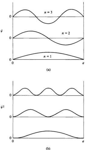
FIG. 16-3. φ and φ² functions for a particle in a one-dimensional box.

matical grounds. Physically, it should be impossible for the particle to escape the box, and since φ^χψ^χ* dx gives the probability of finding the particle in the region dx at each x, it follows that φ^χψ^χ* = 0 and hence ψ^χ = 0 for χ < 0 and χ > a.

The mathematical reasoning is that the curvature of the plot of ψ^χ versus x, 8²φ^χ/3χ², is proportional to (V^x — E^x) φ^χ ; if V^x = oo and φ^χ φ 0, then the curvature must be infinite and φ^χ must increase to infinity itself. This is an impos­

sible catastrophe—it is not acceptable that φ^χ, and hence the probability function for the particle, be infinite anywhere. This catastrophe can be avoided only if φ^χ is zero (and hence the curvature is zero) for χ < 0 and χ > a.

We also do not expect φ^χ to change discontinuously, that is, to have two values at a given x. There should be only one probability for the particle being at any one position. Since ψ^χ must be zero just outside the box, it must therefore also be zero just inside the box. The consequence is that only those values of E^x in Eq. (16-39) are acceptable which make φ^χ zero at χ = 0 and at χ = α, which means that the wave must have a node at these boundaries. In other words, there must be an integral number n^x of half-wavelengths in the distance a, as illustrated in Fig. 16-3. As applied to Eq. (16-41), the condition is that a = η^χλ/2, or, on rearrangement,

h²n ²

£* = CT> " , = 1 , 2 , 3 , . . . . (16-44)

16-5 SOME SIMPLE CHOICES FOR THE POTENTIAL FUNCTION V 671

Also, substitution of this expression for E^x into Eq. ( 1 6 - 3 9 ) gives

φ^χ = Α^χ*ίη(?ψ-). ( 1 6 - 4 5 )

One further step is usually taken with a solution to the wave equation. The solution will contain a constant of integration, A^x in Eq. ( 1 6 - 4 5 ) , and the value of A^x is usually set so that the probability of the particle being somewhere is unity.

The function is then said to be normalized. In the present case this condition is

j φ^χψ^χ* d r = \ = A* J ° [sin(^i-)]² dx, ( 1 6 - 4 6 )

where the first integral is the formal statement that the integral of ψ^χφ^χ* over all space is to be unity and the second integral is the specific one involved here.

The integral is a standard one, equal to a/2 for the given integration limits. The constant A^x is therefore (2/a)¹/² and the normalized solution is

The preceding illustrates a fairly typical procedure in obtaining wave mechanical solutions. One uses the requirement that φ be everywhere finite and single-valued if the solution is to have physical meaning, and this requirement then limits the possible number of solutions and hence of energy states. Quantization thus appears naturally and not as an ad hoc assumption.

To continue with the particle-in-a-box treatment, we see that the solutions for the y and ζ coordinates are the same as that for the χ coordinate, so the complete solution for a three-dimensional box is

and

where, for generality, the x, y, and ζ dimensions of the box are taken to be a, b, and c, respectively. Alternatively, for a two-dimensional square and a three- dimensional cubic box,

h² Sma²

^square = " ό — F ("*² + V ) > (16-50)

£cube = g^r("a? + η ² + η²). (16-51)

C. Some Applications

The equations for the particle in a box have several important applications.

One of these is the use of Eq. (16-51) to supply the energy states for a gaseous molecule in a container of volume V, thereby leading to the translational partition function for an ideal gas (see Sections 4-10 and 6-9C). The spacing of these energy states is quite small if the side a is of macroscopic size or if the particle is massive.

On insertion of numerical constants, Eq. (16-44) becomes (6.6256 X 10-")2(6.0225 χ 10»«χΐ0") n^x*

8 Λίά²

2 2

= 3.305 χ 1 0 "1 4 J*T-2 (erg molecule"1) = 476

jfa

The spacing becomes quite respectable, however, for a light particle such as an electron in a box of atomic dimensions. The atomic weight of the electron is 0.000549 g mole" \ so that Ε is

E = S61^4 kcal m o l e "¹ = 303 % • k K = 3 7 . 6 % ' eV. (16-53)

a2 a2 a2

Equation (16-53) may be applied in an approximate treatment of certain types of molecules which have electrons that can oscillate over the whole structure.

The electrons which form the double bond in ethylene probably behave in this way. A more interesting example is butadiene, H2C = C H — C H = C H2, in which each carbon atom contributes one electron to the double bond system, and these four electrons probably can oscillate over the entire length of the chain. That is, the double bonds are not really localized to the particular pairs of atoms shown.

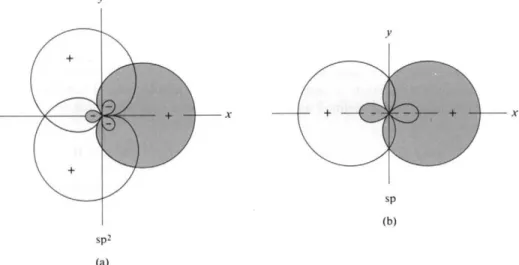
In effect, then, the four electrons are in a one-dimensional box equal in length to that of the chain. This last can be estimated as equal to two C = C bond lengths or 2(1.35) A, plus one C—C bond or 1.54 A, plus the distance of a carbon atom radius at each end or another 1.54 A, for a total of 5.78 A. Equation (16-53) then gives the energy states in eV as [37.6/(5.78)2]«Λ.2 = 1.12Λ*². By the Pauli exclusion principle, each state can hold two electrons (with spins opposed), and so the four electrons fill the first two levels as illustrated in Fig. 16-4(a).

The energy of the first excited state of this system of four electrons is that for having one electron in the η = 3 level, and the energy to produce this state is Ε = 1.12(3² - 2²) = 5.60 eV or 45,000 c m -¹. Butadiene does have an absorption band at 46,100 c m- 1 (217 nm), and the very simple free-electron model, as this is called, has been fairly successful.

As a further example, hexatriene, H²C = C H — C H = C H — C H = C H², should have six delocalized electrons in the double bond system, in a box of length 8.67 A.

The energy for the η = 1 state is then 37.6/(8.67)2 = 0.500 eV, and as shown in Fig. 16-4(b), the six electrons fill the first three levels. The first excited state should now have one electron in the η = 4 state, and Δ Ε for the transition should therefore be 0.500(4² - 3²) = 3.50 eV or 28,000 cm"¹. The experimental value is 38,500 cm"¹, and although the agreement is rather poor, the model has correctly predicted that the frequency of the absorption band should decrease with increasing chain length.

The free-electron model is a semiempirical one—one does not know, for example, just how much "end space" to allow in calculating the length of the box. The uncertainty becomes less important with longer chains, and with carotene, which has alternating single and double bonds in an 11 carbon atom chain, one estimates about 25,000 c m- 1 for the transition to the first excited state, as compared to 22,200 c m- 1 observed. The model may also be applied to two-dimensional boxes,

16-6 THE HARMONIC OSCILLATOR 673

η = 3 10.08 eV

η — 1 4.48 eV

« = 4

n = 3

8.00eV

4.50eV

η — 2 2.00 eV η = 1 0.50 eV η = 1 1.12 eV

ι

(a) (b) F I G . 1 6 - 4 . Particle-in-a-box energy level scheme for (a) butadiene and (b) hexatriene.

such as benzene or fused aromatic ring systems, with Eq. (16-50). A more sophisticated treatment is given in Section 18-7.

It may happen that two or more solutions to the wave equation for a system have identical energy. Such solutions and the corresponding states of the system are said to be degenerate. Consider, for example, a two-dimensional box for which the energy states are given by Eq. (16-50). The energy for a state {n^x = 1, n^y = 2) is identical to that for a state (n^x = 2, n^y = 1) and the state of this energy is said to be doubly degenerate.

16-6 The Harmonic Oscillator

The harmonic oscillator represents the simplest possible model for an atom vibrating in a potential well. The force on the atom is in this case —ix, that is, proportional to the displacement χ from the equilibrium position, and is negative since it is a restoring force. The potential energy is then \dx², corresponding to the parabolic curve in Fig. 16-5, and the wave equation is

S + ^ ( * - ^ = 0. (16-54)

F I G . 1 6 - 5 . The potential en- ergy function for a harmonic oscillator.