The output employment elasticity and the increased use of temporary contracts: Evidence
from Poland
KRISTOF BARTOSIK
1pand JAN MYCIELSKI
21Institute of Economics of the Polish Academy of Sciences, Nowy Swiat 72, 00-001, Warsaw, Poland
2Faculty of Economic Sciences, University of Warsaw, Poland
Received: December 18, 2017 • Revised manuscript received: August 16, 2018 • Accepted: April 3, 2019
© 2020 Akademiai Kiado, Budapest
ABSTRACT
The paper investigates how the increased use of temporary contracts in Poland affected employment elasticity with respect to output. The analysis is based on Okun’s law, and covers the period of 1996–2016, with particular focus on the years of 2001–2016 when temporary jobs became prevalent. We look at the relationships between output growth and the growths of aggregate, permanent and temporary employment separately. Our study finds that the responsiveness of aggregate employment to output is positive and changes through time. Interestingly, after 2007, when the use of temporary contracts stabilised at a high level, the employment intensity of growth started decreasing. We relate this to the opposite trends in output responsiveness of temporary and permanent jobs. Elasticity of temporary job was growing, while elasticity of permanent job was decreasing. Our study also shows that initially employers adapt to output changes replacing permanent job with temporary job, next temporary contracts become the main adjustment device.
KEYWORDS
Okun’s law, labour demand, temporary contracts, economic growth JEL CLASSIFICATION INDICES
J21, J23, E32, J41
pCorresponding author. E-mail: kbartosik0303@gmail.com
1. INTRODUCTION
Understanding the determinants of employment intensity of growth, particularly the reasons for the differences in this intensity across countries and over time, is important for policy makers.
The aim of this paper is to explore whether and to what extent the increased use of temporary contracts has affected output elasticity of employment in Poland.
Studying the Polish case is interesting for at least two reasons. First, Poland experienced significant changes in the employment structure. Between 2001 and 2005 the share of temporary workers in total employees soared from 12 to 26% and fluctuated between 26 and 28% in the following years (Figure 1). At the same time the share of temporary workers in employment rose from 6% to 20–22%. Thus, the share of this type of workers in the labour force has reached the highest level in the EU.
Second, there seems to be a contradiction between the Polish empirical data and common view on the influence of the widespread use of temporary contracts. According to this view, the high share of temporary workers plays an important role in the increase in employment responsiveness. For this reason, compared to permanent workers, temporary workers offer advantages in terms of flexibility and costs, i.e. they provide for shorter notice periods and lower severance payments, and exhibit greater responsiveness to output fluctuations.
Previous studies confirmed that the incidence of temporary jobs affects employment or unemployment sensitivity to output changes. These studies can be divided into two groups. The first group consists of papers analysing the effects of two-tier (partial) reforms of labour markets.
These reforms are intended to increase job creation and to cut unemployment by easing the use of temporary contracts, but keeping existing protection for permanent workers. A number of papers look at Spain, where the two-tier reform resulted in the share of temporary workers reaching 35% of employees in 1990s. These papers are based mainly on labour demand model or search and matching model, which allows for two types of contracts–permanent and temporary and examines how difference in firing costs affects labour demand. According to Bentolila – Saint-Paul (1992), temporary contracts increased the cyclical response of employment in the Spanish industrial sector.Costain et al. (2010) showed that unemployment is more volatile in
Figure 1.Share of temporary workers in total employees in Poland, Spain and EU (27) (%, 1995– 2016).Note: Quarterly data, seasonally adjusted.
Source: Eurostat, Polish LFS and own calculation.
84 Acta Oeconomica70 (2020) 1, 83-104
labour market with permanent and temporary contracts, than in the labour market with a single contract type.Bentolila et al. (2012)found that the larger difference between thefiring costs of permanent and temporary workers in Spain than in France, which, to a great extent, explains why unemployment rate increased more in Spain than in France during the financial crisis.
Jimenez-Rodriguez–Russo (2012)claimed that the partial labour market reforms increased the output employment responsiveness in France, Germany, Italy and Spain, and made them comparable to that in the UK.
Another important lesson from these studies is that the gap in separation costs has an ambiguous effect on average employment. This is because the gap, on the one hand, encourages employers to hire, on the other hand encourages employers to substitute temporary for per- manent contracts. According toBentolila–Saint-Paul (1992) and Boeri–Garibaldi (2007), the two-tier labour market reforms transitionally increase employment. Also,G€uell (2003), Kahn (2010), Cahuc et al. (2016) and d’Agostino (2018) reported that the gap in dismissing cost increases the share of temporary jobs, but has a negligible effect on employment.
The second group of papers analysing the effects of temporary contracts includes analyses on macro level revisiting Okun’s law.1IMF (2010), Boeri (2011)andDixon et al. (2016)confirmed that in many OECD countries increase in the unemployment sensitivity to outputfluctuation is associated with more widespread use of temporary contracts. In turn, Ball at al. (2012) and Cazes at al. (2013)showed that the Spanish Okun’s coefficient is the highest among the analysed countries. As for the research methods,IMF (2010)used the share of temporary employment as the explanatory variable in the long term“dynamic beta”equation, whileDixon et al. (2016) used it in the Okun’s equation. In contrast,Boeri (2011)estimated the Okun’s coefficient (for unemployment and employment) using rolling regression, and compared the responsiveness of employment before and after the two-tier reforms.
The Polish case is under-researched, but so far, the results only partially support the prev- alent view. More precisely, theSocial Diagnosis Report (2015: 136) confirmed that temporary jobs are not as steady as permanent jobs. Over the period of 2009–2015, probability of becoming unemployed was about three times higher for temporary workers than for permanent ones. An empirical analysis of the impact of the growing use offlexible work contracts was presented by Cichocki et al. (2015). They did notfind evidence that the growing use of non-standard labour contracts (includingfixed-term contracts) had resulted in an increased employment elasticity with respect to GDP growth.
Our research extends this literature. First, our study is based on Okun’s law, however in contrast to others studies revisiting the law, we look at the relations between GDP growth and aggregate, permanent and temporary employment growths. Elasticities of employment under different types of contracts are estimated separately and compared. Second, to estimate and analyse these elasticities we use several econometric tools such as Ordinary Least Squares (OLS), Fully Modified OLS (FM-OLS) structural stability tests, rolling regressions, Granger causality test and Markov switching regression. These are in contrast with the analysis byCichocki et al.
(2015)using the Impulse Response Function based on Vector Autoregressive models to estimate the responsiveness of employment to changes in GDP growth across sectors.
1Okun (1962)found an empirical positive relationship between output and employment, and negative relationship between output and unemployment rate.
The analysis in this paper covers the period of 1996–2016, with particular attention paid to the years of 2001–2016, when changes of the share of temporary workers in employment were the most pronounced. Empirical analysis based on the quarterly data.
Our main finding is that the aggregate employment responsiveness to output changes over time, and that over the period of prevalence of term contracts (2006–2016) the responsiveness of employment declined due to the opposite trends in elasticities of permanent and temporary employment. The share and elasticity of temporary employment increased, but the elasticity of permanent employment, which had a dominant share in employment, decreased and, conse- quently, aggregate elasticity decreased as well. These opposite trends also reflect the changes of the way in which labour demand adjusts to output fluctuations.
The paper is organised as follows. Section 2 presents size and structure of temporary employment in Poland. Section 3 shows the theoretical background and data. Section 4 contains empirical research. Section 5 concludes the article and offers some policy recommendations.
2. TEMPORARY EMPLOYMENT IN POLAND, 1996 – 2016
In this paper the term temporary employment(also jobs, workers, and contracts) refers to the category of temporary job adopted by the Polish Labour Force Survey (LFS). In turn,aggregate or total employment refers to dependent employment, and covers both permanent and tem- porary job. In LFS terminology, the category oftemporary jobincludes several types of contracts regulated by the Polish Labour Code and the Polish Civil Code, which differ significantly in terms of employment protection. However, the LFS time series does not inform about structure of temporary employment by forms of contracts, other data sources can shed light on this issue.
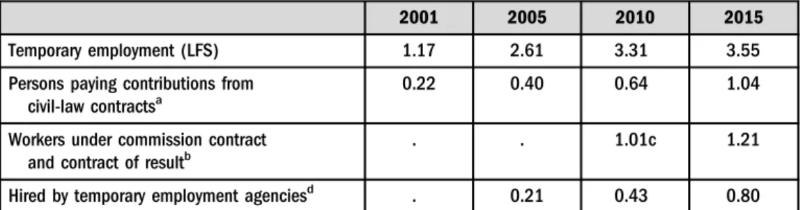
Table 1 provides some information on the size and structure of temporary employment.2 The Labour Code contracts account for approximately 2/3 of the temporary employment. These
Table 1. Increase in temporary employment by different form of contracts (millions)
2001 2005 2010 2015
Temporary employment (LFS) 1.17 2.61 3.31 3.55
Persons paying contributions from civil-law contractsa
0.22 0.40 0.64 1.04
Workers under commission contract and contract of resultb
. . 1.01c 1.21
Hired by temporary employment agenciesd . 0.21 0.43 0.80
Note: a- excluding contract of result,b- the only source of income,c- in 2012;d- this group includes both workers under civil code and labour code contracts.
Sources:MRPiPS (2016: 29),CSO (2016, Table 15), LFS, SII.
2More details can be found about the development of temporary employment in Poland in e.g.Lewandowski–Magda (2017), Lewandowski (2018).
86 Acta Oeconomica70 (2020) 1, 83-104
contracts included (until 2016): contracts for a fixed period, for a trial period, contracts to complete a specified task and replacement contract (to replace an employee on e.g. maternity leave). Such contracts provide the same working conditions and social benefits as permanent contracts, e.g. sick leave, maternity leave and minimum wage but they can be terminated without a justification (necessary in the case of permanent contracts) and until 2016 notice period was substantially shorter than for the permanent contracts. Thanks to thisflexibility, they were used extensively.
Civil law contracts account for roughly 1/3 of the temporary employment, although the use of civil contracts is restricted by the Polish law. The most popular forms of the civil law contracts are commission contracts and contracts of result. They do not guarantee rights provided by the Labour Code, e.g. sick leave or maternity leave, paid vacation, severance payment, notice period, as well as minimum wage (the last problem was partly eliminated by regulatory changes in 2016). For this reason, civil contracts offer a substantially lower tax wedge. The substitution of a permanent contract with a civil law contract, on the one hand, reduced social contributions, and on the other hand, increased the worker’s net income (Arak et al. 2014). These also make such contracts attractive both to firms and to workers. Civil contracts are predominantly used by employers to cut labour costs or to increase salaries of low-skilled workers. Indeed, workers under civil contracts are paid less on average than permanent workers. For instance,Gatti et al.
(2014)report 15% wage gap, and that roughly 20% of the temporary employment with civil contracts had earnings below the minimum wage.
Table 1reports that the use of temporary contracts was growing rapidly. Contracts under the Civil Code grew considerably faster than contracts under the Labour Code. This expansion was not associated with any substantial changes in regulations. Unlike other countries with high share of temporary contracts, in Poland there was not any two-tier (partial) reform of labour market3. In Poland, the expansion resulted from the interaction of the changes in interpretation and enforcement of the existing law with the difference in employment protection between various types of contracts, and the pressure exerted on labour market by high unemployment.
Various types of term contracts had existed in the Polish law long before their share in total employment rose radically. The most common types of civil contracts, i.e. commission contracts and contract of result were introduced in the 1960s. Over the period of 2001–2005, there were only minor changes in the law that cannot explain the increased use of the term contracts. In 2002, a contract of replacement was introduced, in 2003 unlimited renewal of the fixed contracts were allowed, but this regulation was renounced the next year. After the EU accession in 2004, only two fixed contracts were allowed, next contract had to be open-ended contract. This suggests that the interpretation and enforcement of regulation were changed rather than the legal framework.
Asymmetry in protection between the temporary and permanent workers, which explains the spreading of temporary contracts, existed since the beginning of 1990s. OECD (2004) showed that this asymmetry reinforces the labour market duality, since it encourages the em- ployers to hire workers on temporary contracts, and lowers the rate of conversion from term contracts to permanent contracts. The Polish case tends to confirm this. Expansion of thefixed-
3OECD (2004)presents changes in temporary workers legislation across countries at the turn of the century (see e.g. page 74).
term contracts coincided with the greater gap in employment protection, while the share sta- bilization coincided with the smaller gap. OECD Employment Protection Legislation (EPL) strictness index (see EPL timeseries4) for permanent workers was 2.23 and was constant over the period of 1990–2013. In contrast, the temporary workers index was significantly lower and its volatility reflected changes in the regulation (mentioned above). In the years of 1990–2002, it was equal to 0.75, then the index temporally decreased to 0.25 in 2003, andfinally, after Poland’s accession to the EU in 2004, it rose to 1.75 and was stable in the years to follow.
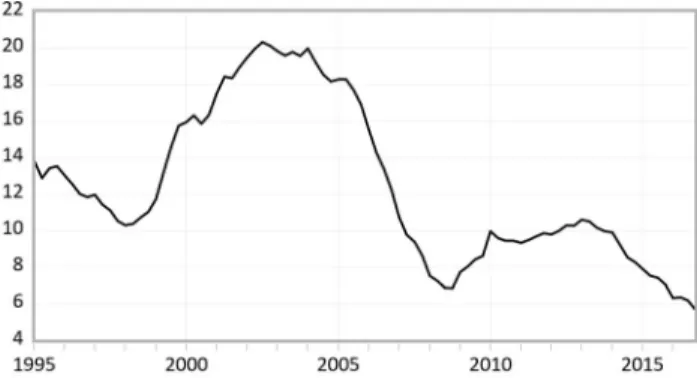
Another factor behind the growth of temporary employment was high unemployment rate which affects the bargaining power of the workers and job seekers and also affects the incidence of temporary contracts. A rapid growth of fixed-term contracts between 2001 and 2005 took place when unemployment rate soared to almost 20% due to the increase in supply of new workers related to the demographic wave and the economic slowdown. The share of temporary employment stabilised after the EU accession, when economic recovery and emigration to the EU countries decreased unemployment rate more than twice (Figure A1inAppendix A). This suggests that both changes in the labour demand and labour supply contributed to the spreading of temporary jobs.
These were the main factors that transformed the Polish labour market into a dual market.
The first segment consists of workers under permanent contracts who are strongly protected by law. The second segment consists of workers under various forms of term contracts. The use of temporary workers is eased and becomes relatively cheaper compared with the permanent workers.
In the following sections we examine how this segmentation affects the output respon- siveness of labour demand.
3. MODEL AND DATA
As in the seminal paper byOkun (1962), we assume that outputfluctuations causefirms to hire and fire workers. In others words, changes in GDP growth rate or in GDP level affect employment growth rate or employment level. The relation can be written as a “difference” version (1) or“gap”version (2):
Δet ¼b0þb1Δytþ«t (1) ΔetΔe*t
¼b0þb1 ΔytΔyt*
þ«t (2) whereΔrepresents change from the previous period,eis employment,yis output,e* is long- run level of employment,y*is long-run output or potential output,tis time index and«is error term.
We estimate the“difference”versions of the Okun’s law. Eqs. (1) and (2) make it possible to estimate output elasticity of employment (b1) and the“jobless growth threshold”(–b0/b1), i.e.
growth which is slower than the threshold causes employmentfigures to fall, while faster growth causes employment rates to rise. Estimation of Eq. (2) is potentially more problematic because it
4http://www.oecd.org/els/emp/oecdindicatorsofemploymentprotection.htm(access: 22.03.2017).
88 Acta Oeconomica70 (2020) 1, 83-104
uses unobservable variables e* and y*. Different measures of long-run employment and po- tential output can produce different results.
The coefficient (b1) depends on the cost-of-employment adjustment. Firms try to reduce or avoid this cost and, among others,first is fire or hire“cheaper”temporary workers. Therefore, we expect that the output elasticity of temporary employment is higher than that of the per- manent employment, and also, that more widespread use offixed-term contracts has increased the employment elasticity in Poland.
Estimating elasticities, we use logs of original variables as well as the logarithmic growth rates calculated as first order differences of the logs of levels of the original variables. Therefore, the calculated elasticities of labour should be interpreted as a percentage change of employment growth resulting from a 1% change in GDP growth rate. We use quarterly data from the LFS.
Employment statistics come from the LFS database revised by the National Bank of Poland (NBP),Saczuk (2014)and these are based on data published in Quarterly information on the labour marketby the Central Statistical Office of Poland (CSO). Due to lack of data, over the period of 1995–2000 we use a casual worker approximation of temporary workers and calculate the number of permanent workers as the difference between employees and temporary workers.
The data on employment for the quarters of 1999Q2 and 1999Q3 are interpolated. Data for real GDP growth rate before 2003 is taken fromStatistical Bulletinsof the CSO and after 2002–from Poland macroeconomic indicators available on the CSO website. The growth in output and employment is measured as the quarter to the same quarter of the previous year.
4. EMPIRICAL ANALYSIS
4.1. GDP growth and employment growth
Some previous studies suggest that temporary employment is more responsive to output than permanent employment and that widespread use of temporary contracts may affect the responsiveness of aggregate employment to output. We start to investigate this issue calculating the Spearman correlation coefficients of output growth–employment relationship for aggregate, permanent and temporary employment separately. Taking into account the share of temporary employment (Figure 1), the sample period 1996–2016 is divided into three subperiods: 1996– 2000, 2001–2005 and 2006–2016.Table 2presents the correlation coefficients (additionally, in Table 2.Spearman correlation between GDP growth and aggregate, temporary and permanent employment growth
1996–2016 1996–2000 2001–2005 2006–2016
Aggregate 0.48*** 0.41* 0.70*** 0.53***
Permanent 0.38*** 0.32 0.72*** 0.32**
Temporary –0.07 0.29 –0.63*** 0.46***
Note:/***/**/*/indicate statistical significance at the 1, 5, and 10 per cent level, respectively.
Sources:LFS, CSO and own calculation.
Appendix Figure A2 depicts developments of GDP and aggregate employment growth in the sample period). Clearly, the output growth is positively and significantly related to aggregate employment growth. However, the estimated coefficients are different before, during and after the expansion of temporary contracts.
Table 2also suggests that the relationships between GDP growth and growths of temporary and permanent employment exhibit different patterns. In the period of 1996–2000, both per- manent and temporary employment growth were positively related to output growth, however this relation was statistically insignificant. In the period of 2001–2005, when the share of temporary contracts was growing rapidly, the correlation of permanent employment increased substantially, while the correlation of temporary employment became negative. In turn, in the period of 2006–2016, the share of temporary contracts was high and relatively stable and the correlation of temporary employment became positive again, while the correlation of permanent employment dropped.
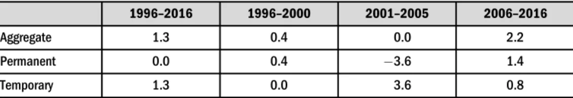
Note that the period of 2001–2005 stands out as the estimated coefficient between temporary employment and output growth is negative and significant. This suggests that the expansion of fixed-term contracts was associated with others factors than GDP growth. According to the cited studies, employers substitute “expensive”permanent workers with “cheap”temporary workers in order to cut labour cost and these substitutions have a negligible effect on aggregate employment. To investigate this, we calculated contributions of permanent and temporary employment growth to aggregate growth.Table 3reports our results. The third column shows that over the period of 2001–2005, when temporary contracts became prevalent, the contri- bution of temporary workers was 3.6 percentage points, while the contribution of workers under open-ended contracts was –3.6 percentage points. Hence, the average rate of aggregate employment growth was at 0.0%. In absolute terms, between the year 2000 and 2005, the number of temporary workers increased by about 1.8 million, whereas the number of permanent workers declined by roughly 1.8 million. As a result, the share of term contracts increased, whereas the number of employees did not increase. In this period, temporary jobs were replacing permanent jobs5. In turn, in the years of 2006–2016 both permanent and temporary contracts contributed positively to aggregate growth, 1.4 and 0.8 % point respectively, and aggregate employment grow at 2.2%.
Table 3.Average quarterly growth rate in aggregate employment (%), and contributions of permanent and temporary employment growth (in percentage points), in selected periods
1996–2016 1996–2000 2001–2005 2006–2016
Aggregate 1.3 0.4 0.0 2.2
Permanent 0.0 0.4 3.6 1.4
Temporary 1.3 0.0 3.6 0.8
Sources:LFS and own calculation.
5This is consistent with the hypothesis that high and persistent unemployment contributes to spreading of term contracts. On the other hand, it cannot be excluded that the substitution of permanent contracts with term contracts is preventing unemployment, by reducing cost and preventing dismissal of some workers.
90 Acta Oeconomica70 (2020) 1, 83-104
These preliminary examinations suggest that: (a) the relationship between output growth and growths in aggregate, permanent and temporary employment was changing over time; and (b) the relationship between permanent and temporary employment growth was also unstable.
We further investigate these issues using econometric methods and the concept of output elasticity of employment.
4.2. Output elasticity of employment
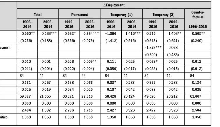
We estimate output elasticity with several econometric tools. The standard and simplest way is to estimate the parameters by the OLS method. We use this method to calculate the static Okun’s coefficients for total, permanent and temporary employment. As the results of the autocorrelation test suggested that a serious autocorrelation problem was present in these regressions, we used the Newey-West autocorrelation robust standard errors for this problem (Table 4).6 The estimated output elasticity for the full sample of total employment is 0.56, while for the subperiod of 2006– 2016 it is 0.59. Both estimates are statistically significant. These results suggest that changes in GDP significantly affect changes in employment, and that the elasticity is slightly higher over the period of widespread use of temporary contracts. However, the difference in the static Okun’s coefficient is small and statistically insignificant. The estimated coefficients (–b0/b1) imply that over the full sample period the GDP growth rate has to be above 1.7% in order to increase employment. However, this estimate is imprecise because of the large variance of the estimated constant termb0, and more extensive interpretation of this value is unwarranted.
The estimated elasticities and the jobless threshold are lower than in the previous studies using the“difference” specification. For example,Czy_zewski (2002) estimated the output elas- ticity of employment for the years of 1993–2000 at 0.7 and the threshold of jobless growth at 3.1%.Ci_zkowicz–Rzonca (2003)reported these measures for the years of 1992–2001, they were equal to 0.9 and 5.7%, respectively.Saget (2000), in her analysis of the transition countries for the years of 1989–1999, got 0.94. The differences between our and estimates cited above are probably the result of different and shorter time series, and suggest that employment intensity of growth has deteriorated in the recent years, while employment threshold has been improved.
Table 4offers a comparison of the output elasticities estimated for permanent and temporary employment. Regressions suggest that the output elasticity of permanent and temporary employment changed over time. Over the full period, a 1 per cent increase in GDP growth is associated with 0.68% increase in permanent employment growth, while over the period of 2006–2016 it is associated with 0.28% change. As for temporary employment, the coefficient is negative and statistically insignificant over the full period, in contrast during the years of 2006–
2016 it is significant at 1.42. These results suggest opposite trends in elasticities and show that compared to permanent employment the output responsiveness of temporary employment was higher over the period of widespread use of term contracts.
Strong autocorrelation of the residuals can result from non-stationarity of the variables included in the regression. We use the Hylleberg, Engle, Granger and Yoo (HEGY) test to check the stationarity of the quarterly growth rates of employment and GDP. The results of the testing are reported in Table B1. For all the series, apart from the series for temporary employment, the null hypothesis of the existence of seasonal and non-seasonal unit roots is rejected at 5%
6We also estimate the“gap”versions of equation, for comparison see Appendix D.
Table 4. OLS estimations for Eq. (1)
ΔEmployment
Total Permanent Temporary (1) Temporary (2) Counter-
factual 1996–
2016
2006– 2016
1996– 2016
2006– 2016
1996– 2016
2006– 2016
1996– 2016
2006–
2016 1996–2016
ΔGDP 0.560** 0.588*** 0.682* 0.284*** –1.066 1.416*** 0.216 1.408** 0.505**
(0.256) (0.188) (0.356) (0.079) (1.412) (0.515) (0.913) (0.621) (0.240)
ΔPerm. Employment –1.879*** 0.028
(0.600) (0.485)
Constant –0.010 –0.001 –0.026 0.009** 0.111 –0.025 0.063* –0.025 –0.012
(0.011) (0.004) (0.022) (0.004) (0.080) (0.017) (0.033) (0.015) (0.012)
N 84 44 84 44 84 44 84 44 84
R2 0.161 0.257 0.138 0.066 0.037 0.283 0.367 0.283 0.134
RMSE 0.025 0.019 0.034 0.020 0.107 0.042 0.088 0.042 0.025
B-G stat. 59.327 21.655 66.321 27.310 58.428 20.124 49.620 20.212 61.667
B-GP-value 0.000 0.000 0.000 0.000 0.000 0.000 0.000 0.000 0.000
CUSUM 2.404 1.592 2.796 1.715 2.427 0.926 2.427 0.926 2.504
CUSUM 5% critical value
1.358 1.358 1.358 1.358 1.358 1.358 1.358 1.358 1.358
Notes:B-G: Breusch-Godfrey autocorrelation test; Newey-West standard errors in parentheses;/***/**/*/indicate statistical significance at the 1, 5, and 10 per cent level, respectively.
Sources:LFS, CSO and own calculation.
92ActaOeconomica70(2020)1,83-104
significance level. In the case of the growth rate of temporary employment, a unit root at fre- quency zero is suggested by the results of the tests. It is well known (e.g.Granger –Newbold 1974) that non-stationarity of the variables can seriously distort the asymptotic properties of the OLS estimator. Therefore, to check the sensitivity of our results to the assumption that all the regressors are stationary, we estimate Eq. (1) using the FM-OLS method, which is commonly used when all the variables are I (1). The results are reported in Table B2. The estimates of the coefficient are similar to those obtained with OLS, but the only significant coefficient for GDP is the one in the model for total employment.
In order to investigate the impact of the widespread use of temporary contracts on the employment elasticity, a counterfactual analysis is carried out. We construct the counterfactual quarterly rates of employment growth assuming that the employment structure remained the same as in 2001. The growth rates of permanent and temporary employment are weighted by the initial share and summed up to obtain the growth rate for total employment. This exercise informs us about what would be the growth in employment if the composition of employment over the period of 2002–2016 had been the same as in 2001. The formula used is as follows:
ΔeA2001þt¼sT2001ΔeT2001þtþsP2001ΔeP2001þt (3) whereeA,eTandePare aggregate, temporary and permanent employment respectively,sTandsP are the shares of temporary and permanent employment respectively. Employment elasticities were calculated for such counterfactual time series. A regression on Eq. (1) is conducted for the period of 1996–2016. The last column inTable 4reports the results. The counterfactual elasticity of aggregate employment over this period is 0.51, the same coefficient for the actual numbers is 0.56. The difference shows the role of the composition effect and suggests that the spread of temporary contracts indeed increased the“static”Okun’s coefficient. However, the difference is not statistically significant.
4.3. Relationship between permanent and temporary employment
What we consider important is the interrelationship between permanent and temporary employment and the channels of transmission between their dynamics and the dynamics of GDP. It seems plausible that the changes in temporary employment are directly linked to the changes of permanent employment. Indeed, in the periods of high unemployment, a higher proportion of workers who lost permanent contracts is forced into temporary employment. Such an effect can be present even if the changes of the GDP growth rate have no direct impact on temporary employment. However, the analysis of the channels of transmission of the growth changes on the labour market necessitates the formulation of a simple structural model.
We start with causality testing. The Lag Augmented Vector Auto Regression (LA-VAR) meth- odology ofHsiao–Wang (2007)is used. The number of lags in the VAR model is determined on the basis of BIC and augmented by one. The results of the Granger causality tests reported in Table B3 suggest that the changes of permanent employment influence the changes in temporary employment.
There is also some evidence that the growth of GDP causes changes in permanent employment. It seems, however, that neither permanent nor temporary employment causes GDP growth.
The structure of the model cannot be deduced solely from the data. However, the results of the Granger causality testing suggest a recursive form of the structural model. Assuming the validity of the Cholesky ortogonalisation of shocks, we obtain a model in which GDP growth is
exogenous, permanent employment depends on GDP only and, finally, temporary employment depends both on GDP and permanent employment growth. Then, we need to estimate an additional equation in which temporary employment is explained not only by GDP growth but also by the permanent employment growth:
ΔeTt ¼b0þb1Δytþb2ΔePt þ«t (4) where eT and eP are temporary and permanent employment respectively. We calculate the parameters of this equation for the full sample period and the subperiod of 2006–2016.Table 4 reports results in columns eight and nine. For the full sample, the estimated coefficients suggest that the temporary employment growth is more affected by changes in permanent employment than in output changes. In contrast, over the period of 2006–2016 output seems more important than permanent employment. These results are consistent with the previous findings which suggest that the relationships between temporary employment and growth of GDP and also permanent employment changed over time.
4.4. Stability of the relationship between employment and output
Next, we move on to explore the issue of stability of the relationship between employment and output. Our analysis above suggests an instable relation between output and employment. Some previous empirical studies of Okun’s law report that the Okun’s coefficient changes over time, and that the“static”coefficient can lead to inappropriate conclusions (see e.g.Knotek 2007; Daly –Hobijn 2010; Beaton 2010; Burda–Hunt 2011; Cazes et al. 2013).
Indeed, for our data and for all the estimated models, the null hypothesis of stability was strongly rejected by the Cumulative Sum (CUSUM) test. We deal with this problem in two ways.
First, we estimate the parameters of the model (1) with rolling regression. The rolling regression estimation essentially consists of the estimation of the model for all subseries of the sample (windows) with a specified number of subsequent observations. The rolling window of 20 quarters is used in our case. Interpretation of the results ought to take into account that the estimates of the parameters provided by this method change are smoothed by its construction.
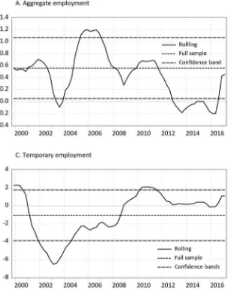
Figure 2 presents graphs of the estimated rolling coefficients, as well as the same coefficients calculated for the full sample and the 95% confidence bands for full sample estimates. The estimated parameters from rolling regression for some periods are outside confidence bands for full sample estimates suggesting the existence of a structural break. The graph of the rolling regression estimates can be interpreted as the pattern of changes of employment elasticity.
As we can observe inFigure 2, estimated parameters are indeed unstable. What is interesting, the aggregate employment elasticity exhibits a tendency to fall, and similarly pattern can be observed for permanent employment. Contrary to the expectation, the rolling coefficients started to decline around 2007, despite the large share of temporary contracts which should increase according to the theory of elasticity of employment. However, the downward trend fluctuates. Declines in the responsiveness coincided with growth slowdowns in Poland during the Great Recession (2008–2009) and in the years of 2012–2013.
This pattern is consistent with the studies which provide evidence on the instability of the Okun’s coefficient. On the other hand, it contrasts with the above-cited papers which analyse the influence of the share of term contracts on employment volatility. This inconsistency raises the question of what accounts for the decline of total employment elasticity? One way of answering
94 Acta Oeconomica70 (2020) 1, 83-104
this question is to look at the evolution of output elasticity of temporary and permanent employment. Elasticities exhibit the opposite movements. These opposite movements appear to have the potential to explain this tendency. Increasing elasticity of temporary employment has a positive effect on aggregate elasticity. In contrast, decreasing elasticity of permanent employ- ment has a negative effect on aggregate elasticity. Due to the predominant share of permanent workers, the second effect outweighed thefirst one and the total employment elasticity declined.
The temporary employment elasticity shows an upward trend. The coefficients of rolling regression are smaller than the full sample coefficients before 2008 but higher than the full sample ones starting from 2008. Particularly, a huge fall in elasticity of this type of employment was observable between 2000 and 2003. From 2003, elasticity started growing and the trend continued until 2012–2013. Then we observe a period of stabilisation. Conversely, elasticity of permanent employment tends to decrease. The estimated parameters are generally above the full sample ones before 2008, and then we can observe a decreasing tendency until 2012–2013. Next, the growth elasticity of permanent employment stabilises.
Following the discussion in Section 2, the diverging trends could not be explained by the changes in strictness of employment protection. The difference in the evolutions of temporary and permanent employment elasticity can be construed as a change in afirm’s employment strategy influenced by changing labour market conditions. It seems plausible that at the turn of the century, when unemployment became high and persistent, firms were converting open-ended contracts intofixed-term contracts in order to reduce costs.
When unemployment decreased, firms started using fixed-term contracts as the main workforce adjustment device in response to outputfluctuations. In turn, stabilization of elasticities coincided with a period of labour market tightness, when employers had dif- ficulties in finding workers due to decreasing population in working age.
Figure 2.Rolling coefficients of Eq. (1) Sources: LFS, CSO and own calculation.
The other way in which we model the instability of the parameters is by means of the Markov switching (MS) regression. Here, we assume that two states are present in the data, both of them given by model (1), but with different parameters. The probability of remaining in the same state is given by probabilities p11,p22 and the probabilities of changing the state –with probabilitiesp12,p21.
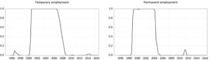
The estimated parameters of the MS regressions are obtained for separate univariate models for the permanent and temporary employment. The results of the Expectation-Maximisation (EM) procedure are reported in Table C1.Using Bayes theorem and the estimates of the pa- rameters, we obtain the ex-ante probabilities of the states (smoothed probabilities) which are represented byFigure C1.
It is noteworthy that close to one probabilities of state 1 in the model for permanent employment coincide with the close to one probabilities of state 1 in the model for temporary employment. This result suggests that the data consists of observations coming from two re- gimes. One, which was present in the years of 1996–2000 and 2005–2016, was characterised by relatively lower growth elasticity of permanent employment to changes in GDP growth and with of temporary employment which were not related to permanent employment changes. The second state (years 2000–2005) features higher sensitivity of permanent employment to changes in growth rates, but a strong negative relationship between the changes of permanent employment and temporary employment (substitution effect). What this analysis suggests is that the pre-accession period was unusual for the Polish labour market.
5. CONCLUSIONS
Our research analysed how the observed increase in use of temporary contracts affected output elasticity of employment in Poland. Our study confirms the positive output aggregate employment responsiveness, and finds that this responsiveness changes over time. Surprisingly, aggregate output employment elasticity was falling over the period of the widespread use of term contracts. The cause is the opposite trends in elasticity of permanent and temporary jobs. While the elasticity of permanent employment decreased, the elasticity of temporary employment increased. It seems that the spreading of term contracts changes the way in which labour de- mand is adjusting to output fluctuations. At the turn of century, employers used temporary workers in order to replace permanent workers and in the following years temporary workers became a workforce adjustment buffer.
Our analysis implies the following policy indications regarding to the Polish economy.
Aggregate demand policy which promotes GDP growth increases the employment growth (and decreases unemployment rate), but quantitative effects of this policy are uncertain due to instability of the Okun’s coefficient. For the same reason, predictions based on Okun’s law are also prone to large error. Spreading of temporary jobs affects to a much greater extent the employment composition than employment growth, and can be ineffective tool to cut un- employment. We believe that prevalence of unstable temporary contracts is more beneficial for employers than for employees, and that policymakers should have this imbalance in mind.
96 Acta Oeconomica70 (2020) 1, 83-104
ACKNOWLEDGEMENTS
The authors wish to thank anonymous referees for valuable comments and suggestions. We are also grateful to TomaszŁyziak and the participants of the seminar at the Institute of Economics of the Polish Academy of Sciences for their comments on the previous version of this article.
REFERENCES
Arak, P.–Lewandowski, P.–Zakowiecki, P. (2014): Fikcja zatrudnienia w Polsce_ –propozycje wyjscia z impasu (Dual Labour Market in Poland – Proposals for Overcoming the Deadlock). IBS Working Paper,No. 01/2014.
Ball, L.–Leigh, D.–Loungani, P. (2012):Okun’s Law: Fit at 50?Paper presented at the 13th Jacques Polak Annual Research Conference hosted by the IMF, Washington, D.C., November 8–9, 2012.
Bartosik, K.–Mycielski, J. (2017): The Output Employment Elasticity and the Increased Use of Temporary Contracts:
Evidence from Poland.Working PaperNo. 23/2017 (252), Faculty of Economic Sciences, University of Warsaw.
Beaton, K. (2010):Time Variation in Okun’s Law: Canada and U.S. Comparison.Bank of Canada Working Paper, No. 2010-7.
Benito, A.–Hernando, I. (2008): Labour Demand, Flexible Contracts and Financial Factors: Firm-Level Evidence from Spain.Oxford Bulletin of Economics and Statistics, 70(3): 283–301.
Bentolila, S.–Bertola, G. (1990): How Bad is Eurosclerosis?.Review of Economic Studies, 57(3): 381–402.
Bentolila, S.–Cahuc, P.–Dolado, J. J.–Barbanchon, T. (2012): Two-Tier Labor Markets in the Great Recession: France vs. Spain.The Economic Journal, 122(562): F155–F187.
Bentolila, S.– Saint-Paul, G. (1992): The Macroeconomic Impact of Flexible Labor Contracts, with an Application to Spain.European Economic Review, 36(5): 1013–1047.
Boeri, T. (2011): Institutional Reforms and Dualism in European Labor Market. In: Ashenfelter, O.–Card, D. (eds):Handbook of Labor Economics. Great Britain, North Holland, pp. 1173–1236.
Boeri, T.–Garibaldi, P. (2007): Two-Tier Reforms of Employment Protection: A Honeymoon Effect?The Economic Journal, 117(521): 357–385.
Burda, M.–Hunt, J. (2011): What Explains the German Labor Market Miracle in the Great Recession?
Brookings Papers on Economic Activity, Spring, 273–235.
Cahuc, P.–Charlot, O.–Malherbet, F. (2016): Explaining the Spread of Temporary Jobs and its Impact on Labor Turnover.International Economic Review, 57(2): 533–572.
Cazes, S.–Verick, S.–Hussami, F. A. (2013): Why Did Unemployment Respond so Differently to the Global Financial Crisis across Countries? Insights from Okun’s Law.IZA Journal of Labor Policy, 2(10): 2–18.
Central Statistical Office (2016):Employment in National Economy in 2015. Warsaw.
Central Statistical Office:Quarterly Information on the Labour Market. Warsaw, various years.
Central Statistical Office:Statistical Bulletins. Warsaw, various years.
Cichocki, S.–Gradzewicz, M.–Tyrowicz, J. (2015): Wra_zliwosc zatrudnienia na zmiany PKB w Polsce a elastycznosc instytucji rynku pracy (The Responsiveness of Employment to Changes in GDP and the Flexibility of Labor Market Institutions in Poland).Gospodarka Narodowa, 278(4): 96–116.
Ci_zkowicz, P.–Rzonca, A. (2003): Uwagi do artykułu Eugeniusza Kwiatkowskiego, Leszka Kucharskiego i Tomasza Tokarskiego, pt. Bezrobocie i zatrudnienie a PKB w Polsce w latach 1993–2001 (Comments
on the article by Eugeniusz Kwiatkowski, Leszek Kucharski and Tomasz Tokarski, titled Unemploy- ment, Employment and GDP in Poland in 1993–2001).Ekonomista, 5: 675–699.
Czy_zewski, A. B. (2002): Wzrost gospodarczy a popyt na prace¸ (Economic Growth and Labour Demand).
Bank i Kredyt, 33(11–12): 123–133.
Costain, J.–Jimeno, J. F.–Thomas, C. (2010):Employment Fluctuations in a Dual Labor Market. Banco de Espa~na Documentos de Trabajo, No. 1013.
Daly, M.–Hobijn, B. (2010):Okun’s Law and the Unemployment Surprise of 2009. FRBSF Economic Letter, March 8.
d’Agostino, G.–Pieroni, L.–Scarlato, M. (2018): Evaluating the Effects of Labour Market Reforms on Job Flows: The Italian Case.Economic Modelling, 68: 178–189.
Dixon, R. –Lim, G. C. –van Ours, J. C. (2016). Revisiting the Okun relationship.Applied Economics, 49(28): 2749–2765.
Gatti, R.–Goraus, K.–Morgandi, M. (2014):Balancing Flexibility and Worker Protection. Understanding Labor Market Duality in Poland. The World Bank, Washington, D.C.
Granger, C. W. J.–Newbold, P. (1974): Spurious Regressions in Econometrics.Journal of Econometrics, 2(2): 111–120.
G€uell, M. (2003): Fixed-term Contracts and Unemployment: An Efficiency Wage Analysis. Barcelona Economics Working Paper Series, No. 18.
IMF (2010):Unemployment Dynamic during Recessions and Recoveries: Okun’s Law and Beyond. World Economic Outlook: Rebalancing Growth, April, Chapter 3.
Jimenez-Rodriguez, R.–Russo, G. (2012): Aggregate Employment Dynamics and Partial Labour Market Reforms.Bulletin of Economic Research, 64(3): 430–448.
Hsiao, C.–Wang, S. (2007): Lag-Augmented Two- and Three-Stage Least Squares Estimators for Inte- grated Structural Dynamic Models.Econometrics Journal, 10(1): 49–81.
Kahn, L. M. (2010): Employment Protection Reforms, Employment and the Incidence of Temporary Jobs in Europe: 1995–2001.Labour Economics, 17: 1–15.
Knotek, E. S. (2007):How Useful is Okun’s Law? Federal Reserve Bank of Kansas City Economic Review, Fourth quarter: 73–103.
Lewandowski, P. (2018):Case Study–Gaps in Access to Social Protection for People Working Under Civil Law. European Commission, Brussels.
Lewandowski, P.–Magda, I. (2017): Temporary Employment, Unemployment and Employment Protec- tion Legislation in Poland. In: Piasna, A.–Myant, M. (eds):Myths of Employment Deregulation: How it Neither Creates Jobs nor Reduces Labour Market Segmentation.ETUI, Brussels, pp. 143–163.
MRPiPS (2016):Informacja o działalnosci agencji zatrudnienia w 2015 roku (Information on the Activities of Employment Agencies in 2015). Warsaw.
OECD (2004):Employment Outlook.Paris.
Okun, A. M. (1962):Potential GNP: Its Measurement and Significance. Reprinted as Cowles Foundation Paper 190.http://cowles.econ.yale.edu/P/cp/p01b/p0190.pdf.
Ryczkowski, M.–Maksim, M. (2018): Low Wages–Coincidence or a Result? Evidence from Poland.Acta Oeconomica, 68(4): 549–572.
Saczuk, K. (2014): Badanie Aktywnosci Ekonomicznej Ludnosci w Polsce w latach 1995–2010. Korekta danych (Labor Force Survey in Poland in 1995-2010. Data correction). Materiały i Studia NBP. NBP, Warsaw, No. 301.
Saget, C. (2000): Can the Level of Employment be Explained by GDP Growth in Transition Countries?
(Theory versus the Quality of Data).Labour, 14(4): 623–644.
98 Acta Oeconomica70 (2020) 1, 83-104
Social Diagnosis 2015.Objective and subjective quality of life in Poland.Rada Monitoringu Społecznego, Warsaw.
Statistical Yearbook of Social Insurance, SII–various years.
APPENDIX A. LABOUR MARKET PERFORMANCE IN POLAND – BASIC TRENDS
Figure A1.Unemployment rate (%), 1995–2016.
Note: Quarterly data, seasonally adjusted.
Source: LFS.
Figure A2.Aggregate employment and GDP growth (%), 1996–2016.
Note: Quarterly data, seasonally adjusted.
Sources: LFS, CSO and own calculation.
APPENDIX B. HEGY TEST, FM-OLS AND GRANGER CAUSALITY TEST
Table B1.HEGY tests for seasonal unit roots Employment
ΔGDP Critical value 5%
Total Permanent Temporary
t(0) 2.942 2.592 2.206 3.304 2.441
t(Pi) 7.106 6.915 6.229 6.907 2.442
F(Pi/2) 23.917 35.177 36.274 23.443 4.032
F(All_seas) 138.873 125.959 55.386 89.013 3.865
F(All) 107.019 96.044 42.848 70.153 3.723
Sources:LFS, CSO and own calculation.
Table B2.FM-OLS estimates of Eq. (1)
ΔEmployment
Total Permanent Temporary (1) Temporary (2)
ΔGDP 0.739*** 0.735 6.229 0.633
(0.285) (0.518) (1.540) (0.862)
ΔPerm. employment 2.368***
(0.471)
Constant 0.017 0.028 0.109 0.048
(0.012) (0.023) (0.067) (0.037)
N 83 83 83 83
R2 0.120 0.215 0.053 0.361
RMSE 0.026 0.034 0.182 0.111
Sources:LFS, CSO and own calculation.
Table B3.Granger causality tests
chi2 df P-value
ΔPermanent employment
ΔTemporary employment 0.927 2 0.629
ΔGDP 5.246 2 0.073
ALL 6.599 4 0.159
(continued)
100 Acta Oeconomica70 (2020) 1, 83-104
APPENDIX C. MARKOV SWITCHING REGRESSION
Table B3.Continued
chi2 df P-value
ΔTemporary employment
ΔPermanent employment 7.240 2 0.027
ΔGDP 1.121 2 0.571
ALL 10.009 4 0.040
ΔGDP
ΔPermanent employment 1.474 2 0.479
ΔTemporary employment 0.509 2 0.775
ΔGDP: ALL 1.537 4 0.820
Sources:LFS, CSO and own calculation.
Table C1.Estimates of parameters of Markov switching model
Employment
Permanent Temporary
State 2
ΔGDP 0.708*** 0.086
(0.214) (0.850)
ΔPermanent employment 1.936***
(0.435)
Constant 0.070*** 0.145***
(0.009) (0.043)
State 1
ΔGDP 0.342*** 0.343
(0.130) (0.373)
ΔPermanent employment 0.284
(0.264)
Constant 0.004 0.008
(0.006) (0.016)
(continued)
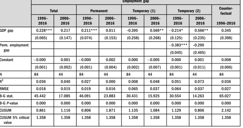
APPENDIX D. ESTIMATION OF THE “ GAP ” EQUATION
To check the sensitivity of our analysis we conduct the same exercises with“gap”Eq. (2) as the
“difference”Eq. (1). In order to estimate the trend component, we follow the standard practice of using the Hodrick-Prescott (HP)filter withλcoefficient equal to 1600. Additional equation in which temporary employment is explained not only by GDP growth but also by permanent employment growth takes the form:
ΔeTt ΔeT*t
¼b0þb1 ΔytΔy*t
þ ΔePt ΔeP*t
þ«t (5) whereeTand ePare temporary and permanent employment respectively. Table D1 shows the static Okun’s coefficients, Figure D1 presents the rolling regressions. The results are, to a large extent, consistent with the “difference” specification presented above. For instance, rolling regression confirms downward trend of output aggregate employment elasticity, and opposite trends elasticities of permanent and temporary employment.
Table C1. Continued
Employment
Permanent Temporary
Sigma 0.019 0.047
(0.002) (0.004)
p11 0.941 0.952
(0.050) (0.041)
p21 0.016 0.017
(0.016) (0.019)
N 84 84
Note:Standard error in parentheses. Wald statistic cannot be used for testing the significance of sigma, p11, p21 and then stars for these parameters were omitted.
Sources:LFS, CSO and own calculation.
Fig. C1.Probability of state 1.
102 Acta Oeconomica70 (2020) 1, 83-104
Table D1.OLS estimations Eq. (2)
Employment gap
Total Permanent Temporary (1) Temporary (2) Counter-
factual 1996–
2016 2006–
2016 1996–
2016 2006–
2016 1996–
2016 2006–
2016 1996–
2016 2006–
2016 1996–2016
GDP gap 0.228*** 0.217 0.211*** 0.011 –0.395 0.569** 0.214* 0.566** 0.345
(0.065) (0.147) (0.074) (0.153) (0.258) (0.268) (0.125) (0.235) (0.398)
Perm. employment gap
0.383*** –0.290 (0.045) (0.465)
Constant 0.000 0.001 0.000 0.002 0.000 0.005 0.000 0.001 0.008
(0.001) (0.002) (0.001) (0.004) (0.002) (0.007) (0.001) (0.011) (0.006)
N 84 44 84 44 84 44 84 44 84
R2 0.036 0.040 0.027 0.000 0.008 0.048 0.051 0.073 0.036
RMSE 0.018 0.015 0.019 0.016 0.065 0.037 0.064 0.037 0.027
B-G stat. 45.442 17.085 46.091 23.883 30.431 15.925 30.554 14.263 65.027
B-GP-value 0.000 0.000 0.000 0.000 0.000 0.000 0.000 0.000 0.000
CUSUM 0.861 1.116 0.806 1.871 1.135 1.084 1.129 0.806 2.142
CUSUM 5% critical value
1.358 1.358 1.358 1.358 1.358 1.358 1.358 1.358 1.358
Notes:B-G: Breusch-Godfrey autocorrelation test, Newey-West standard errors in parentheses,/***/**/*/indicate statistical significance at the 1, 5, and 10 per cent level, respectively.
Sources:LFS, CSO and own calculation.
mica70(2020)1,83-104103
Fig. D1.Rolling regression of the“gap”equation.
Sources: LFS, CSO and own calculation.
104 Acta Oeconomica70 (2020) 1, 83-104