Figure 1. Manually annotated tissue image
Evaluation and Comparison of Cell Nuclei Detection Algorithms
Sándor Szénási*, Zoltán Vámossy**, Miklós Kozlovszky***
* Óbuda University, Doctoral School of Applied Informatics, Budapest, Hungary
** Óbuda University, John von Neumann Faculty of Informatics, Budapest, Hungary
*** MTA SZTAKI, Laboratory of Parallel and Distributed Computing, Budapest, Hungary szenasi.sandor@nik.uni-obuda.hu; vamossy.zoltan@nik.uni-obuda.hu; m.kozlovszky@sztaki.hu
Abstract— The processing of microscopic tissue images and especially the detection of cell nuclei is nowadays done more and more using digital imagery and special immunodiagnostic software products. Since several methods (and applications) were developed for the same purpose, it is important to have a measuring number to determine which one is more efficient than the others. The purpose of the article is to develop a generally usable measurement number that is based on the “gold standard” tests used in the field of medicine and that can be used to perform an evaluation using any of image segmentation algorithms. Since interpreting the results themselves can be a pretty time consuming task, the article also contains a recommendation for the efficient implementation and a simple example to compare three algorithms used for cell nuclei detection.
Keywords: biomedical image processing, nuclei detection, region growing, K-means
I. EVALUATION METHODS OF TISSUE SAMPLE SEGMENTATION ALGORITHMS
Image segmentation is one of the most critical tasks of computer vision. Its main purpose is to split the input image into parts, and then the identification of those parts.
There are several methods to analyze tissue samples; we can find numerous publications about new methods even if we only look for a specific sub-topic, for example cell nuclei detection in colon tissues: [1][2][3][4][5]
[6][7][8][9]. It is very hard to compare these methods, because they try to get the same results through very different approaches, but we still need some kind measurement numbers that can be easily interpreted and that can provide us with a consistent, easy-to-handle value. This is especially important if the aim of the research is the improvement of an already existing method or the development of a new method based on an old one, because the true verification of the experimental results is only possible if such a number exists. The goodness of an algorithm can be interpreted from several points of view, in our task the important factors are the accuracy and the execution time. In addition to that, it would be practical to find a goodness function that can be easily handled and that can be quickly evaluated so that it can be used for automatic parameter optimization too.
Naturally, there are several available methods to evaluate the accuracy of different algorithms; according to their analytical approach these can be separated into the following groups [10]:
Simple analytical: these analytical methods directly examine the segmentation algorithm itself (basic principles, pre-requirements,
complexity, etc). In practice, this approach can only be used efficiently in some special cases, because there are no generally usable, comprehensive theoretical models in the field of image processing.
Empirical goodness: the empirical methods are always based on the execution of the examined algorithms on some test images, and then the evaluation of the algorithms’ output for these images. The empirical goodness methods try to analyze only the results themselves, according to some goodness factors based on some human intuitions.
Empirical discrepancy: these methods also examine the output of the algorithms for some test images, but the main difference is that in this case a reference result set is also present (with the correct expected results), so the base of the goodness calculation is the comparison of the expected and the actual results. It is also beneficial because it seems easier to assign a number for the similarity to the correct results than to assign a number for some absolute degree of goodness.
Since the algorithms that will be analyzed will mainly identify objects that can be found in tissue samples, it is feasible to take into account the methods of medical examinations as well. In the practice of the clinical work, it is fairly common to do evaluation based on the “gold standard” tests [11], which are similar to the “empirical discrepancy” group from the list above. For this, we need some test images with a reference result set (gold
standard): this usually means images annotated by a skilled pathologist (or in the ideal case: the merged results of images annotated by several skilled pathologists).
The most general solution is based on the confusion matrix [12] that can be constructed using comparing the two result sets. The matrix (assuming we have two possible outcomes) contains the number of true positive, true negative, false negative and false positive hits. This classification is very often used in medical examinations, and we can also very simply and very efficiently use it to evaluate image processing algorithms, where:
true positive (TP): the pixel is correctly classified as part of a cell’s nucleus in both the reference result set and in the test result set as well;
true negative (TN): the pixel is correctly classified as not part of a cell’s nucleus in both the reference result set and in the test result set as well;
false positive (FP): the pixel is not classified as part of a cell’s nucleus in the reference result set, but in the test result set the pixel is mistakenly classified as part of a cell’s nucleus;
false negative (FN): the pixel is classified as a part of a cell’s nucleus in the reference result set, but in the test result set the pixel is mistakenly not classified as a part of a cell’s nucleus.
In the list above, “reference result set” means the images annotated by the doctors, and “test result set”
means the output of the evaluated algorithm. The measurement number can be interpreted for the whole examined image, but also in pairs to compare specific pixel groups. Since at the moment we only want to locate cell nuclei, we do not need to establish more classes.
After this, the accuracy of the algorithm is a simply calculated measurement number (the ratio of the positive classifications in the complete set) [12]:
Accuracy = (TP + TN) / (TP + TN + FP + FN)
In addition to this, we often need the values for precision and recall [12]:
Precision = TP / (TP + FP) Recall = TP / (TP + FN)
These values are very expressive (e.g. a 100% of accuracy means that the algorithm gives exactly the same results as the reference result set, and 0% means that none of the pixels were correctly classified). In addition to this, these percentage values are not required to be separately normalized.
It is possible to find several other methods that can be used to further refine these numbers. For example, we could take into account the minimum distance between a wrongly classified pixel and the nearest pixel that actually belongs to the class we wrongly classified the given pixel into [10].
However, the pixel-level evaluation itself will not give us a generally acceptable result, because during the segmentation our task is not only to determine if a pixel belongs to any object or not, but we have to locate the objects themselves. Because of this, it is often practical to examine the number of detected objects, and check how big the difference is between the reference results and the results of our examined algorithm. It is also practical to further refine this experiment by going further than merely
counting the objects: we should measure the different geometrical parameters of the detected objects as well. In case of the cell nuclei we want to examine, these geometrical parameters are: centre of mass, diameter, and the location of every pixel [13].
For the final evaluation, the pixel-level and the object- level comparisons can be both necessary. Naturally the two methods are not exclusive, what is more, it would be practical to use a goodness function that incorporates them both [14], for example we can calculate the results separately for every different aspects, and then sum up the results using proper weighting and normalization. This solution can later be very effective, because this way we can take into account some significantly different aspects as well, for example the execution time of the processing program, which is not shown in these results, but it still greatly affects the practical usability of the given method.
Finding the proper weights and ratios is of course a considerably difficult problem, but hopefully this method will be suitable to compare the different algorithms even in this case.
II. CREATING A SELF-MADE MEASUREMENT NUMBER A. Accuracy
The easiest method that simply compares the test result set with a reference set using a pixel-by-pixel comparison is not good enough when processing images of tissue samples, because it will only show a small error even for big changes in densities (for example in the case of many false negative detection for many small cell nuclei objects). Because of this it is practical to process the cell nuclei themselves as separate objects, but even in this case the usage of some statistical features (e.g. number of objects, density) and the usage of some geometrical data (location, size) are not enough, because the shapes of the cell nuclei can also be important for the diagnosis.
Because of these, our measurement number does not only reflect a pixel-by-pixel comparison; instead it starts by matching the cell nuclei together in the reference results and in the test results. One cell nucleus from the reference result set can only have one matching cell nucleus in the test result set, and this is true the other way around too: one cell nucleus from the test result set can only have one matching cell nucleus in the reference result set. This is a considerably strict rule, but because of this rule the evaluation of the results is a lot easier, because we do not need corrections due to areas that have multiple matches.
After the matching of the cell nuclei, the next step is the similarity comparison between the paired elements. Since the further processing steps might require the exact shape and location of the cell nuclei, it is not worthwhile to compare the derived parameters of the individual cell nuclei (e.g. it is not worthwhile to calculate the area, circumference, diameter, etc. for all cell nuclei and then compare these properties), instead it is more practical to choose a pixel-by-pixel comparison. Because of this, after pairing up the cell nuclei we try to evaluate the test result using a comparison like this one.
The pixel-by-pixel comparison is a long-time existing and well working technique, its output is usually a quartet of integers that represent the number of true positive, true negative, false positive, and false negative hits, respectively. The interpretation of the true positive hits is
simple: every correlating pixel is calculated using the same weight. The number of true negative hits can only be calculated for the whole image, or (when using “gold standard” images) for the manually annotated parts of the images; this value will essentially be the number of pixels that are classified as not part of a cell nuclei both in the reference result set and in the test result set as well.
With the false positive and false negative hits, we can work with the already existing terminology, but here it is not practical to use the same equal weights as with the true positive and true negative hits, but instead it is better to take into account the distance between the wrongly classified pixel and the contour of the cell as well. The reason for this is that it is usually very hard to clearly determine the contour of the cell nuclei (for example it can mean a great difference whether the inner or the outer contour was marked on the test and the reference images).
Because of this, errors near the contour must have a lower weight than the errors that are far away from it. Since the maximum tolerated distance greatly depends on the resolution and on the zoom factor, it is practical to determine this threshold as a ratio of the reference (biggest) cell nucleus’ diameter:
Weighti = Min(Minj(Dist(Ti , Rj)) / Diameter(R)*KT), 1)
Dist(Ti , Rj) – distance between the tested cell nucleus’ ith pixel and the reference cell nucleus’
jth pixel;
Diameter(R) – diameter of the reference cell’s nucleus;
KT – constant parameter.
In this expression KT is a constant that helps us in setting a distance limit (relative to the reference cell nucleus’ diameter): over this limit an erroneous pixel detection is considered to be an error with the weight of 1 (for example with KT = 0.5 a distance greater than half of the diameter is over this limit). For distances lower than this limit, we calculate the weight to be linearly proportional with the distance. By setting the value of this constant, we can also determine how strictly we want to take the differences into account (for example with KT = 0 all false positive pixels are counted with the weight of 1).
The same method can be used for the false positive and for the false negative hits as well, where the end result will not only show the number of pixels, but the weighted value that is calculated as it is described above.
If there is a cell nucleus in the reference image to which we could not find a matching cell nucleus in the test result set (or vice versa), then the pixels of that cell nucleus can be considered (with the weight of 1) as false positive of false negative pixels. By summing up the values calculated for the cell nucleus pairs (or for the individual cell nuclei), we can calculate a simple accuracy value (assuming that the reference result set contained at least one cell nucleus): (TP + TN) / (TP + TN + FP + FN). The end result will be exactly 1 if the algorithm found exactly as much cell nuclei as there was in the reference result set, and furthermore the pixels of the individual cell nuclei are pair wise the same. In case of missing or erroneous hits this value decreases, and it becomes 0 if no correct pixels were found.
B. Execution time by image resolution
The different methods that try to evaluate the goodness of a segmentation algorithm usually do not consider the
execution time. This can be understood in cases where the image processing is not time critical, or when the whole process takes such a short time that the user will not even notice the differences. However, this can be an important factor in the case of real-time applications or with algorithms where the execution time is very long – both is true when processing images of microscopic tissue samples. Since we have to process large images [15] in real time, even if we have an algorithm with very good accuracy, the execution time using an average zoom level could prevent us from using them in a real-world example.
For example, the execution time for an implementation of the region growing cell nucleus search algorithm (that will be described later in this paper) can be as long as one hour when we process a large image (with a resolution of 8192×8192). In this scale, even if we can reach a four or five times faster execution time, it greatly improves the practical usability of the method.
When measuring the execution time, we do not measure the time for the required operations to start the program by the operating system. The same way we ignore the time required to load the input or store the output. The steps between these two are considered as one unit, since these belong to the search process, and these parts are not separable: preprocessing (creating copies of the images, executing various filters), performing the search (the actual cell nuclei detection process), post-processing (classification of the found cell nuclei, post-filtering, perhaps some further processing).
The measurements described above greatly depend on the hardware environment [16] that is used when performing the experiments, but since the aim is to compare the disposable algorithms, executing them using the same hardware allows us to ignore this (hardly measurable and hardly expressed) parameter.
Regarding the description above, our time measurement method is the following:
1. Launch the application.
2. Execute the algorithm for the first time without measuring the elapsed time (warm-up). This first execution is not used for the measurements, because various compiling operations can still occur here, and the caches are not filled up either, unlike at the later executions.
3. Execute N consecutive runs with the algorithm, note up the execution times.
4. Calculate the average execution time using the previous measurements.
The execution time greatly depends on the size of the image, so it is practical to normalize the results. This could be a simple division with the number of pixels on the image, but this approach can produce data that can be hard to compare, because only a relatively small part of the big image contains the tissue sample itself, and quite often only a fraction of the sample shows the cell nuclei themselves. For this reason, this number showed too large deviation in the practical tests: when timing the same algorithm it displayed a lot bigger speed for a large image with just a few cell nuclei while it displayed a slower speed for a small image with lots of cell nuclei. Because of this, for normalization purposes, it is more practical to consider the number and size of the cell nuclei, since we already know the output of the accuracy tests. Due to
these reasons, using this measurement number with the latter normalization method is far more useful:
Processing Speed = Execution Time / TP Pixel Count This way this measurement number actually tells us that in average how long it took for the algorithm to find a cell nuclei pixel. This is a fairly strict evaluation method, because the execution time contains the examination of false positives and areas not belonging to any cells, but since the former is not considered as “valuable” work, and the latter was already ignored when measuring the accuracy, this value seems to be the most effective measurement number to compare different algorithms.
The resulting measurement number is naturally different for every different image (depending on the properties of the image), so using this method we can only compare algorithms that work on the same input images.
It is advised to execute this comparison for every type of tissue samples that can typically occur in a real world scenario (healthy sample, diseased sample, erroneous sample, etc), but this can easily be achieved by using the aforementioned “gold standard” tests, because this way there is a collection at hand with 40 included samples that contain tissue samples of different properties.
III. IMPLEMENTING A COMPARISON ALGORITHM The accuracy evaluation method described above performs a reasonably precise object and pixel-based comparison, while it considers the unique features of cell nuclei detection. The very critical point of the evaluation is that how the cell nuclei are matched against each other in the reference and the test result sets, because obviously this greatly affects the final result. Since this pairing can be done in several ways (due to the overlapping cell nuclei) it is important that from the several possible pair combinations we have to use the optimal: the one that gets the highest final points.
Implementing the evaluation method described above becomes harder because it has fairly high computational needs: there are several thousand cell nuclei in a bigger image, and finding the optimal pairing combination from all the possible combinations using a simple linear search would end up in an execution time that is unsuitable for any practical use. Naturally we do not need to try the pairing of two cell nuclei that are far away from each other, so the number of combinations that we have to examine is a lot lower, but still, determining which cell nucleus should be paired with which other cell nucleus cannot always be determined in one step, especially when
we have several objects that are close to each other.
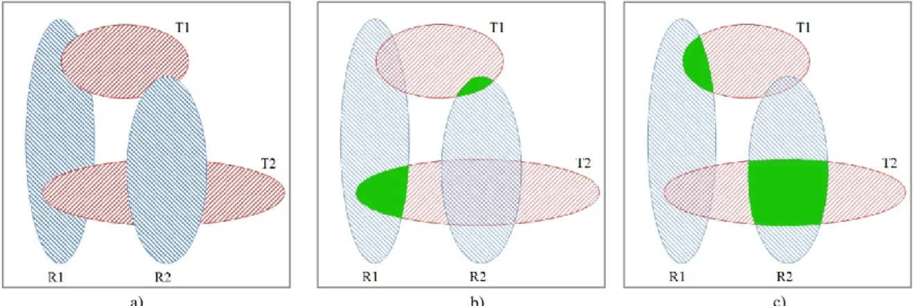
A typical example can be seen in Figure 2. If we try to find pairs using a greedy algorithm, then processing the R1 reference cell nucleus is the first step. We should pair it up with cell nucleus T2 (because the number of overlapping pixels is the biggest). As a result, the next reference cell nucleus (R2) can only be paired up with cell nucleus T1, and it is clearly visible that this is not an optimal solution: if we reverse the pairs, then the total number of overlapping pixels is greater. This example shows that we cannot simply choose the solution that looks the best at the moment (in the order of processing), but in case of overlapping cells we have to consider the other possible choices too. In the example above this means the analysis of 2 cases (which becomes 7 distinct cases if we allow unpaired cell nuclei as well), but naturally the number of possible combinations can be even bigger if there is a fifth cell nucleus that overlaps one or more of the others (in the practical application, long chains of overlapping cells are formed with as much as 50 cell nuclei in the chain).
The detected cell nuclei can usually be evaluated independently; there is no need to compare every single cell nucleus with every other one. It is usually practical to create groups from the cells that require further processing to find the pairs amongst them. This can be done using a method similar to the clustering algorithms [17]: we take an arbitrary cell nucleus from the reference set, and we consider it as the first element of its group. After this, we take the cells from the test set that overlap with this one, and we add them to the same group. After this, we loop through the reference set again, and we add the cells into the group that overlap any of the test cells from the group.
We continue this iteration of switching between the test and reference sets until the group is no longer extended. In the end, the group will contain the biggest possible set of those elements where it is possible to reach any element from any element with a limited number of steps through a chain of overlapped cells.
It is possible (both in the reference set and in the test set as well) that there will be some cell nuclei that do not overlap with other cells; these will create a group on their own. If we perform this grouping for all cell nuclei, then we will get some distinct and easily manageable groups where every cell nucleus is a member of exactly one group, and where there is absolutely no overlap between two cells of different groups. Due to this, the paring of the cell nuclei can be done within the group, and this greatly
Figure 2. (a) Blue reference cells: R1, R2; red test cells: T1, T2 (b) First pairing: R1-T2, R2-T1 (c) Second pairing: R1-T1, R2-T2
a) b) c)
reduces the computational needs of the calculation.
During the practical analysis of the results we found out that on areas where cells are located very densely, we have to loop through a very long chain of overlapped cells, which results in groups that contain very much cell nuclei from the test and from the reference sets as well.
Since increasing the number of elements in a group exponentially increases the processing time of the group, it is practical to find some efficient algorithm for the matching: we use a modified backtracking search algorithm [18].
The sub-problem of the backtracking search is finding one of the overlapping cell nuclei from the test results and assigning it to one of the reference cell nuclei. For this, we have to collect the reference cell nuclei from the group, and assign an array to each of them. Then we have to fill the array for every reference cell with test cells from the group that overlap with the given reference cell (PTCL- Potential Test Cell in this Level), because we only have to perform the search for the elements of this array. Due to the special nature of the task, we do not expect to solve all sub-problems, so it is possible that there will be some reference cells with no test cell nucleus assigned to them.
For the same reasons, it is also possible that there will be some test cells with no assignment at all.
The final result of the search is the optimal pairing of all the possible solutions (we want the solution where (using the evaluation described above) we can achieve the biggest possible pixel-level accuracy within a group). The number of possibilities that have to be examined is still pretty high, but we can reduce this even more using an additional backtrack condition: for every reference cell nucleus we calculate and store a value (LO) that represents the local optimal result, if we always choose the best overlapping test cell that seems optimal at the moment.
During the search, the algorithm will not move to the next level if it is found out that the calculated value will always be worse than this LO value even if we choose the most optimal choices on all the following levels.
According to these, the following pairing will be performed by algorithm 1. Inputs:
level – the level currently being processed by the backtracking search;
RES – The array that holds the results.
Utilized functions:
SCORE(X) – it returns the value for the pixel- level comparison using input X (which is a pair of a test and a reference cell nuclei).
Algorithm 1 will search and return the optimal pairing of a group containing test and reference cell nuclei. The ith element of the MAXRES array shows that the ith reference cell nucleus should be paired with the MAXRES[i] test cell nucleus (or if the value is , then the reference cell should be left alone).
The algorithm above should be executed for every group, and this way the optimally paired elements can be located (including the elements that are alone in their group and the elements that cannot be paired at all). After this, we can apply the evaluation described above for every pairs (and single elements), and after summing up the values, we can determine the weighted total TP, FP, FN pixel numbers that represent the whole solution. These can be interpreted on their own (for example this might be required when setting some parameters automatically), or in a simple way (for a more spectacular comparison) using the aforementioned accuracy equation:
Accuracy = (TP + TN) / (TP + TN + FP + FN)
The accuracy could of course be calculated for the individual cell nuclei pairs as well (in this case, we should leave out the TN values from the equation), and the results we can obtain this way can be interpreted in many ways.
For example, there could be a practical use of this for determining that how many cell nuclei were successfully detected within a given class of accuracy. The measurement number described above is more practical because we do not need to individually apply weights to the individual cell nuclei, because the pixel-level results already contain weighting factors.
IV. PRACTICAL EXPERIENCES
We have implemented the above described algorithm and we have compared three cell nuclei detection algorithms. This section contains the comparison results.
Region growing was the first examined segmentation method. The basic approach is to start from a set of seed points and then appending to each one the most promising neighboring pixels that satisfy a predefined criterion based on similarities in color or intensity [19]. In some cases these growing processes can be executed in a parallel way, therefore we analyzed the single-thread implementation running on a CPU [7] and a multi-threaded implementation running on a GPU [20].
The third examined segmentation method was the K-means algorithm. This is a classical clustering method and in this case we used the segmentation of the image to find the pixels of the cell nuclei. We have used the K- means implementation prepared by the Biotech group of Try(level,RES)
for(TCPTCL[level])
if(TCRES[1..level-1]TC=) RES[level]TC
if (level=N)
if (score(RES)>score(MAXRES)) MAXRES←RES
else
if (score([RES[1..level] LO[level+1..N]])<score(MAXRES)) Try(level+1,RES)
return MAXRES
Algorithm 1. – Backtracking core algorithm
Óbuda University. After this clustering we have to split these areas to separate the independent nuclei. To achieve this, we use erosion to locate the center (or centers if we assume that the detected region consists of two or more nuclei) of the region. After we have located these centers, we must use a simplified region growing to find the actual areas of nuclei.
In practice the output of the implemented evaluator application are some numerical results (number of TP, TN, FP, FN pixels; number of excluded pixels: number of pixels outside the manually annotated area; accuracy;
processing speed) and the images that are shown in Figure 3. We can store these results in image databases for further analysis [21].
a) Original slide (cropped and scaled for this paper).
b) Gold standard result (GS) – blue line surrounds the annotated area, the red items are the manually annotated cell nuclei.
c) Region growing CPU result (RG-C) – red areas are the detected nuclei, different shades indicate different nuclei.
d) Region growing GPU result (RG-G) – red areas are the detected nuclei, different shades indicate different nuclei.
e) K-means result (KM) – red areas are the detected nuclei, different shades indicate different nuclei.
f) RG-C compared to GS. Meaning of pixel colors:
green – TP, white – TN, red – FP, blue – FN, yellow – pixel is out of the manually annotated area.
g) RG-G compared to GS (same color markings as f).
h) KM compared to GS (same color markings as f).
Figure 3. (a) Original slide (b) GS result (c) RG-C result (d) RG-G result (e) KM result (f) RG-C compared to GS (g) RG-G compared to GS (h)
KM compared to GS
a) b) c)
d) e) f)
g) h)
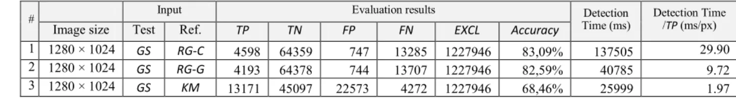
Table 1. shows the numerical results are the followings:
a) Number of TP pixels (RG-C: 4598, RG-G: 4193, KM: 13171)
b) Number of TN pixels (RG-C: 64359, RG-G:
64378, KM: 45097)
c) Number of weighted FP pixels (RG-C: 747.44, RG-G: 744.46, KM: 22573.2)
d) Number of weighted FN pixels (RG-C:
13285.35, RG-G: 13706.97, KM: 4272.0) e) Number of excluded pixels (out of the manually
annotated area, 1227946 in every cases)
f) Accuracy (RG-C: 83.09%, RG-G: 82.59%, KM:
68.46%)
g) Detection time (RG-C: 137505ms, RG-G:
40785ms, KM: 25999ms)
h) Detection time/TP (RG-C: 29.9ms/px, RG-G:
9.72ms/px, KM: 1.97ms/px) CONCLUSIONS
We have used all of these algorithms for the 40 “gold standard” slides. Our first observations:
a) The accuracies of the RG-C and RG-G implementations are almost the same. The base algorithm is identical; the small differences in the results are caused by the different processing order of the seed points.
b) The KM method is spectacularly faster than the RG implementations. Although the performance of the RG-G implementation is appropriate for practical use.
c) Mostly (except 4 cases) the accuracy of the KM method is below the accuracy of the RG methods. But considering its speed, it can be ideal for preliminary results.
d) Both of the RG-C and RG-G methods are too careful they left a lot of nuclei unprocessed. We may want to reconfigure the parameters of seed searching.
e) The KM method can find some true positive pixels in case of problematic images as well (poorly focused, difficult to interpret), but it will find several false positive pixels too, therefore the results are not as promising as it may look for the first sight.
ACKNOWLEDGMENT
The authors gratefully acknowledge the grant provided by the project TÁMOP-4.2.2/B-10/1-2010-0020, Support of the scientific training, workshops, and establish talent management system at the Óbuda University.
REFERENCES
[1] Z. Shebab, H. Keshk, M. E. Shourbagy, “A Fast Algorithm for Segmentation of Microscopic Cell Images”, ICICT '06. ITI 4th International Conference on Information & Communications Technology, 2006
[2] J. Tianzi, Y. Faguo, F. Yong, D.J. Evans, “A Parallel Genetic Algorithm for Cell Image Segmentation”, Electronic Notes in Theoretical Computer Science 46, 2001
[3] Y. Surut, P. Phukpattaranont, “Overlapping Cell Image Segmentation using Surface Splitting and Surface Merging Algorithms”, Second APSIPA Annual Summit and Conference, 2010, pp. 662–666
[4] J. Hukkanen, A. Hategan, E. Sabo, I. Tabus, “Segmentation of Cell Nuclei From Histological Images by Ellipse Fitting”, 18th European Signal Processing Conference (EUSIPCO-2010), 2010 Aug 23-27, Denmark
[5] X. Du, S. Dua, “Segmentation of Fluorescence Microscopy Cell Images Using Unsupervised Mining”, The Open Medical Informatics Journal 2010-4, 2010, pp. 41-49
[6] R. Pohle, K. D. Toennies, “Segmentation of medical images using adaptive region growing”, 2001
[7] Pannon Egyetem, “Algoritmus- és forráskódleírás a 3DHistech Kft. számára készített sejtmag-szegmentáló eljáráshoz”, 2009 [8] A. Reményi, S. Szénási, I. Bándi, Z. Vámossy, G. Valcz, P.
Bogdanov, Sz. Sergyán, M. Kozlovszky, "Parallel Biomedical Image Processing with GPGPUs in Cancer Research", LINDI 2011, Budapest, 2011 ISBN: 9781457718403, pp. 245–248 [9] L. Ficsór, V. S. Varga, A. Tagscherer. Zs. Tulassay, B. Molnár.,
"Automated classification of inflammation in colon histological sections based on digital microscopy and advanced image analysis." Cytometry, 2008, pp. 230–237.
[10] W.A.Yasnoff, J.K.Mui, J.W.Bacus, “Error measures for scene segmentation”, Pattern Recognition 9, pp. 217-231
[11] S. Timmermans, M. Berg, “The Gold Standard-The Challenge of Evidence-Based Medicine and Standardization in Health Care”, Temple University Press, Philadelphia, 2003, ISBN 1592131883 [12] R. Kohavi, F. Provost, “Glossary of Terms”, Machine Learning
vol.30 issue 2, Springer Netherlands, 1998, pp. 271-274, ISSN 08856125
[13] P. Correia, F. Pereira, “Objective Evaluation of Relative Segmentation Quality”, ICIP00, International Conference on Image Processing, 2000, vol.1, pp. 308-311
[14] M. Everingham, H. Muller, B. Thomas, “Evaluating Image Segmentation Algorithms using the Pareto Front”, Proceedings of the 7th European Conference on Computer Vision-Part IV, May 28-31, 2002, pp. 34-48
[15] Nagy, A., Vámossy, Z., „Super-resolution for Traditional and Omnidirectional Image Sequences”, Acta Polytechnica Hungarica, vol. 6/1, pp. 117–130, 2009, ISSN 1785 8860
[16] Gy. Györök, M. Makó, J. Lakner, “Combinatorics at Electronic Circuit Realization”, Acta Polytechnica Hungarica, vol. 6/1, pp.
151-160, 2009
[17] J. Han, M. Kamber, “Data Mining. Concepts and Techniques”, Elsevier Inc., 2001, ISBN 1558604898
[18] M. T. Goodrich, R. Tamassia, “Algorithm Design”, John Wiley &
Sons, Inc., 2002, ISBN 0471383651
[19] C. Smochină, “Image Processing Techniques and Segmentation Evaluation”, 2011
[20] S. Szénási, Z. Vámossy, M. Kozlovszky, “GPGPU-based data parallel region growing algorithm for cell nuclei detection”, 12th IEEE International Symposium on Computational Intelligence and Informatics (CINTI), Budapest, Nov. 2011, pp. 493 - 499, ISBN 978-1-4577-0044-6
[21] Sz. Sergyán, "A new approach of face detection-based classification of image databases", Acta Polytechnica Hungarica, vol. 6/1, pp. 175-184, 2009
# Input Evaluation results Detection
Time (ms) Detection Time /TP (ms/px) Image size Test Ref. TP TN FP FN EXCL Accuracy
1 1280 × 1024 GS RG-C 4598 64359 747 13285 1227946 83,09% 137505 29.90 2 1280 × 1024 GS RG-G 4193 64378 744 13707 1227946 82,59% 40785 9.72 3 1280 × 1024 GS KM 13171 45097 22573 4272 1227946 68,46% 25999 1.97
Table 1. Comparison results for tissue sample “B2007_00259_PR_02_validation”, KT = 0.3