Comparison and affine combination of generalized barycentric coordinates for
convex polygons
Ákos Tóth
Department of Computer Graphics and Image Processing Faculty of Informatics, University of Debrecen
toth.akos@inf.unideb.hu
Submitted April 10, 2017 — Accepted June 18, 2017
Abstract
In this paper, we study and compare different types of generalized bary- centric coordinates in detail, including Wachspress, discrete harmonic and mean value coordinates for convex,n-sided polygons. Contour lines are com- puted in each barycentric coordinate method, and curvature plots of these contour line curves are visualized. Moreover, different distortions of uniform patterns are also shown, providing exact visual method to compare these methods. To overcome the shortcomings of different generalized barycentric computations, affine combination of methods is provided.
Keywords: barycentric coordinates, Wachspress coordinates, discrete har- monic coordinates, mean value coordinates, affine combination
MSC:52B55, 52A38, 65D05
1. Introduction
Barycentric coordinates were first introduced by Möbius [1] in 1827. Any point v inside a trianglev1, v2, v3can be obtained by weighted sum of these vertices, if cor- responding weightsw1, w2, w3are placed at the vertices of triangle. These weights w1, w2, w3 are the barycentric coordinates of pointv. This can be generalized for arbitraryn-sided polygons in the plane where an inner point v can be defined as
http://ami.uni-eszterhazy.hu
185
the weighted sum of verticesv1, . . . , vn as
v= w1(v)v1+. . .+wn(v)vn
w1(v) +. . .+wn(v) .
These barycentric coordinates can be normalized that values sum to one, thus they vary linearly inside the polygon. Therefore many applications often use them to interpolate different values which are placed at the vertices of the polygon. In com- puter graphics, this interpolation is used e.g. for shading or geometry deformation.
In the last couple of years, many approaches have been released which tried to generalize the barycentric coordinates. The first generalization appeared in Wach- spress’s pioneering work [2] in 1975. The computation of Wachspress coordinates is simple for any convex polygons, because they are rational functions and their derivatives can also be easily evaluated. They have many nice properties [3] such as affine invariance or smoothness, but they are not well-defined for star-shaped polygons and for arbitrary concave polygons.
Later, new generalizations of barycentric coordinates are published, such as discrete harmonic [4] and mean value coordinates [5]. The discrete harmonic co- ordinates have the same requirements as Wachspress coordinates. They are well defined for convex polygons and they are based on the minimization of an energy function, but unlike Wachspress or mean value functions these coordinates are not necessarily positive over the interior of any convex polygon. The mean value coor- dinates are probably the most popular type of generalized barycentric coordinates.
They are well defined everywhere in the plane for any simple, star-shaped or ar- bitrary polygon. If the polygon is not star-shaped or convex, these coordinates are not necessarily positive, but in case of complex geometric shapes they are very robust. Owing to the above-mentioned properties and advantages, the general- ized barycentric coordinates are commonly used in computer graphics and image processing for parameterization of meshes [9, 10, 12], mesh deformation [7, 6, 8], transfinite interpolation [18], image warping [17], cloning [13] or symmetrization [11].
Floater et al. [14] had already provided an overall picture of barycentric coor- dinates and visualized these coordinates using the contour lines of the coordinate functions. These contour lines mean those points of the polygon where one of the barycentric coordinates is constant. In this paper, we provide a much detailed com- parison of the three different methods, we examine the Wachspress, the harmonic and the mean value coordinates and compare these functions for convex, n-sided polygons in an exact way. Moreover, to overcome the drawbacks of each method, we investigate an affine combination of these generalized barycentric coordinates.
In the next section, we give a short overview of some important definitions and properties of these barycentric coordinate methods. In Section 3, we discuss how the different coordinate functions can be comparable. Then, in Subsection 3.3, we present our results and we highlight the advantages and disadvantages of the distinct barycentric coordinates. The affine combination of the methods is described in Section 4.
2. Barycentric coordinates on n -sided polygons
Definition 2.1. LetPbe a convex polygon in the plane, with verticesv1, v2, . . . , vn
and n≥3. We call any functionsbi:P →R, i= 1. . . n,barycentric coordinates, if they satisfy the following properties for allv∈P:
bi(v)≥0, i= 1, . . . , n, Xn
i=1
bi(v) = 1, Xn
i=1
bi(v)vi=v.
2.1. Wachspress coordinates
Wachspress coordinates are the simplest and earliest generalized barycentric coor- dinate functions and they have some important properties, for example, they are affine invariant, smooth (C∞) and can be comuted by rational polynomials. These coordinate functions were published by Wachspress [2] and Warren [15], then Meyer et al. [3] simplified the formula and defined the coordinates in the following way:
bi(v) = wi(v) Pn
j=1wj(v), with
wi(v) = Ci(v) Ai−1(v)Ai(v),
whereCi(v), Ai−1(v), Ai(v)are areas of triangles shown in Figure 1.
2.2. Discrete harmonic coordinates
Discrete harmonic coordinates were first appeared in the work of Pinkall et al.
[16], and the method is based on the minimization of discrete Dirichlet energy. It is an interesting fact, that the discrete harmonic coordinates and the Wachspress coordinates are identical in case of cyclic polygons, i.e. if the vertices of the polygon lie on a circle [14]. The discrete harmonic coordinates on convex polygons are defined by the following equation (following the notation of Figure 1):
bi(v) = wi(v) Pn
j=1wj(v), where
wi(v) =ri+12 (v)Ai−1(v)−r2i(v)Bi(v) +ri−12 (v)Ai(v) Ai−1(v)Ai(v)
and
Bi(v) =ri−1(v)ri+1(v)sin(αi−1(v) +αi(v))/2 are signed triangle areas while
ri(v) =||vi−v||
is the Euclidean distance of pointsvi andv.
2.3. Mean value coordinates
Another popular type of barycentric coordinates is the mean value method [5]
which can be generalized to non-convex polygons, unlike the previously mentioned coordinate functions. If the polygon P is convex, the mean value coordinates are defined by
bi(v) = wi(v) Pn
j=1wj(v), where
wi(v) = tan(αi(v)/2) + tan(αi−1(v)/2)
||vi−v||
following again the notations of Figure 1.
Figure 1: Notations for various barycentric coordinate functions
3. Comparison of different barycentric coordinate methods
As we have mentioned previously, in the work of Floater et al. [5], the authors had provided an overall picture of the so-called contour lines of the coordinate
functions, but without any analysis. By contour lines we mean those points of the polygon P where one of the barycentric coordinates, say, the one assigned with vertexvi, is constant. Evidently, the plot of these contour lines gives only a superficial image of the (dis)similarity of the functions. With all this in mind, our aim here is to examine the three different barycentric coordinates defined above and compare the behavior of these functions in similar conditions by contour lines and their patterns. For the comparison of the barycentric coordinate functions, first we use the curvature plot of the contour lines, thus we get more precise results than the aforementioned work.
3.1. The extraction of contour lines
In order to compare the curvature functions of the contour lines of the different barycentric coordinate functions, we need to compute these contour lines. Since it cannot be expressed and computed in a closed form, we consider a coordinate valuebi ∈[0,1]assigned with vertex vi of polygon P with fixedi, and find those interior points ofP, where the chosen barycentric coordinatebi is equal or within a predefined limit (in our case it is 0.01) to the given value with respect to the vertexvi ofP. This way we get a set of points (see Figure 2) inP. Now if we fit a curve to these points, we get the contour line of the chosen barycentric coordinate valuebi with respect to the vertexvi.
Figure 2: Blue pixels mark those points where barycentric coordi- natebi is in[0.3,0.32]with respect to the vertexvi, while red line
shows the fitted contour line curve
To fit the contour line curve to this set of points (see Figure 2), we use a polynomial fitting algorithm. At first, we compute the coefficients of the fitted
polynomial p(x)of degree n which best fits for the given point set(xi, yi). With these points, we can construct the following system of linear equations:
xn+11 xn1 · · · 1 xn+12 xn2 · · · 1 ... ... ... ...
xn+1n xnn · · · 1
p1
p2
...
pn
=
y1
y2
...
yn
,
where the matrix on the left is aVandermonde matrix.
We have to solve this system to get the coefficients ofp(x). With the resulted coefficients, we can compute the contour line by the following explicit equation:
y=p1xn+p2xn−1+· · ·+pnx+pn+1.
3.2. The curvature function of the contour lines
As we have already stated, we use curvature functions for the comparison of the distinct coordinate functions, because it provides a precise image of the behavior of the contour line curves. After we have computed a contour line of the different barycentric coordinate functions as f(x, y) = 0 by simply converting the above equation to implicit form, the curvature of this curve at a regular point x0 can be calculated easily by the well-known equation below:
κ(xo) = f00(x0) (1 +f0(x0)2)3/2.
For each contour line, we calculate the curvature at every point of the curve, then we visualize these values on a curvature plot (see the right side of the figures below). The characteristic of the contour line curves can be assessed properly with these functions and they provide a good basis for the comparison, especially in terms of inflection points.
3.3. Curvature plot and inflection points
In this subsection, we present our results of the comparison and we also discuss the advantages and disadvantages of the studied methods. We compare the Wach- spress, the discrete harmonic and the mean value coordinates for convex, n-sided polygons. In all cases, we compute the contour lines of each barycentric coordi- nate functions for various valuesbi with respect to the vertexvi, then visualize the curvature plot of the contour curves.
In the first example (see Figures 3a to 3c) we displayed contour lines for three different values of the barycentric coordinate assigned to the corresponding vertex v1, that is for the valueb1. The Wachspress and the harmonic coordinate functions are identical in every figures, because regular polygons are all cyclic polygons (see Figure 5) [14]. We can also observe, that close to the corresponding vertex v1, the three different coordinate functions almost behave like a circular arc (shown in
(a) Contour lines of coordinate functions atb1 = 0.8
(b) The contour lines of coordinate functions atb1= 0.4
(c) The contour lines of coordinate functions atb1= 0.1 Figure 3: Left: Barycentric coordinate functions for regular poly- gons with respect to vertexv1. Right: Curvature plots of the con-
tour line curves
Figure 3b), with near constant curvature plot, but in lower regions the mean value coordinates produce unwanted inflection points (see Figure 3c).
As shown in Figure 4, the larger the angle of the regular polygon at the cor- responding vertex v1, the larger the difference between the mean value and the
other two coinciding coordinate functions. Again, Wachspress and discrete har- monic coordinates produce contour lines much closer to circular arcs with constant curvature.
(a) A regular octagon
(b) A regular dodecagon
Figure 4: Left: Barycentric coordinate functions for regular poly- gons with respect to the vertex v1. Right: Curvature plots of the
contour line curves atb1= 0.25
As we have mentioned above, the Wachspress and the harmonic coordinate functions are identical in the case of cyclic polygons (shown in Figure 5). Moreover, it can be stated generally that the Wachspress and the harmonic coordinates do not generate inflection points for regular and cyclic polygons, while it can happen
in case of mean value coordinate functions, as it can be seen e.g. in the curvature plots of Figure 5.
(a) The contour lines of coordinate functions atb1= 0.25
(b) The contour lines of coordinate functions atb1= 0.15. The blue dots mark the intersections of the line with the curve of the mean value function, while the yellow
ones mark the intersections of the line with the polygon Figure 5: Left: Barycentric coordinate functions for cyclic polygons with respect to the vertexv1. Right: Curvature plots of the contour
line curves
Therefore, we can say that the Wachspress and the harmonic coordinate func- tions satisfy thevariation diminishingproperty in the case of cyclic polygons, while the mean value method does not fulfill this requirement. This property is origi-
nally required to be fulfilled by free-form curves: the number of intersections of a straight line with the curve is less than or equal to the number of intersections of the line with the control polygon. In our case the basis polygon P plays the role of the control polygon (see Figure 5b).
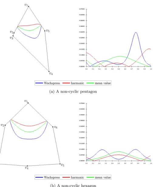
Now let us consider a polygon of irregular shape, where the different barycentric methods have significantly different types of contour lines. In the case of Wach- spress coordinate functions, the contour line curve is closer to those vertices vj, where the area of the triangle Cj (see Figure 1), which is specified by the given vertex vj and its neighborsvj−1, vj+1, is larger. This behavior is clearly visible in Figure 6, where we display some non-cyclic polygons with vertices where the cor- responding area of the triangle is much smaller than neighbouring triangle areas.
Furthermore, it is worth examining the curvature plots of the Wachspress coordi- nate contour lines in these examples, because it shows the behavior of the curve perfectly. In Figure 6a, the area of the triangle C4 at the vertex v4 is evidently larger than the others, thus the curve is predominantly closer to this vertex and the curvature function is increasing on the interval [0.5,0.8] significantly. In the same way, we can observe in Figure 6b that the areas of the triangles C3 andC5
are the same, thus the curve is almost equally close to verticesv3 andv5, but be- cause the area of the triangleC4is very small, the middle part of the curve flattens and it behaves like a straight line. The curvature plot also displays this behavior, because it is almost identical at interval[0.1,0.4]and[0.6,0.9], and the value of it atx= 0.5is close to zero.
The contour line of the harmonic coordinate function is close to the corre- sponding vertexvi, if the anglesβi−1 andγi (see Figure 1) are obtuse. Therefore, in Figure 6a, it behaves contrary to the Wachspress coordinates, because the angles of the polygon at vertices v2and v5 are obtuse. Furthermore, the harmonic coor- dinate method often produces inflection points on the contour line curve in these cases (shown in Figure 6a and 6b).
The mean value coordinate function is more robust than the other methods, as it is clearly visible in all examples of Figure 6.
3.4. Patterns of the barycentric coordinates
In the following examples, we displayed the contour line patterns of the three differ- ent barycentric coordinate functions with respect to the vertexvi, from zero to one by step 0.05. These patterns clearly show the differences between the coordinate functions.
In the case of heavily non-cyclic polygons (see Figure 7a), the three methods produce significantly different patterns. The Wachspress coordinate function pro- vides the most uniform shape of contour line pattern, which we may naively expect from this kind of shapes. We can also see, that there are significantly thicker stripes in the last intervals of the mean value coordinates than in the others, while the stripes of the harmonic coordinate function pattern behave unconventionally, because the upper ones approximate the corresponding vertex vi. This behavior occurs, when the angles of the polygon at the neighbor vertices of the correspond-
(a) A non-cyclic pentagon
(b) A non-cyclic hexagon
Figure 6: Left: Barycentric coordinate functions for non-cyclic polygons with respect to the vertexv1. Right: Curvature plots of
the contour line curves atb1= 0.25
ing vertexvi are obtuse, because if the anglesβi−1+γi > π (see Figure 1), there may be some interior vertices of the polygon the barycentric coordinate of which is negative with respect tovi [14].
Furthermore, if we consider a nearly regular polygon (shown in Figure 7b), we can notice that the Wachspress coordinate method almost behaves like in the
(a) A non-cyclic polygon
(b) A nearly regular polygon
Figure 7: Iso-barycentric contour line patterns of the three different functions with respect to the vertexv1from zero to one by step 0.05
previous figure (see Figure 7a), while the other two work differently, providing more uniform shapes in this case.
4. Affine combination of barycentric functions
As we have seen in the previous sections, each generalized barycentric method has its advantages and drawbacks. For example, discrete harmonic coordinate
functions are based on the minimization of the Dirichlet energy, but provide unusual and irregular shape of contour line patterns. In every application, one has to decide which method fits better to the problem. To overcome this restriction, in this section we introduce the affine combination of barycentric functions. Suppose a polygon P with n vertices is given and the Wachspress coordinates bWi and discrete harmonic coordinates bHi are computed, respectively. Now consider the affine combinationbAi of these coordinates
bAi (λ) = (1−λ)bWi +λbHi ,
where λ ∈ [0,1] is a free parameter. The new coordinates evidently satisfy the requirements formulated in Section 2 to be barycentric coordinates: bAi (λ)≥0 for eachi= 1, ..., n, and the sum of these coordinates is as follows
Xn i=1
bAi (v) = Xn i=1
(1−λ)bWi (v) +λbHi (v)
= (1−λ) Xn i=1
bWi (v) +λ Xn
i=1
bHi (v) = 1.
This affine combination is a tool to merge advantages of two barycentric methods.
The choice of the free parameter λgives us an extra flexibility in order to weight the two methods, which can yield different versions of affine combinations, various trade-offs between uniform patterns and energy minimization, as we can observe in Figure 8.
5. Conclusions
In this paper, we studied the different types of the generalized barycentric co- ordinates (Wachspress, discrete harmonic, mean value) and we compared these functions for convex,n-sided polygons in detail. For the comparison, we used the curvature functions of the contour line curves which are defined by a polynomial fitting algorithm. The curvature functions provided descriptions of the behavior of the contour line curves.
In the case of regular and cyclic polygons, the behavior of the Wachspress and the harmonic coordinate functions is equivalent, and they satisfy the property of variation diminishing, while the mean value coordinates may generate unnecessary inflection points. It is also shown that angle of the polygon at the corresponding vertex heavily affects the different barycentric coordinate methods. The larger the angle, the larger the divergence of the mean value from the other coordinate functions.
With regard to non-cyclic polygons, the three different coordinate methods provide significantly different patterns of contour lines. It can be said generally that the Wachspress coordinates follow the sides of the polygon better, than the others, and provide more uniform patterns, while the harmonic coordinate method behaves unconventionally in some cases, because it produces negative coordinates.
Moreover, we can say that the mean value coordinate function is the most robust for non-cyclic polygons.
(a) Iso-barycentric contour line patterns of Wachspress and discrete har- monic coordinates (top) and their affine combination (bottom) with
λ= 0.12,0.5and0.81, respectively
(b) Contour line curves of Wachspress and harmonic coordinates and their affine combination withλ= 0.22,0.5and0.83, respectively Figure 8: The affine combination of Wachspress and discrete har-
monic coordinate functions with respect to the vertexv1
In order to overcome the shortcomings of these methods, we introduced the affine combination of two barycentric coordinate functions which method also gives us an extra flexibility by the free parameterλ. This way one can provide a trade-off between various advantageous properties and drawbacks of the methods.
References
[1] Möbius, A. F., Der barycentrische calcul, Leipzig, 1827.
[2] Wachspress, E. L., A rational finite element basis, Elsevier, 1975.
[3] Meyer, M., Barr, A., Lee, H., Desbrun, M., Generalized barycentric coordi- nates on irregular polygons,Journal of Graphics Tools, Vol. 7 (2002), 13–22.
[4] Eck, M., DeRose, T., Duchamp, T., Hoppe, H., Lounsbery, M., Stuetzle, W., Multiresolution analysis of arbitrary meshes, Proceedings of SIGGRAPH ’95, (1995), 173–182.
[5] Floater, M. S., Mean value coordinates, Computer Aided Geometric Design, Vol. 20 (2003), 19–27.
[6] Ju, T., Schaefer, S., Warren, J. , Mean value coordinates for closed triangular meshes,ACM Transactions on Graphics (TOG), Vol. 24 (2005), 561–566.
[7] Joshi, P., Meyer, M., DeRose, T., Green, B., Sanocki, T., Harmonic coor- dinates for character articulation, ACM Transactions on Graphics (TOG), Vol. 26 (2007).
[8] Lipman, Y., Levin, D., Cohen-Or, D., Green coordinates,ACM Transactions on Graphics (TOG), Vol. 27 (2008), 78:1–78:10.
[9] Liu, C., Luo, Z., Shi, X., Liu, F., Luo, X., A fast mesh parameterization algo- rithm based on 4-point interpolatory subdivision,Applied Mathematics and Compu- tation, Vol. 219 (2013), 5339–5344.
[10] Morigi, S., Feature-sensitive parameterization of polygonal meshes,Applied Math- ematics and Computation, Vol. 215 (2009), 1561–1572.
[11] Guessab, A., Guessab, F., Symmetrization, convexity and applications, Applied Mathematics and Computation, Vol. 240 (2014), 149–160.
[12] Weber, O., Ben-Chen, M., Gotsman, C., Hormann, K., A complex view of barycentric mappings,Computer Graphics Forum, Vol. 30 (2011), 1533–1542.
[13] Farbman, Z., Hoffer, G., Lipman, Y., Cohen-Or, D., Lischinski, D., Coor- dinates for instant image cloning, ACM Transactions on Graphics (TOG), Vol. 28 (2009), 67:1–67:9.
[14] Floater, M. S., Hormann, K., Kós, G., A general construction of barycentric coordinates over convex polygons,Advances in Computational Mathematics, Vol. 24 (2006), 311–331.
[15] Warren, J., Barycentric coordinates for convex polytopes, Advances in Computa- tional Mathematics, Vol. 6 (1996), 97–108.
[16] Pinkall, U., Polthier, K., Computing discrete minimal surfaces and their conju- gates,Experimental Mathematics, Vol. 2 (1993), 15–36.
[17] Hormann, K., Floater, M. S., Mean value coordinates for arbitrary planar poly- gons,ACM Transactions on Graphics (TOG), Vol. 25 (2006), 1424–1441.
[18] Dyken, C., Floater, M. S., Transfinite mean value interpolation,Computer Aided Geometric Design, Vol. 26 (2009), 117–134.