Optimality of linear factor structures

(1)

Optimality of linear factor structures

by Borbála Szüle

C O R VI N U S E C O N O M IC S W O R K IN G P A PE R S

CEWP 2 /201 7

(2)

Optimality of linear factor structures

Borbála Szüle

^∗

March 14, 2017

Abstract

Factor analysis is often applied in empirical data analysis to explore data structures. Due to its theoretical construction, factor analysis is suitable for the study of linear relationships, and adequacy of a factor analysis solution is often assessed with linear correlation related measures. This paper aims to contribute to literature by examining whether linear factor structures can correspond to multiple require- ments simultaneously. Theoretical and simulation results also suggest that under the applied assumptions the examined optimality criteria can not be met simultaneously. These criteria are related to the determinant of the correlation matrix (that should be minimized so that it is close to zero), the determinant of the anti-image correlation matrix (that should be maximized so that it is close to one), and the Kaiser- Meyer-Olkin measure of sampling adequacy (that should be above a predened minimum value). Results of the analysis highlight the complexity of questions related to the design of quantitative methodology for exploring linear factor structures.

JEL: C43, C52

Keywords: Aggregation, Indicators, Model Evaluation

1 Introduction

Linear factor structures are important in exploring empirical data. Factor analysis, that can provide information about linear factor structures in data analysis, may reveal interesting insights regarding the underlying data pat- terns. If nonlinearity within data does not prevail, factor analysis may be

∗Insurance Education and Research Group, Corvinus University of Budapest, Email:

borbala.szule@uni-corvinus.hu

(3)

applicable for several data analysis purposes. Theoretically a distinction between conrmatory factor analysis (applicable for testing an existing data model) and exploratory factor analysis (aimed at nding latent factors) can be made. (Sajtos-Mitev (2007), pages 245-247) Goodness measures may be related to the specic purpose of a factor analysis, for example the grade of reproducibility of correlations or the size of partial correlation coecients may also contribute to the evaluation of results. This paper focuses on exploratory factor analysis, thus correlation values are of central importance in assessing model adequacy.

Exploratory factor analysis methods include common factor analysis and principal component analysis (Sajtos-Mitev (2007), page 249), with the ma- jor dierence that principal component analysis is based on the spectral decomposition of the (ordinary) correlation matrix, while other factor analysis methods apply dierent algorithms in calculating factors, for example in some cases eigenvalues and eigenvectors of a reduced correlation matrix (as opposed to the unreduced ordinary correlation matrix) are computed. The application of a reduced correlation matrix in calculations (for example in principal axis factoring, that is one of the factor analysis algorithms) em- phasizes the distinction between the common and unique factors that are assumed to determine measurable data. In case of a good exploratory factor analysis output spectral decomposition results in an uneven distribution of eigenvalues so that (relatively easily interpretable) eigenvectors are strongly correlated with observable variables, with partial correlations between measurable variables being relatively low. As a consequence, some criteria (related to the goodness of factor analysis results) can be formulated based on the Pearson correlation coecients and the partial correlation values. The determinant of a correlation matrix is a function of matrix values and thus, although it does not necessarily fully express all information in- herent in the matrix, it can be considered as a simple measure of goodness of factor analysis results. In case of assuming the equality and non-negativity of the o-diagonal elements in a correlation matrix containing Pearson correlation values a lower determinant value indicates a better factor analysis solution. For example if the determinant of this correlation matrix is zero, then some eigenvalues of the correlation matrix are equal to zero and it is possible that all observable variables are perfectly correlated with one of the eigenvectors of the correlation matrix.

Partly similar to Pearson correlation coecients, partial correlation values also describe the linear relationship between two observable variables (while controlling for the eects of other variables). The presence of latent factors in the data may be indicated by linear relationships of observable variables that are characterized by (in absolute terms) high Pearson correla-

(4)

tion coecients and (in absolute terms) low partial correlation values. The total Kaiser-Meyer-Olkin (KMO) value and the anti-image correlation matrix in a factor analysis summarize the most important information about partial correlations. In case of an adequate factor analysis result the total KMO value should be above a predened minimum value (e.g. Kovács (2011), page 95 and George-Mallery (2007), page 256). The o-diagonal elements of the anti-image correlation matrix are the negatives of the partial correlation coecients, while the diagonal values represent partial correlation related measures of sampling adequacy (variable related KMO values) for observable variables. (Kovács (2014), page 156) If the determinant of the anti-image correlation matrix is high (for example close to one) it may be considered as an indicator of the goodness of a factor analysis solution.

The paper aims at exploring whether these alternative goodness criteria can be met simultaneously (the determinant of the ordinary correlation matrix should be close to zero when the determinant of the anti-image correlation matrix is close to one, so that the total KMO value is above the minimum requirement). The key theoretical result of the paper is that if all Pearson correlation coecients between observable variables are assumed to be non-negative values that are equal, then the optimal solutions in case of the two determinants dier. In addition to this, simulation results show that in case of the assumed matrix size, low (close to zero) correlation matrix determinants are not associated with high (close to one) anti-image correlation matrix determinant values if the requirement about the expected minimum of KMO value is also taken into account.

The paper is organized as follows. Section 2 outlines some features of factor analysis methods. Section 3 introduces the assumptions applied to calculate optimality measures, and Section 4 summarizes theoretical and simulation results about optimality criteria in the paper. Section 5 concludes and describes directions for future research.

2 Linear correlation in factor analysis

In exploratory factor analysis the factors can be considered as latent variables that, unlike observable variables, cannot be measured or observed. (Rencher- Christensen (2012), page 435) Interpretable latent variables may not only underlie cross sectional data, but may also be identied in case of time series (Fried-Didelez (2005)). The range of quantitative methods for the analysis of latent data structures is wide, for example conditional dependence models for observed variables in terms of latent variables can also be presented with copulas (Krupskii-Joe (2013)).

(5)

The creation of latent variables can be performed with several algorithms, and a general feature of factor analysis is the central importance of (linear) Pearson correlation values during calculations. According to some authors (e.g. Hajdu (2003), page 386) principal component analysis can be considered as one of the factor analysis methods. However, it has to be emphasized that principal component analysis and other factor analysis methods exhibit certain dierences. In the following these dierences are illustrated with a comparison of principal component analysis and principal axis factoring.

One of the main dierences between these two methods is that in pricipal component analysis the whole correlation matrix can be reproduced if all components are applied for the reproduction, while in principal axis factoring theoretically only a reduced correlation matrix can be reproduced (in which the diagonal values are lower than one). This dierence is related to the dissimilarity of assumptions about the role of unique factors in determining measurable data. Principal axis factoring assumes that common and unique factors are uncorrelated and the diagonal values of the reproduced correlation matrix are related solely to the common factors. In case of principal component analysis the eect of common and unique factors are modeled together. (Kovács (2011), page 89)

Linear combinations of observable variables are called components in principal component analysis, while in principal axis factoring combinations of observable variables are referred to as factors. Despite calculation dierences components and factors (belonging to the same database) may be similar.

The following simulation analysis aims at illustrating similarities of principal component analysis and principal axis factoring results. It is worth mentioning that although factor analysis results are sensitive to outliers (e.g.

Serneels-Verdonck (2008), Hubert et al. (2009)), in the following calculation model, due to the applied distributional assumptions, this possible problem may be considered as not serious.

In data analysis, simulations may be applied to assess selected features of algorithms (Josse-Husson (2012)), for example related to factor analysis (Brechmann-Joe (2014)). Assume that the matrix containing theoretical Pearson correlation values is described by Equation (1).

R =





1 r₁ r₂ r₁ 1 r₃ r₂ r₃ 1



 (1)

Based on Equation (1) it is possible to simulate empirical correlation matrices by means of the Cholesky decomposition of the correlation matrix

(6)

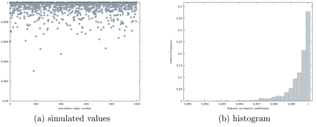
(a) simulated values (b) histogram

Figure 1: Simulated Pearson correlation values Source: own calculations

(R = C · C^T), with the transformation of independent normal variables into dependent normal (Madar (2015)). The matrix C in this Cholesky decomposition is described by Equation (2).

C =







1 0 0

r₁ p

1−r²₁ 0 r₂ ^r√³^−r¹^·r²

1−r₁²

q

1−r²₁− ^(r³^−r_1−r¹^·r2)2 ² 1





 (2)

In the simulation analysis it is assumed that 1000 observations belong to each of the three variables, and these variables follow a normal distribution.

The number of simulations is 1000. Related to these distributional assumptions it is worth mentioning that (as Boik (2013) points out) it is possible to construct principal components without assuming multivariate normality of data. For each set of simulated variables principal component analysis and principal axis factoring are performed and the component and factor with the highest eigenvalue is calculated. If the absolute value of Pearson correlation between this component and this factor is close to one in a simulation, then it can be considered as indicating the similarity of principal component analysis and factor analysis results. Since the components and factors correspond to eigenvectors, thus the absolute values of correlation coecients are analyzed. In a relatively simple example it can be assumed that r₁ = 0,r₂ = 0 and r₃ = 0.99. Simulated Pearson correlation values and the histogram (belonging to this example) are illustrated by Figure 1.

The distribution of Pearson correlation coecients (between the component and the factor) indicate that the simulated values are relatively close to one, thus in this example principal component analysis and principal axis

(7)

factoring results can be considered as relatively similar. The appendix introduces simulation results for three additional examples, and the similarity of principal component analysis and factor analysis results can be observed also in case of these examples: the correlation values between the component and the factor in the examples are relatively close to one. Thus (although the theoretical construction of principal axis factoring is more appropriate in identifying latent factors in data) in the following it is assumed that the spectral decomposition of the complete (unreduced) correlation matrix can also provide information about the goodness of factor analysis results, and in the following the complete (unreduced) correlation matrix is applied in the calculations (instead of a reduced correlation matrix).

3 The correlation model

An ordinary correlation matrix can be quite complex, since the only theoretical restriction related to its form is that it is a symmetric positive semidenite matrix. Strong (Pearson) correlations between observable variables and latent factors (calculated with the application of factor analysis algorithms) are often considered as indicating a good linear factor structure, but it is worth emphasizing that low partial correlations between observable variables are also necessary to the identication of latent factors. The question arises whether there is a linear factor structure that corresponds to all these re- quirements. The paper aims at contributing to the research of this question.

Since the potential complexity of a correlation matrix increases with its size, the paper examines a simple case with three observable variables. Even in this case the requirement that the (ordinary) correlation matrix is positive semidenite allows several combinations of (Pearson) correlation values. As- sume for example that the correlation matrix is dened as in Equation (1).

The requirement that the (ordinary) correlation matrix is positive semidef- inite is equivalent to assuming that the correlation matrix has only nonnegative eigenvalues. Assume that the lowest eigenvalue of the correlation matrix in Equation (1) is indicated by λ₃, then it can be calculated based on Equation (3):

(1−λ₃)³−(1−λ₃)·(r₁²+r₂²+r₃²) + 2·r₁·r₂·r₃ = 0 (3) Theoretically the solution of Equation (3) could be a complex number (and then its interpretation in factor analysis could be problematic), but since all values in the correlation matrix are real numbers, thus the eigenvalues of the correlation matrix are also real numbers. As a solution of Equation (3)

(8)

the lowest eigenvalue of the correlation matrix in Equation (3) is described by Equation (4):

λ3 = 1−2·

rr²₁+r²₂+r²₃ 3 ·cos





 1

3 ·arccos







−r₁·r₂·r₃ r_r2

1+r₂²+r²₃ 3

3











 (4)

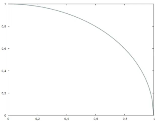
To illustrate that only certain combinations of correlation values are related to a positive semidenite correlation matrix, assume in the following example that r₁ = 0. In case of this assumption Equation (4) is equivalent to Equation (5):

λ₃ = 1−2·

rr²₁+r₂²+r₃²

3 ·cosπ 6

(5)

By rearranging Equation (5) the condition for the positive semideniteness of the correlation matrix is described by Equation (6):

q

r²₂ +r₃² ≤1 (6)

The possible combinations of correlation values that meet the condition in Equation (6) are illustrated by Figure 2, on this graph all combinations of Pearson correlations (indicated on the horizontal and vertical axis of the graph) that are not above the plotted curve result in a semidenite ordinary correlation matrix.

These results indicate that, as a consequence of the theoretical positive semideniteness of the correlation matrix, the relationships of Pearson correlation values in an (ordinary) correlation matrix should meet some re- quirements. For the sake of simplicity, in the following it is assumed that all o-diagonal elements in the ordinary correlation matrix are non-negative values that are equal: r₁ =r₂ =r₃ =r and r >= 0. In this case the lowest eigenvalue in Equation (3) is equal to1−r (under these simple assumptions the highest eigenvalue of the ordinary correlation matrix is equal to 1 + 2r, and the other two eigenvalues are equal to 1−r), thus the condition for the positive semideniteness of the correlation matrix is met. In the following

(9)

Figure 2: Possible combinations of correlation values Source: own calculations

theoretical results are calculated under these simple assumptions about the form of the ordinary correlation matrix.

4 Correlation based optimality measures

Goodness of an explanatory factor analysis solution has several aspects, thus the range of possible goodness measures is also relatively wide. For example with the application of Barlett's test it may be evaluated whether the sample correlation matrix diers signicantly from the identity matrix (Knapp-Swoyer (1967), Hallin et al. (2010)) when all eigenvalues were equal (and thus the related eigenvectors could not be interpreted as correspond- ing to latent factors). Theoretically subsphericity (equality among some of the eigenvalues) could also be tested (Hallin et al. (2010)), and other eigenvalue related goodness of t measures (Chen-Robinson (1985)), for example the total variance explained by the extracted factors (Martínez-Torres et al. (2012)), Hallin et al. (2010)) may also contribute to the assessment of factor models. Beside these aspects, interpretability of factors is an other important question in goodness evaluation (Martínez-Torres et al. (2012)), that should be considered when deciding about the number of extracted factors. The choice of relevant factors (or for example components in a principal component analysis) may depend also on the objectives of the analysis (Ferré (1995)) If maximum likelihood parameter estimations can be performed, then for example Akaike's information criterion (AIC) or Bayesian information cri-

(10)

terion (BIC) may be applied during the determination of the factor number (Zhao-Shi (2014)), but it is worth emphasizing that not all factor selecting approaches are related to distributional assumptions (Dray (2008)), for example a possible method for factor extraction is to retain those factors (or components) that have eigenvalues larger than one (Peres-Neto (2005)). De- spite the wide range of possible goodness measures, the comparison of factor analysis results is not necessarily simple, since factor loadings in dierent analyses can not be meaningfully compared. (Ehrenberg (1962))

In the following a simple theoretical model is introduced, in which the relationship of selected goodness measures is analyzed. It has to be emphasized that although theoretically a distinction could be made between data adequacy (for example whether correlation values make data aggregation possible) and goodness of factor analysis results (for example whether factors can be easily interpreted), this paper does not analyze potential diculties in the interpretation of factors, thus data adequacy and goodness of factor analysis results can be considered as similar concepts in the paper.

Goodness of a factor structure can be evaluated based on ordinary and partial correlations, thus in the following these values are calculated in a theoretical model. Equation (7) contains the (symmetric and positive semidenite) ordinary correlation matrix that corresponds to the simple assumptions in the paper.

R =





1 r r r 1 r r r 1



 (7)

These assumptions result in a nonnegative positive semidenite matrix, and although an exact nonnegative decomposition of a nonnegative positive semidenite matrix is not always available (Sonneveld et al. (2009)), the eigenvalues are all nonnegative real numbers in this case.

Under the applied simple assumptions the determinant of the ordinary correlation matrix is described by Equation (8), as also presented by the literature (e.g. Joe (2006)).

det(R) = 2·r³−3·r²+ 1 (8) Theoretically the determinant of a correlation matrix can be between zero and one, and the determinant of the unity matrix is equal to one. If the

(11)

correlation matrix is a unity matrix, then all eigenvalues of the correlation matrix are equal to one, and in a factor analysis this case would correspond to a solution, when the highest number of observable variables that strongly correlate with a calculated factor is only one. Thus, if the correlation matrix is a unity matrix, factor analysis solutions can not be considered as optimal.

Based on these considerations, a lower (close to zero) correlation matrix determinant could indicate a better factor structure (that could be related to latent factors in data). In this paper, one of the factor structure optimality criteria is dened in terms of the ordinary correlation matrix determinant:

the factor structure that belongs to the lowest correlation matrix determinant is identied as optimal from this point of view.

An other aspect of the optimality of factor structures is related to the partial correlation coecients between the observable variables. Partial correlations measure the strength of the relationship of two variables while controlling for the eects of other variables. In a good factor model the partial correlation values are close to zero. (Kovács (2011), page 96) The anti-image correlation matrix summarizes information about the partial correlation coecients: the diagonal values of the anti-image correlation matrix are the Kaiser-Meyer-Olkin (KMO) measures of sampling adequacy, and the o-diagonal elements are the negatives of the pairwise partial correlation coecients. The KMO measure of sampling adequacy can be calculated for the variables separately, or for all variables together. If calculated for the variables separately (and if pairwise Pearson correlation values and partial correlation coecients are indicated by r_ij and p_ij, respectively), the KMO value is equal to

P

i6=j

rij2

P

i6=j

rij2+P

i6=j

pij2. (Kovács (2011), pages 95-96) Equation (9) shows the anti-image correlation matrix that corresponds to the model assumptions:

P =





KM O −p −p

−p KM O −p

−p −p KM O



 (9)

Theoretically the maximum value in case of the KMO measure is equal to one (if the partial correlation values were equal to zero), and a higher KMO value indicates a better database for the analysis (Kovács (2011), pages 95- 96) Similar to the individual KMO values that can be calculated for the variables, the total (database level) KMO value (that takes into account all pairwise ordinary and partial correlation coecients) can also be calculated:

(12)

P

i6=j

Prij2

P

i6=j

Prij2+P

i6=j

Ppij2. In case of an adequate factor analysis solution the total KMO value should be at least 0.5. (Kovács (2011), page 95 and George- Mallery (2007), page 256)

Under the assumptions in the paper the pairwise partial correlation coef- cients are equal in the simple model framework, and can be expressed as a function of the Pearson correlation values, as described by Equation (10).

p= r

r+ 1 (10)

The variable-related KMO values are also equal for each variable and this KMO value is described by Equation (11).

KM O= (1 +r)²

(1 +r)²+ 1 (11)

As indicated by Equation (12), based on Equation (10) and Equation (11) the determinant of the anti-image correlation matrix can be expressed as a function of the Pearson correlation values (indicated by r in the model).

det(P) = (1 +r)² (1 +r)²+ 1

!3

−2· r³

(1 +r)³ −3· (1 +r)²

(1 +r)²+ 1 · r²

(1 +r)² (12)

Theoretically, as far as partial correlation values are concerned, in case of an optimal factor structure the pairwise partial correlation coecients were equal to zero, thus also resulting in all KMO values being equal to one.

In this optimal case the anti-image correlation matrix were a unity matrix with a determinant equal to one. Based on these considerations, an other optimality criterion can be dened in terms of the determinant belonging to the anti-image correlation matrix: the optimal factor structure is associated with the highest determinant value (that should be close to one). It is worth mentioning that theoretically the determinant of the anti-image correlation matrix can not only be a value between zero and one.

(13)

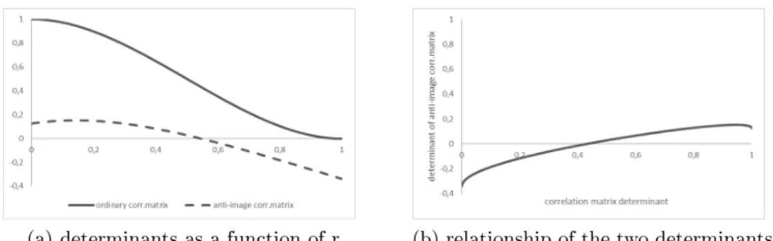
(a) determinants as a function of r (b) relationship of the two determinants

Figure 3: Correlation matrix determinants Source: own calculations

It has to be emphasized that optimality is only analyzed from a math- ematical point of view in this paper (whether goodness criteria can be met simultaneously), but in practical applications other aspects (for example interpretability) may also contribute to the identication of an optimal factor structure. In the paper only the two correlations matrix determinants are compared and the requirement about the total KMO value is analyzed.

Figure 3 shows the determinants as a function of the Pearson correlation (indicated by r in the model) and illustrates the relationship of the two matrix determinants. It can be observed that the minimal correlation matrix determinant value belongs to that case when the Pearson correlation between the variables is equal to one. The determinant of the anti-image correlation matrix reaches its maximum at a Pearson correlation value that is lower than one. These results indicate that in this simple example the two optimality criteria (dened in terms of the matrix determinants) can not be met simultaneously. Results also show that the determinant of the anti-image correlation matrix is not close to one, thus this goodness requirement is also not met. In addition to these results, in this case the requirement about the total KMO value (that it should be at least 0.5) does not have an eect on the conclusion about the availability of factor solutions that simultaneously correspond to multiple goodness criteria, since (as Figure 3 shows) under the applied simple theoretical assumptions no factor structure corresponds to the goodness criteria (described by the correlation matrix determinants) simultaneously.

Although these conclusions belong to a relatively simple case, the results may also indicate potential diculties in nding linear factor structures that are adequate not only from the point of view of Pearson correlation coecients, but also in terms of partial correlation values (that are important in deciding whether a linear combination of observable variables can be consid-

(14)

(15)

5 Conclusions

With the development of information technologies the amount of empirically analyzable data has grown continuously over the last decades. Along with these tendencies, the need for advanced pattern recognition techniques has also increased. Linear factor structures may be present in data, and theoretically several factor analysis methods can be applied to identify latent factors. It is thus a compelling research question, whether theoretically there are optimal linear factor structures.

Factor analysis methods are related to the measurement of strength of linear relationships between observable variables. The ordinary correlation matrix contains information about linear relationships between variables, this matrix however can be quite complex, since the only theoretical restriction about its form is that it is symmetric and positive semidenite. Partly as a consequence of the complexity of correlation matrices various optimality criteria can be formulated for the evaluation of factor analysis results. In addition to the requirement about the Kaiser-Meyer-Olkin measure of sampling adequacy (it should be above a minimum value), this paper denes optimality in terms of two matrices (the ordinary correlation matrix and the anti-image correlation matrix), with the formulation of two theoretical optimality criteria (minimization of the determinant of the ordinary correlation matrix and maximization of the determinant of the anti-image correlation matrix), by also taking into account that for a good factor analysis solution the determinant of the ordinary correlation matrix should be close to zero, while the determinant of the anti-image correlation matrix should be close to one. Relevancy of the anti-image correlation matrix (that contains information about partial correlations) is explained by the importance of (in absolute value) low partial correlations in identifying linear combinations of observable variables as latent factors.

The paper aims at contributing to the literature with a simultaneous analysis of the applied goodness criteria in case of a relatively small correlation matrix (that has 3 columns), by presenting both theoretical and simulation results. Despite the relative simplicity of theoretical model assumptions and optimality criteria denition, the results may provide interesting insights into the relationship of Pearson correlation coecients and partial correlation values. Theoretical results suggest that the two optimal factor solutions (that correspond to the maximization of the anti-image correlation matrix deter-

(16)

minant and the minimization of the ordinary correlation matrix determinant) are not identical, and the maximum determinant value of the anti-image correlation matrix (under the simple model assumptions) is not close to one.

Simulation results illustrate that the determinant related optimality criteria (that the anti-image correlation matrix determinant should be close to one while the ordinary correlation matrix determinant is close to zero) can not be met simultaneously, when the KMO value related requirement is also taken into account. These results are associated with the relationship of the Pear- son correlation values (between observable variables) and the pairwise partial correlation coecients: the theoretical model illustrates that an increase in the pairwise Pearson correlation values may be related with an increase in the partial correlation coecients.

Optimality of linear factor structures has several aspects, thus its further analysis oers a wide range of directions for future research. Possible theoretical extensions of the model in the paper include for example modications in the denition of optimality criteria, or a more general set of assumptions about the elements in the ordinary correlation matrix.

References

[1] Boik, R. J. (2013): Model-based principal components of correlation matrices. Journal of Multivariate Analysis 116, pp. 310-331.

[2] Brechmann, E. C. Joe, H. (2014): Parsimonious parameteriza- tion of correlation matrices using truncated vines and factor analysis.

Computational Statistics and Data Analysis 77, pp. 233-251.

[3] Chen, K. H. Robinson, J. (1985): The asymptotic distribution of a goodness of t statistic for factorial invariance. Journal of Multivariate Analysis 17, pp. 76-83.

[4] Dray, S. (2008): On the number of principal components: a test of dimensionality based on measurements of similarity between matrices.

Computational Statistics & Data Analysis 52, pp. 2228-2237.

[5] Ehrenberg, A.S.C. (1962): Some questions about factor analysis.

Journal of the Royal Statistical Society. Series D (The Statistician) 12(3), pp. 191-208.

(17)

[6] Ferré, L. (1995): Selection of components in principal component analysis: a comparison of methods. Computational Statistics & Data Analysis 19, pp. 669-682.

[7] Fried, R. Didelez, V. (2005): Latent variable analysis and partial correlation graphs for multivariate time series. Statistics & Probability Letters 73, pp. 287-296.

[8] George, D. Mallery, P. (2007): SPSS for Windows Step by step.

Pearson Education, Inc.

[9] Hajdu, O. (2003): Többváltozós statisztikai számítások. Központi Statisztikai Hivatal, Budapest (in Hungarian)

[10] Hallin, M. Paindaveine, D. Verdebout, T. (2010): Optimal rank-based testing for principal components. The Annals of Statistics 38(6), pp. 3245-3299.

[11] Hubert, M. Rousseeuw, P. Verdonck, T. (2009): Robust PCA for skewed data and its outlier map. Computational Statistics and Data Analysis 53, pp. 2264-2274.

[12] Joe, H. (2006): Generating random correlation matrices based on partial correlations. Journal of Multivariate Analysis 97, pp. 2177-2189.

[13] Josse, J. Husson, F. (2012): Selecting the number of components in principal component analysis using cross-validation approximations.

Computational Statistics and Data Analysis 56, pp. 1869-1879.

[14] Knapp, T. R. Swoyer, V. H. (1967): Some empirical results con- cerning the power of Bartlett's test of the signicance of a correlation matrix. American Educational Research Journal 4(1), pp. 13-17.

[15] Kovács, E. (2014): Többváltozós adatelemzés. Typotex (in Hungarian) [16] Kovács, E. (2011): Pénzügyi adatok statisztikai elemzése. Tanszék

Kft., Budapest (in Hungarian)

[17] Krupskii, P. Joe, H. (2013): Factor copula models for multivariate data. Journal of Multivariate Analysis 120, pp. 85-101.

[18] Madar, V. (2015): Direct formulation to Cholesky decomposition of a general nonsingular correlation matrix. Statistics and Probability Let- ters 103, pp. 142-147.

(18)

[19] Martínez-Torres, M.R. Toral, S.L. Palacios, B. Bar- rero, F. (2012): An evolutionary factor analysis computation for min- ing website structures. Expert Systems with Applications 39, pp. 11623- 11633.

[20] Peres-Neto, P. R. Jackson, D. A. Somers, K. M. (2005):

How many principal components? stopping rules for determining the number of non-trivial axes revisited. Computational Statistics & Data Analysis 49, pp. 974-997.

[21] Rencher, A. C. Christensen, W. F. (2012): Methods of Multi- variate Analysis. Third Edition, Wiley, John Wiley & Sons, Inc.

[22] Sajtos, L. Mitev, A. (2007): SPSS kutatási és adatelemzési kézikönyv. Alinea Kiadó, Budapest (in Hungarian)

[23] Serneels, S. Verdonck, T. (2008): Principal component analysis for data containing outliers and missing elements. Computational Statistics & Data Analysis 52, pp. 1712-1727.

[24] Sonneveld, P. van Kan, J.J.I.M. Huang, X. Oosterlee, C.W. (2009): Nonnegative matrix factorization of a correlation matrix.

Linear Algebra and its Applications 431, pp. 334-349.

[25] Zhao, J. Shi, L. (2014): Automated learning of factor analysis with complete and incomplete data. Computational Statistics and Data Anal- ysis 72, pp. 205-218.

(19)

Appendix

Comparison of eigenvectors in principal component analysis and principal axis factoring

In the following example three cases are analyzed. Similar to Section 2, in each of these cases it is assumed that the theoretical Pearson correlation coecients are described by Equation (1).

For each of the three analyzed cases it is assumed that the variables (with 1000 observations) in the analysis follow a normal distribution. The number of simulations is 1000 in each of the cases. For each simulation principal component analysis and principal axis factoring are performed and the component and factor with the highest eigenvalue is calculated. An adequately high (close to one) absolute value of the Pearson correlation between this component and this factor can be considered to indicate similarity of principal component analysis and principal axis factoring results. The empirical distribution of these Pearson correlation values is analyzed and compared among the three cases (the absolute values of correlation coecients are analyzed, since these components and factors correspond to eigenvectors). In the analyzed three cases it is assumed that r₁ = r₂ = r₃ so that the theoretical correlation in the examples is 0.25, 0.75 and 0.99, respectively. The following gures (showing the simulated Pearson correlation coecients and the histogram of these correlation values) illustrate dierences in these cases.

The main conclusion is that in these simulation examples the results of principal component analysis and principal axis factoring can be considered as relatively similar, since the Pearson correlation coecients (in absolute value) between the component and factor with the highest eigenvalue are relatively close to one. According to simulation results that are summarized in the following table, the standard deviation of these values is smaller if the correlation values are larger in the theoretical correlation matrix.

correlation values average st. dev.

r = 0.25 0.996788 0.003481 r = 0.75 0.999785 0.000228 r = 0.99 0.999995 0.000005

(20)

(a)r= 0.25, simulated values (b)r= 0.25, histogram

(c)r= 0.75, simulated values (d)r= 0.75, histogram

(e)r= 0.99, simulated values (f)r= 0.99, histogram

Simulation results Source: own calculations