Trade impacts of the New Silk Road in Africa: Insight from Neural Networks
Analysis
KOFFI DUMOR, Ph.D.
SCHOLAR
UNIVERSITY OF ELECTRONIC SCIENCE AND
TECHNOLOGY OF CHINA e-mail: dumor3000@yahoo.fr
KOMLAN GBONGLI, Ph.D.
RESEARCHER
UNIVERSITY OF MISKOLC e-mail: samxp12@yahoo.fr
pzkgbong@uni-miskolc.hu
SUMMARY
The Belt and Road Initiative (BRI) is aimed to strengthen the preferential reciprocal trade between China and the Belt- Road nations. Quantitative evaluations of BRI to determine whether it can explicitly provide more insight into China’s bilateral trade among its partners are needed. Hence, improving prediction accuracy while using more superior algorithms for sustainable decision-making remains essential since decision-makers have been interested in predicting the future. Machine learning algorithms, such as supervised artificial neural networks (ANN), outperform several econometric procedures in predictions; therefore, they are potentially powerful techniques to evaluate BRI. This study uses detailed China’s bilateral export data from 1990 to 2017 to analyze and evaluate the impact of BRI on bilateral trade using gravity model estimations and ANN analysis techniques. The finding suggests that China’s bilateral export flow among the BRI countries results in a slight increase in inter-regional trade. The study provides a comparison view on the different estimation procedures of the gravity model – ordinary least squares (OLS) and Poisson pseudo- maximum likelihood (PPML) with the ANN. The ANN associated with fixed country effects reveals a more accurate estimation compared to a baseline model and with country-year fixed effects. Contrarily, the OLS estimator and PPML showed mixed results. Grounded on the study dataset, the ANN estimation of the gravity equation was superior over the other procedures to explain the variability of the dependent variable (export) regarding the prediction accuracy using root mean squared error (RMSE) and R-square.
Keywords: China’s Belt and Road Initiative; Bilateral Trade; Gravity Model; Artificial Neural Network methodology;
African Countries.
Journal of Economic Literature (JEL) codes: B17; F14; N77 DOI: http://dx.doi.org/10.18096/TMP.2021.03.02
I NTRODUCTION
The Belt and Road Initiative (BRI), regarded as
“China’s grand connectivity blueprint,” remains the most ambitious economic project that China has introduced since 2013 (Chung, 2018) (Khan et al., 2018) (Flint & Zhu, 2019). This project is designed to promote economic growth by reinforcing inter-regional cooperation over a vast area entailing sub-regions in Asia, Europe, and Africa. It has emphasized five priorities for China and the BRI participating nations, including policy coordination, unimpeded trade, facility connectivity, financial integration, and the bond
between people (Khan et al., 2018). Moreover, the project target to support infrastructure, trade, and investment links between China and some 65 other nations that can reach together over 30% of global GDP, 62% of the population, and 75% of known energy reserves (Huang, 2016). Therefore, the BRI initiative brings about a greater diversity of trade partners and trade patterns, giving the industry new opportunities to transform and upgrade itself.
Throughout the past seven years, China’s economic cooperation with the Belt-Road countries has attained substantial results. In the same vein, the bilateral trade between China and Belt-Road countries has considerably improved. As such, the total trade value
of goods between China and Belt-Road countries had exceeded $7.8 trillion from 2013 to 2019, grounded on the data revealed by the Ministry of Commerce of China (China’s Trade with BRI Countries Surges to
$1.34 Trillion in 2019, 2020). The Belt and Road Initiative, with unimpeded trade as one crucial objective, has become a principal new-round opening up plan and is considered as a tool for boosting China’s foreign trade, especially with countries along the BRI (Boffa, 2018). Considering the indicated intention to encourage trade flows among economies included in the BRI, bilateral trade flow is an important economic indicator adopted by economists and policy-makers. It explains the value of goods and services that have been exported from one country to another, inducing international trade policy along with domestic economic policy in both countries.
Supporters stress that the New Silk Road, or BIR initiative, allows building novel infrastructure and providing economic assistance to needy economies.
Critics of the projects argue that the initiative instead eases the Chinese economic and strategic dominion over the countries along these routes. However, trade facilitation may mitigate transaction costs, simplify trade procedures, and improve customs efficiency as a common rule (Moïsé & Sorescu, 2013). Earlier studies that have attempted to build analysis systems for trade facilitation vary significantly regarding the indicators to be used. From this perspective, Raven (2001) argued that the indicators should include the customs environment, payment system efficiency, and business credibility. For Wilson et al. (2003), the indicators comprised four elements: port efficiency, customs environment, institutional environment, and e- commerce to find their evaluation system. Li & Duan (2014) selected six indicators, entailing port efficiency, customs environment, institutional environment, business environment, e-commerce, and market access, into the evaluation system, and used the entropy method to compute the trade facilitation scores of 109 countries in the World. Zhu & Lu (2015) used indicators based on five areas, including infrastructure and services, port efficiency, customs environment, information and communication technologies, and business environment, then adopted the Delphi method and analytic hierarchy process (AHP) to determine the weight of each indicator.
In connection with these, integrating a multi- analytic technique revealed how merging two diverse data analysis approaches in either methodology or analysis can support the validity and confidence in the output (Gbongli, 2017; Gbongli et al., 2019; Scott &
Walczak, 2009; Gbongli et al., 2020). Regarding the various methods, a series of gravity models or computable general equilibrium (CGE) models have been extensively adopted to assess the effect of trade facilitation on trade flows (Dennis, 2006; Iwanow &
Kirkpatrick, 2009; ZAKI, 2014). For instance, Y. B.
Zhang & Liu (2016) took the extended trade gravity model to research the trade facilitation along “the Silk
Road Economic Belt.” Their finding showed a U- shaped distribution since Europe has demonstrated the highest levels of trade facilitation, east Asia revealed the middle levels. In contrast, countries in the middle of the belt presented the lowest levels, and the impact of trade facilitation on diverse regions disclosed notable heterogeneity (Y. B. Zhang & Liu, 2016).
Traditionally, the multiplicative gravity model has been linearized and evaluated using either ordinary least squares (OLS) to assume that the error variance is constant across observations (homoscedasticity) or using panel techniques that the error is constant across countries as an alternative country-pairs. However, as Santos et al. (Silva & Tenreyro, 2006), when the issues of heteroscedasticity arise, OLS estimation may not be consistent and non-linear estimators should be adopted.
From this end, the combined methodology such as gravity model and artificial neural network (ANN) was applied in human mobility, particularly to predict human mobility within cities based on traditional and Twitter data (Pourebrahim et al., 2018) to compare their performance and results. Conversely, there is a lack of this technique in studying bilateral trade flow amongst various countries. During the last decades, with the fast advancements in computer and information communication technologies (ICTs), adopting artificial intelligence-based techniques in time series or panel data forecasting has become a common practice among researchers. Analytical methods that embody complex computational algorithms may offer the most practical approach for assessing a multivariate response of a BIR project amongst various countries.
Mainly, neural network models use computer-based learning methods that mimic the human brain's neuronal structure (Garson, 1991; Ripley, 1996).
Therefore, artificial neural network-based models could predict international trade estimation as a promising forecasting tool.
In light of the above discussion, this paper aims to offer a quantitative analysis of the existing bilateral export linkages among economies regarding gross trade, mainly the bilateral trade flow between China and African Countries. Since the BRI is presented as an open arrangement in which all countries are welcome to participate, there is no official list of “BRI countries.”
Different versions of unofficial lists of countries along the Belt and Road exist, none of which received confirmation from China (Boffa, 2018). The study proposes evaluating and predicting this bilateral trade using the hybrid methodology such as gravity model and ANNs. The non-linear and non-parametric model (i.e., ANN) is mainly assessed against the international model estimated using OLS regression and Poisson Pseudo Maximum Likelihood (PPML) precisely. The input to our algorithms is a set of economic and geographic variables as well as regional trade agreements, such as GDP, distance, and infrastructure between the importer and exporter countries. Our input space will be discussed extensively in the feature section. We use linear regression with raw and
logarithmic features, kernelized linear regression, and a neural network with various architectures. The output of these algorithms is the bilateral export value measured in billion U.S. dollars ($). The study intends to offer new insights into African policy-makers in charge of relations with China. Holslag (2017) stressed that an assessment of the BRI and the objectives and tools to improve it is undoubtedly crucial for academic debates about the international political economy.
This research contributes to understanding the potential impacts of further opening up of the Chinese economy with the development of BRI practice. It is added to the various effects of BRI on improving developing countries’ exports to high-profit markets.
Academically, this is amongst the central attempts to adopt the combined gravity model and artificial neural model in assessing the potential effect of trade liberalization on the Chinese economy, making room for the future economic analysis of the BRI project. In doing so, this research provides an alternative to time- series predictions and expert judgment assessment by relying on neural networks and boosting methodologies that enable alternative and robust specifications of complex economic relationships (Baxter, 2017).
The remainder of the paper is structured as follows:
The following section provides the literature on bilateral trade associated with the combined method viewed as related work. Section 3 gives an overview of gravity and neural network models; Section 4 introduces the data sources and methodology; Section 5 presents the analysis and discussion, including neural network predictions with actual trade among China and its selected BRI members. In the final section, the conclusion remark entailing implications and future research are discussed.
L ITERATURE REVIEW
This section discusses the standard gravity model and neural networks estimation on bilateral trade perspectives among the member countries of the BRI.
The section highlights different methods used by studies that put the trade effects of the BRI at the center of their investigation. This is to justify the application of augmented gravity and neural networks estimation in this study.
Since Tinbergen (1962) and Pöyhönen (1963) published critical articles, many implementations of the gravity model of international commerce have been suggested in the literature (Yotov et al., 2016). In its reduced form, the gravity equation demonstrates how the value of trade flows between two nations is directly proportional to their economic size and inversely proportional to their distance and other variables influencing the cost of bilateral commerce, such as trade regulations. At first, the gravity model's empirical effectiveness in describing the geographical distribution of commerce was accompanied by a dearth of theoretical backing. Following Anderson's (1979)
work, many writers developed a variety of theoretically grounded versions of the model (Bergstrand, 1989);
Deardorff (1998); Eaton & Kortum (2002). Anderson
& van Wincoop (2003) proposed an enhanced gravity equation that included variables for multilateral trade resistance (MTR). These words convey the notion that trade flows between two nations are determined not just by their bilateral trade resistance (i.e., trade costs associated with distance and other bilateral trade obstacles), but also by the expenses associated with dealing with each country's other trading partners (MTR). Neglecting MTR in the gravity equation is referred to as a "gold medal error" (Baldwin &
Taglioni, 2006), which may be avoided using a variety of econometric methods (Yotov et al., 2016). Feenstra (2015) suggested the use of country-specific fixed effects, Baier & Bergstrand (2009) used a first-order Taylor series approximation to account for MTR, and, more recently, Metulini et al. (2018) posited the use of origin- and destination-specific spatial filters.
Among recent studies on the association between trade and infrastructure, Donaubauer et al. (2018) modified Feenstra et al.'s, (2001) approach to examine the effect of infrastructure on bilateral trade between 150 established and developing countries. In a similar vein, Lee & Itakura (2018) and Kim & Mariano (2020) examined the effect of increased infrastructure on China's trade with Central Asian nations and the impact of infrastructure quality on bilateral trade ties in the Central Asia Regional Economic Cooperation (CAREC) area, respectively. Herrero & Xu (2017) examined the impact of infrastructure investment on trade-in BRI-eligible countries, using the model specification proposed by Baier & Bergstrand (2009) and Hussain et al. (2019) used the same methodology to examine the relationship between exports and infrastructure indicators in 46 Asian countries.
Although there is a substantial body of literature on gravity models, the use of machine learning techniques such as artificial neural networks (ANNs) to predict trade flows remains a novel field of study (Dumor &
Yao (2019), Gopinath et al., 2021). Studies have compared the forecasting performance of ANNs with univariate time series models, macroeconomic fundamentals-based models estimated by ordinary least squares (OLS), and multivariate time series models.
Wu (1995), G. P. Zhang (2003), and Khashei et al.
(2013) compared the forecasting performance of autoregressive integrated moving average (ARIMA) models and ANNs in terms of RMSE and MAE. The ANNs performed substantially better than the ARIMA models. Lisi & Schiavo (1999) and Leung et al. (2000) employed ANNs for forecasting various exchange rates concerning the Random Walk (R.W.) model by adopting normalized mean square error (NMSE) and RMSE as performance criteria.
In their study, Wohl & Kennedy (2018) exhibited an extremely starter endeavor to examine international trade with neural networks and the traditional trade gravity model approach. The findings showed that the
neural network has high prediction accuracy compared to RMSE within the gravity model. Further, Athey (2018), in his research paper, presented an appraisal of the early commitments of machine learning to economics, and likewise, expectations about its future contribution. He also investigated a few features from the developing econometric consolidating machine learning and causal inference, including its impacts on the nature of collaboration on research tools and research questions. A research work performed by Nummelin & Hänninen (2016) utilized the support vector machine (SVM) to break down and conjecture reciprocal exchange streams of soft sawn wood.
More applicable to our target, Nuroglu (2014) demonstrated that neural networks achieve a lower MSE when contrasted with panel data models by using data from 15 E.U. countries. Tkacz & Hu (1999) also showed that financial and monetary variables could be improved using artificial neural network (ANN) techniques. Given the combined ANN and market microstructure approaches to investigate exchange rate fluctuations, the work of Gradojevic & Yang (2000) revealed that macroeconomic and microeconomic variables are valuable to forecast high-frequency exchange rate variations. Similarly, Varian (2014) and Circlaeys et al. (2017) provided an overview of machine learning tools and techniques, including their effect on econometrics. Furthermore, Bajari et al.
(2015) presented an overview and applied a few statistics and computer science methods to issues of interest estimation. The findings showed that machine learning combined with econometrics anticipates the request out of the test in standard measurements considerably more precisely than a panel data model.
As departing from the earlier works, the ANN techniques are applied to the gravity model of bilateral trade flows in this study. The gravity model is often discussed as the workhorse in international trade since its popularity and success in quantifying the effects of various determinants of international trade. Therefore, the two-stage approaches are adopted by estimating and forecasting China’s export with a New Silk Road Initiative member countries using a large dataset from UN-Comtrade that includes 163 countries based on the two-stage approaches gravity model-ANN analysis.
R ESEARCH MODEL Gravity Models
Initiated by Pöyhönen (1963) and Salette &
Tinbergen (1965), the gravity model is one of the most successful empirical approaches in trade. Longtime remained with the traditional economic theories of trade; the gravity model is now deeply integrated with the theoretical foundations in economics with literature rich in contributions and perspective (Anderson & Van
Wincoop, 2003). Gravity models are regarded as a workhorse technique of international trade analysis.
Their fundamental perception is that trade between two countries is anticipated to be correlated with their respective sizes (assessed by their GDPs) and the distance between them. These models remain intuitive, flexible, have solid theoretical bases, and can reasonably forecast international trade. Empirical studies of bilateral trade often rely on the traditional gravity model, which relates the trade volume between cities, countries, or regions to their economic scales and the distance between them. The basic model for trade between two countries (𝑖𝑖 𝑎𝑎𝑎𝑎𝑎𝑎 𝑗𝑗) can take the following form:
𝑇𝑇𝑖𝑖𝑖𝑖= ∝𝐺𝐺𝐺𝐺𝐺𝐺𝑖𝑖𝜃𝜃1×𝐺𝐺𝐺𝐺𝐺𝐺𝑖𝑖𝜃𝜃2 𝐺𝐺𝑖𝑖𝑖𝑖𝜃𝜃3
( 1)
Where 𝑇𝑇𝑖𝑖𝑖𝑖 represents the trade volume between areas 𝑖𝑖 and 𝑗𝑗; 𝐺𝐺𝐺𝐺𝐺𝐺𝑖𝑖 and 𝐺𝐺𝐺𝐺𝐺𝐺𝑖𝑖 are the gross domestic product of the countries (𝑖𝑖 𝑎𝑎𝑎𝑎𝑎𝑎 𝑗𝑗) that are being measured; 𝐺𝐺𝑖𝑖𝑖𝑖is the distance between areas 𝑖𝑖 and has strong 𝑗𝑗; For ∝,𝜃𝜃1,𝜃𝜃2 and 𝜃𝜃3 , they are the parameters to be estimated.
This model is intuitive, adaptable, has a substantial hypothetical establishment, and can make reasonably accurate predictions of international trade (Wohl &
Kennedy, 2018). Gravity models have encountered various feedbacks. For instance, most gravity display estimations have discovered a determinedly substantial negative impact of distance on bilateral trade since the 1950s, despite exact proof on falling transport cost and globalization. Notwithstanding, Yotov (2012) showed that gravity models demonstrate a declining impact of distance on trade after some time when they represent internal trade costs; a straightforward gravity model can be enlarged differently. Gravity models regularly contain dummy variables that determine whether the trade partners share a border, a language, a colonial relationship, or a regional trade agreement. Anderson
& Van Wincoop (2003) indicated that the gravity models should represent multilateral resistance since relative trade costs do not only matter outright costs.
The gravity models can catch multilateral resistance and another country’s particular historical, cultural, and geographic component by utilizing country fixed effects: dummy factors for individual country exporters and individual country importers. Although one weakness of this approach is that country-fixed effects will ingest whenever invariant country-specific factor of intrigue (Baier & Bergstrand, 2009), some gravity models employ country-year fixed effects, country-pair fixed effects, or both. Gravity models can appear as ordinary least squares (OLS) estimators and computed as follow:
𝑙𝑙𝑎𝑎𝑋𝑋𝑖𝑖𝑖𝑖,𝑡𝑡=𝜃𝜃0+𝜃𝜃1𝑙𝑙𝑎𝑎𝐺𝐺𝐺𝐺𝐺𝐺𝑖𝑖,𝑡𝑡+𝜃𝜃2𝑙𝑙𝑎𝑎𝐺𝐺𝐺𝐺𝐺𝐺𝑖𝑖,𝑡𝑡+𝜃𝜃3𝑙𝑙𝑎𝑎𝐺𝐺𝑖𝑖𝐷𝐷𝐷𝐷𝑖𝑖𝑖𝑖+𝜃𝜃4𝐶𝐶𝐶𝐶𝑎𝑎𝐷𝐷𝑖𝑖𝐶𝐶𝑖𝑖𝑖𝑖+𝜃𝜃5𝐶𝐶𝐶𝐶𝐶𝐶𝑙𝑙𝑎𝑎𝑎𝑎𝐶𝐶𝑖𝑖𝑖𝑖+𝜃𝜃6𝐶𝐶𝐶𝐶𝑙𝑙𝑖𝑖𝑖𝑖
+𝜃𝜃7𝑙𝑙𝑎𝑎𝑙𝑙𝑎𝑎𝑙𝑙𝑙𝑙𝑎𝑎𝑖𝑖𝑡𝑡+𝜃𝜃8𝑙𝑙𝑎𝑎𝑙𝑙𝑎𝑎𝑙𝑙𝑙𝑙𝑎𝑎𝑖𝑖𝑡𝑡+𝜃𝜃9𝑂𝑂𝑂𝑂𝑂𝑂𝑂𝑂𝑖𝑖𝑖𝑖𝑡𝑡+𝜃𝜃10𝐴𝐴𝐴𝐴𝐴𝐴𝐴𝐴𝐴𝐴𝑖𝑖𝑖𝑖𝑡𝑡+𝜃𝜃11𝐴𝐴𝐴𝐴𝐶𝐶𝑖𝑖𝑖𝑖𝑡𝑡+𝜃𝜃12𝐴𝐴𝐴𝐴𝐺𝐺𝐶𝐶𝑖𝑖𝑖𝑖𝑡𝑡
+∈𝑖𝑖𝑖𝑖,𝑡𝑡
(2) where 𝑋𝑋𝑖𝑖𝑖𝑖,𝑡𝑡represents the bilateral export between
country 𝑖𝑖 and country 𝑗𝑗 , 𝐺𝐺𝐺𝐺𝐺𝐺𝑖𝑖,𝑡𝑡 and 𝐺𝐺𝐺𝐺𝐺𝐺𝑖𝑖,𝑡𝑡, the gross domestic product of partners’ 𝑖𝑖 and 𝑗𝑗 , the distance between 𝑖𝑖 and 𝑗𝑗, 𝐺𝐺𝑖𝑖𝐷𝐷𝐷𝐷𝑖𝑖𝑖𝑖, and dummy variables entail a common border (𝐶𝐶𝐶𝐶𝑎𝑎𝐷𝐷𝑖𝑖𝐶𝐶𝑖𝑖𝑖𝑖) , a common language ( 𝐶𝐶𝐶𝐶𝐶𝐶𝑙𝑙𝑎𝑎𝑎𝑎𝐶𝐶𝑖𝑖𝑖𝑖 ), a common colony ( 𝐶𝐶𝐶𝐶𝑙𝑙𝑖𝑖𝑖𝑖 ), an infrastructure index of the partner countries (𝑙𝑙𝑎𝑎𝑙𝑙𝑙𝑙𝑎𝑎𝑖𝑖𝑡𝑡
and 𝑙𝑙𝑎𝑎𝑙𝑙𝑙𝑙𝑎𝑎𝑖𝑖𝑡𝑡 ), and regional trade agreements (𝑂𝑂𝑂𝑂𝑂𝑂𝑂𝑂𝑖𝑖𝑖𝑖𝑡𝑡, 𝐴𝐴𝐴𝐴𝐴𝐴𝐴𝐴𝐴𝐴𝑖𝑖𝑖𝑖𝑡𝑡, 𝐴𝐴𝐴𝐴𝐶𝐶𝑖𝑖𝑖𝑖𝑡𝑡, 𝐴𝐴𝐴𝐴𝐺𝐺𝐶𝐶𝑖𝑖𝑖𝑖𝑡𝑡 ). For ∈𝑖𝑖𝑖𝑖,𝑡𝑡 , it is an error term for a pair of 𝑖𝑖𝑡𝑡ℎ country and 𝑗𝑗𝑡𝑡ℎ in the year 𝐷𝐷. Based on the analogy of equation 2, both the country- fixed effects and country-year fixed effects can be computed and used directly through the data analysis.
Estimating the zero trade flows between the countries' pairs has been a big challenge. Adopting the OLS estimator in logarithmic form, the zero trade flows will be merely dumped from the estimation sample. Nevertheless, they can retain critical information. To overcome this concern, we also apply the multiplicative form of the gravity equation by the non-linear Poisson Pseudo-Maximum Likelihood (PPML) estimator, which is supported as the best solution in the earlier works (Silva & Tenreyro, 2011) (Silva & Tenreyro, 2006). Piermartini & Yotov (2016) highlighted the additional advantage of the PPML estimator, such as it offers unbiased and consistent estimates even with significant heteroscedasticity in the data and a large proportion of zero trade values. Since the trade data are full of heteroscedasticity, applying the log-linear OLS estimator provides biased outcomes and inconsistent estimates, whereas the PPML estimator accounts for heteroscedasticity.
Unlike the various challenges in producing the hypothetically adjusted models for causal inference, this research attempts to attain a significant bilateral trade flow predictive capacity. This approach is a blend of econometrics through the evaluating and deducting technique while focusing on time series econometrics.
The study ponders on the time series models such as A.R., MA, and ARMA types models. This is paramount to provide hypothetical support for the usefulness of our models in assessing the fundamental mechanisms of bilateral export flow. However, we consent that this is an important research objective because the measure of exports influences the governments’ domestic and trade arrangements as well the model that offers more trade volume prediction would be beneficial for policy and decision-makers.
Artificial Neural Network (ANN) Analysis
The applications of intelligent methods have emerged exponentially in recent days to research most of the non-linear parameters. Artificial neural networks (also ANNs or neural nets) are similar to non- parametric and non-linear statistical regression models (Azizi et al., 2019; Gbongli et al., 2019). ANNs represent a general class of non-linear models that have been successfully applied to various problems such as pattern recognition, natural language processing, medical diagnostics, functional synthesis, forecasting (e.g., econometrics), and exchange rate forecasting (Gradojevic & Yang, 2000). Neural networks are mainly appropriate to learn patterns and remember complex relationships in large datasets. Fully Connected Layers are fundamental but yet compelling neural network types. Their structure is primarily an array of weighted values that is recalculated and balanced iteratively. They can implement activation layers or functions to modify the output within a specific range or list of values.
ANNs are composed of simple computational elements, including an input layer, hidden layers, and an output layer. The input layer receives the input data, i.e., the set of independent variables, while the output layer computes the final values. The hidden layers enable the neural network to combine inputs in complex non-linear ways, allowing computations that would not be possible with a single layer.
Assessing the number of neurons in the hidden layers is important for the overall neural network architecture decision. There is no heuristic technique to identify the number of hidden nodes in an ANN, so the trial-and-error and rules-of-thumb are usually used (Chan & Chong, 2012) (Chong, 2013). In most cases, the network that achieves best during the testing set with the least number of hidden neurons should be considered. Moreover, many other elements can affect the selection of the number of hidden neurons, such as the number of hidden layers, the sample size, the neural network architecture, the complexity of the activation function, the training algorithm, etc. (Sheela
& Deepa, 2013).
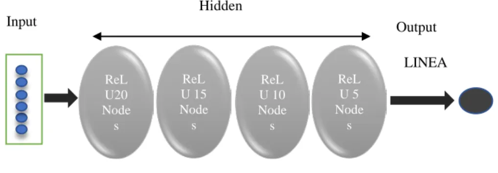
In this research, the number of neurons in a hidden layer was varied to observe the impact of the hidden layers on the neural network's performance. The results revealed that a Fully Connected Network made of 20×15×10×5 nodes with four hidden layers was optimal and therefore they were chosen to train the networks as illustrated in Figure 1.
This work uses a Fully Connected Network made of 20×15×10×5 nodes with four hidden layers, as illustrated in Figure 1. The input features of the network are standard gravity model variables such as
GDP, distance, border, colonial relationship, and trade agreement, to mention a few, as summarized in Table 1
below.
Source: Own work.
Figure 1. Fully connected feedforward artificial neural network
Panel data estimation approach
This study conducts a regression analysis with panel data PPML through econometric gravity model—described as the workhorse of international trade and one of the most successful empirical models in economics (Anderson & van Wincoop, 2003) and statistical software—Stata 15.1. Cross-sectional or pooled ordinary least squares (OLS) regression is often used to estimate the gravity trade model. Yet, biased results may be created by these estimation approaches (Cheng & Wall, 2005). This is because heterogeneity is not allowed in the error term for standard cross- sectional regression equations, thus yielding overestimated results. An advantage of using the panel data estimation method is that it can increase the
volume of informative data in variability with less collinearity among the variables (Leitão, 2010), which allows more degrees of freedom and efficiency.
Following Wohl & Kennedy (2018) and Gopinath et al.
(2021), in this study, the panel data from 1990 to 2017 is analyzed to estimate the regression coefficients with the PPML estimation of the gravity model. The econometric results from using the variables suggested by NNA indicate a high R-square for most parameters (Table A4). Most of the variables in the econometric model are statistically significant, and at the 0.01%
level, but similarities and differences are visible from the R-square. The out-of-sample forecast error of root mean squared error (RMSE) is computed and compared with that of the best ANN (see Table 4).
Table 1 Features
Variable name Representation Feature description 𝑙𝑙𝑎𝑎𝑋𝑋𝑖𝑖𝑖𝑖,𝑡𝑡 Exports from China to the World
(millions of US. dollars)
The logarithm of China’s bilateral exports to partner country at year t
𝑙𝑙𝑎𝑎𝐺𝐺𝐺𝐺𝐺𝐺 exporter GDP, Annual % The logarithm of GDP of China at year t
𝑙𝑙𝑎𝑎𝐺𝐺𝐺𝐺𝐺𝐺 importer GDP, Annual % The logarithm of GDP of partner country j at year t
𝑙𝑙𝑎𝑎 distance Bilateral distance The logarithm of the distance between China and partner country
𝐶𝐶𝐶𝐶𝑎𝑎𝐷𝐷𝑖𝑖𝐶𝐶 Contiguity 1 if the two trading partners share a border a common
border,0 otherwise
𝐶𝐶𝐶𝐶𝐶𝐶𝑙𝑙𝑎𝑎𝑎𝑎𝐶𝐶_off Common Language 1 if the two trading partners share a common official or
primary language, 0 otherwise
𝐶𝐶𝐶𝐶𝑙𝑙𝐶𝐶𝑎𝑎𝐶𝐶 Colonial relationship 1 if one of the trading partners for origin and destination
ever in a colonial relationship
𝑙𝑙𝑎𝑎𝑙𝑙𝑙𝑙𝑎𝑎𝑗𝑗𝐷𝐷 Infrastructure index The logarithm of the infrastructure of China
𝑙𝑙𝑎𝑎𝑙𝑙𝑙𝑙𝑎𝑎𝑖𝑖𝑡𝑡 Infrastructure Index The logarithm of the infrastructure of partner country j
at year t
𝑂𝑂𝑂𝑂𝑂𝑂𝑂𝑂 One Belt One Road, Dummy 1 if the origin country is a OBOR member
𝐴𝐴𝐴𝐴𝐴𝐴𝐴𝐴𝐴𝐴 Association of Southeast Asian
Nations, Dummy
1 if the origin country is an ASEAN member
𝐴𝐴𝐴𝐴𝐶𝐶 East African Community, Dummy 1 if the origin country is an EAC member
𝐴𝐴𝐴𝐴𝐺𝐺𝐶𝐶 Southern African Development
Community, Dummy
1 if the origin country is a SADC member ReL
U20 Node s
Input Output
Hidden
ReL U 15 Node s
ReL U 10 Node s
ReL U 5 Node s
LINEA
The output neuron can be computed as follow:
𝛼𝛼=𝑙𝑙 �� 𝑤𝑤𝑖𝑖 𝑥𝑥𝑖𝑖 𝑁𝑁 𝑖𝑖=0
� ( 3)
Where 𝑙𝑙 is the activation function, 𝑥𝑥𝑖𝑖 denoted the numerical input, and the weights are represented by 𝑤𝑤𝑖𝑖. There have been various activation functions that are applied in the context of ANNs. One commonly used activation function is the sigmoid function, which takes a value between 0 and 1 by applying a threshold.
However, we will be using the rectified linear unit
(ReLU) as the activation function. ReLU function refers to the type of activation function returning to the max (0, x). In the perspective of artificial neural networks, the rectifier or ReLU activation function (Brownlee, 2019) is an activation function denoted as the positive part of its argument:
𝑙𝑙(𝑥𝑥) =𝑥𝑥+= max (0,𝑥𝑥) (4)
Where 𝑥𝑥 is the input to a neuron. The rectified linear unit activations function is depicted in Figure 2.
Source: Own work.
Figure 2. Line plot of rectified linear activation for negative and positive inputs Over-fitting is a possible problem with ANN
models. In order to avoid it, cross-validation was applied, whereas the dataset was divided randomly into training observations (70 percent of the dataset) and testing observations (30 percent of the dataset). We applied the training dataset to develop the estimators, then fed the independent variables from the test dataset into those estimators to engender predicted trade values for the out-of-sample observations. The root-mean- square error (RMSE) is used to measure the accuracy of the out-of-sample prediction. RMSE values are computed as the square root of the average of squared errors between the predicted values and the actual values as seen from the Equation below:
𝑂𝑂𝑅𝑅𝐴𝐴𝐴𝐴=�1
𝑎𝑎 �(𝐶𝐶�𝑖𝑖− 𝐶𝐶𝑖𝑖)2
𝑛𝑛 𝑖𝑖=1
(5)
Where 𝐶𝐶�𝑖𝑖 is the predicted observation, 𝐶𝐶𝑖𝑖 is the actual observation considered equal to the model, and 𝑎𝑎 represents the number of observations or data sets for the study.
D ATA SOURCES AND METHODOLOGY
Dataset
The study uses the data, which covers a panel data set of 162 countries from 1990 to 2017. Therefore, our data set entails 4536 observations of bilateral export flows (162 × 161 country pairs). There are various sources of data that were applied for data analysis. UN- Comtrade database was used to obtain the data for bilateral trade (exports). At the same time, the World Development Indicators (WDI, 2018) database was utilized as a source for GDP (importer, exporter) in billions of current U.S. dollars. Data on location and dummies indicating contiguity (common border), common language (official language), and colony (colonial relationship) were taken from the Centre d’Etudes Prospectives et d’Informations Internationales (CEPII). The Bilateral Distance between China and its partners was taken from the CEPII distance database.
The Infrastructure index grounded in Carrere &
Grigoriou (2011), and Limao (2001) approach is computed by applying four variables proxying the transport infrastructure from the IRF world road statistics and WDI (W.B., 2018): total roads network, total paved roads, railway network, and the number of telephones mainline per person. The model was 0
2 4 6 8 10 12
-15 -10 -5 0 5 10 15
estimated using China’s bilateral exports between its new Silk Road partners. The summary of the 13 economic features that are used in the model is presented in Table 1 (Features). GDP and the amount of exports are reported in current U.S. $. Most of these features are commonly applied in Gravity Model and are all deemed well-defined, based on a solid background, and then suitable for this study.
Implementing these features for the prediction purpose allows us to compare our performance against the Gravity Model (i.e., our baseline model).
Cleaning Techniques and Features
To avoid deviations in data and potential obstacles in the prediction procedure, we had applied several data cleaning techniques before the analysis started.
First, we extrapolate the missing data using the preprocessing methods. Second, we removed incomplete data from the data set. That is, we did not work with data points that have missing feature values.
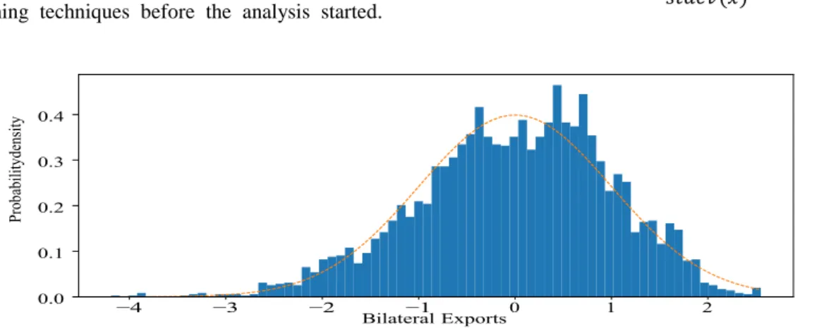
Third, we removed all trade flow values with no values, as they are not economically significant and cause outlier problems. Fourth, we took the log of data to achieve a smoother distribution of the data, as shown in Figure 3. At last, we removed data from 1990 to 1991 as our focus is to predict current trade flows. For the neural network, we standardize the continuous variables (exporter’s GDP, importer’s GDP), scaling them so that their means equal zero and their standard deviations equal one using Equation 6 below.
𝑋𝑋𝑆𝑆=𝑥𝑥𝑖𝑖− 𝐶𝐶𝑚𝑚𝑎𝑎𝑎𝑎(𝑥𝑥)
𝐷𝐷𝐷𝐷𝑎𝑎𝑚𝑚𝑠𝑠(𝑥𝑥) ( 6)
Source: Own work.
Figure 3. Histogram of feature space distribution of bilateral exports
A NALYSIS AND DISCUSSION
The gravity model is considered as the workhorse tool in examining international trade. It measures the relationship between the trading behavior of two countries based on their GDPs and distances. It offers accurate predictions of international trade and has solid theoretical foundations (Wohl & Kennedy, 2018). The outputs of gravity model estimations are compared to those of neural networks using the MSE (mean squared error) and RMSE (root mean squared error) together with other metrics that may be used. MSE is a squared RMSE, an absolute measure of fit, and is reported in the same unit as the response variable.
Table 2 shows the results of the evaluations. For the baseline dataset, the OLS estimator has an out-of- sample root mean squared error of $16.05 billion, the PPML estimator has an out-of-sample RMSE of $6.53 billion, and the neural network has an out-of-sample RMSE of $3.83 billion. For the dataset with country fixed effects, the OLS estimator has an out-of-sample RMSE of $11.30 billion, the PPML estimator has an out-of-sample RMSE of $9.79 billion, and the neural network has an out-of-sample RMSE of $1.91 billion.
For the dataset with country-year fixed effects, the
OLS estimator has an out-of-sample RMSE of $6.66 billion, the PPML has an out-of-sample RMSE of
$8.17 billion, and the neural network has an out-of- sample RMSE of $1.89 billion. These analyses were repeated several times, allowing for variation in the random training-test division and the neural network development, and these outcomes are representative.
For illustrating the forecasting application of our model, the neural network has been trained on the full dataset with country fixed from 1990 to 2012 and applied to predict bilateral trade export between China and its major trading partners in the Silk and Road Initiative.
The estimation covers the period from 2013 to 2017.
The neural network’s estimates seem reasonably close to the actual trade values to some extent, particularly around 2013 and 2015.
The accuracy of the network models is measured by RMSE (Chong, 2013; Gbongli et al., 2019), which is calculated as the difference between actual and predicted values of the dependent constructs, i.e., export in the present context. We provided the result of the neural network with the actual GDPs of China and its BRI partners, as seen from Figure 4 and Table 3.
The neural network’s estimations are reasonably close to actual trade values even five years beyond the training period.
Table 2
Trade predictions using estimators in respect to generated RMSE (In Millions of US $)
Models OLS PPML Neural Networks
Baseline Model $16.05 $6.53 $3.83
Country-fixed effects $11.30 $9.79 $0.1908
Country-year fixed effects
$6.66 $8.17 $1.89
Adjustment and architecture
Dependent variable:
𝑙𝑙𝑎𝑎(𝑋𝑋𝑖𝑖𝑖𝑖+ 1)
Dependent variable 𝑋𝑋𝑖𝑖𝑖𝑖,𝑡𝑡
Exports, distance, infrastructure, GDP, (𝐷𝐷𝐷𝐷𝑎𝑎𝑎𝑎𝑎𝑎𝑎𝑎𝑙𝑙𝑎𝑎𝑖𝑖𝑠𝑠𝑚𝑚𝑎𝑎 𝐶𝐶𝑚𝑚𝑎𝑎𝑎𝑎= 0)
(𝐴𝐴𝐷𝐷𝑎𝑎.𝐺𝐺𝑚𝑚𝑠𝑠. = 1) Source: Own work.
Table 3
Neural network predictions versus actual trade values (in Millions Us $)
Countries Predictions 2013 2014 2015 2016 2017
Kenya Actual
Predicted
6.5075 6.5595
6.6929 6.6094
6.7719 6.6306
6.7472 6.6550
6.7472 6.6911
Rwanda Actual
Predicted
5.1275 5.02705
5.0606 5.0700
5.0873 5.0933
5.0356 5.0966
5.0356 5.1489
Zimbabwe Actual
Predicted
5.6168 5.8410
5.6062 5.8689
5.7351 5.8860
5.5883 5.8881
5.5882 5.9284 Source: Own work.
Table 4 below presents a summary of the models’
performances. The table reports both the average RMSE values as well as the values of 𝑂𝑂2 . These values were used to predict the correctness of the Gravity and ANN models. The smaller the value of RMSE, the better the accurateness of the prediction. 𝑂𝑂2 ranges from 0 to 1: If 𝑂𝑂2= 0, the model always fails to predict the target variable, and if 𝑂𝑂2= 1 the model perfectly predicts the target variable. Any value between 0 and 1 signposts what percentage of the target variable, applying the model, can be elucidated by the features. If 𝑂𝑂2< 0 it reveals that the model is no better than one that continually predicts the mean of the target variable.
The traditional gravity model (OLS) output was used to compare those of neural networks to some extent. However, particular attention was put on the PPML (considered the more robust estimator to deal with the panel data and non-linearity data set) to compare with ANN outputs. From Table 4, the gravity model result is assessed against the ANN model in terms of RMSE and 𝑂𝑂2. The neural network with country-fixed effects has the most significant
predictive accuracy among the models. It attains a 98.05 percent reduction in out-of-sample RMSE compared to the PPML estimator on the same dataset and a 98.32 percent reduction compared to the OLS estimator.
Moreover, using the identical set of features as the Gravity model (baseline model) based on the OLS estimator, the ANN technique (baseline model) achieves a notable improvement of above 0.49 in the test set’s 𝑂𝑂2 score. Similarly, using the identical set of features as the Gravity model (baseline model) grounded in the PPML estimator, the ANN technique (baseline model) achieves a remarkable improvement of above 0.03 in the test set’s 𝑂𝑂2 score. This signifies that neural networks successfully discover non-linear interactions between features compared to the Gravity model, mainly with the OLS estimator, a purely linear model of logarithmic features. Using the same dataset, this result discloses that we were able to achieve higher predictive ability without calling into time series models, which was one of the purposes of the research work.
Source: Own work.
Figure 4. Neural network predictions compared to actual trade
C ONCLUDING REMARKS
The study aims to examine the macroeconomic effects of China’s BRI quantitatively. It remains essential to understand why trade happens the way it arises and to expand economic ties between countries, a theoretical question that can be facilitated through gravity models employing traditional specifications. Moreover, predicting trade between two countries (i.e., China and African countries with a high degree of accuracy is an essential and practical inquiry that neural networks can patronize. Using a gravity model and neural network technique and focusing more on the area of trade investment under the BRI, our quantitative exercises suggest critical potential advantages of the BRI to the economies.
Drawing upon the results of panel data regression and ANN, this research offers two insights. The first is that China’s bilateral export flow under the new Silk Road initiatives significantly positively affects the countries involved. This finding is important since its supports the concept that the BRI could bring trade opportunities to developing countries by improving their bilateral trade with China.
Second, our simulations have shown that using neural networks is a promising approach in predicting bilateral trade flow when making predictions with other economic variables of the same period. Neural network techniques are a sound methodology for making predictions about economic data. This paper compares the various estimation procedures of the gravity model – OLS and PPML– with the neural network. Employing the same set of features as the Gravity model (baseline model) based on the OLS estimator, the ANN technique (baseline model) achieves a notable improvement of above 0.49 in the test set’s 𝑂𝑂2score. In a similar vein with the same set of features as the Gravity model (baseline model) grounded in the PPML estimator, the ANN technique (baseline model) attains a remarkable improvement of above 0.03 in the test set’s 𝑂𝑂2score. The neural networks associated with fixed country effects showed a more accurate estimation than a baseline model even with country-year fixed effects. Regarding the OLS
estimator and Poisson Pseudo-Maximum Likelihood (PPML), however, they showed mixed results. It appears that the ANN estimation of the gravity equation was superior over the other procedures to enlighten the variability of the dependent variable (export) towards the prediction accuracy based on root mean squared error (RMSE) and R-square. The scope of the gap in predictive accuracy recommends that neural networks capture non-linear interactions of independent constructs that influence trade in ways not captured by OLS or PPML models. Therefore, the results stress that we were able to achieve higher predictive ability without calling into time series models, which was one of the purposes of the research work.
The implication drawn from findings for policymakers is that developing nations in East Africa could enhance exports performance by partaking in the BRI, which brings FDI to improve trade-supporting infrastructure and expand and upgrade local production capacity. Policy-makers, analysts, and businesses would all be able to profit by exact scales about China’s bilateral exports among its new Silk Road members. To entirely grasp the BRI’s potential, policymakers need to assess country-specific barriers for building links to global value chains, which could be high costs and key natural resources, lacking high- skill workforce, inefficient customs operations, outdated transport systems, inadequate information, and communication technology infrastructure, poor governance, and corruption, to mention few. Therefore, they require to formulate appropriate policies and measures to address the issues and work in close cooperation with other B&R nations and key stakeholders to co-create value for all as to searching for sustainable development.
One heading for future research is to use neural networks to anticipate the impacts of intra-regional trade or regional integration. Future research subjects could apply alternative artificial neural network structures such as radial basis function neural networks and recurrent neural networks instead of multilayer perceptron neural networks and use the output of the PPML model as inputs to artificial neural networks.
REFERENCES
ANDERSON, J. E. (1979). A Theoretical Foundation for the Gravity Equation. American Economic Review, 69(1), 106–116. https://doi.org/10.1126/science.151.3712.867-a
ANDERSON, J. E. & VAN WINCOOP, E. (2003). Gravity with Gravitas: A Solution to the Border Puzzle. American Economic Review, 93(1), 170–192. https://doi.org/10.1257/000282803321455214
ANDERSON, J. E. & VAN WINCOOP, E. (2003). Gravity with gravitas: A solution to the border puzzle. American Economic Review, 93(1), 170–192.
ATHEY, S. (2018). The Impact of Machine Learning on Economics. The Economics of Artificial Intelligence: An Agenda.
AZIZI, N., REZAKAZEMI, M. & ZAREI, M. M. (2019). An intelligent approach to predict gas compressibility factor using neural network model. Neural Computing and Applications, 31(1), 55–64. https://doi.org/10.1007/s00521- 017-2979-7
BAIER, S. L. & BERGSTRAND, J. H. (2009). Bonus vetus OLS: A simple method for approximating international
trade-cost effects using the gravity equation. Journal of International Economics, 77(1), 77–85.
https://doi.org/https://doi.org/10.1016/j.jinteco.2008.10.004
BAJARI, P., NEKIPELOV, D., RYAN, S. P. & YANG, M. (2015). Machine Learning Methods for Demand Estimation.
American Economic Review, 105(5), 481–485. https://doi.org/10.1257/aer.p20151021
BALDWIN, R. & TAGLIONI, D. (2006). Gravity for dummies and dummies for gravity equations.
BAXTER, M. (2017). Robust Determinants of Bilateral Trade. Society for Economic Dynamics., 591.
BERGSTRAND, J. H. (1989). The Generalized Gravity Equation, Monopolistic Competition, and the Factor- Proportions Theory in International Trade. Source: The Review of Economics and Statistics, 71(1), 143–153.
https://doi.org/10.2307/1928061
BOFFA, M. (2018). Trade Linkages Between the Belt and Road Economies (English). Policy Research Working Paper.
https://doi.org/10.1596/1813-9450-8423
BROWNLEE, J. (2019). A Gentle Introduction to the Rectified Linear Unit (ReLU). Machine Learning Mastery.
CARRERE, C. & GRIGORIOU, C. (2011). Landlockedness, Infrastructure and Trade: New Estimates for Central Asian Countries. ffhalshs-00556941.
CHAN, F. T. S. & CHONG, A. Y. L. (2012). A SEM–neural network approach for understanding determinants of interorganizational system standard adoption and performances. Decision Support Systems, 54(1), 621–630.
https://doi.org/10.1016/j.dss.2012.08.009
CHENG, I. & WALL, H. J. (2005). Controlling for Heterogeneity in Gravity Models of Trade and Integration. Federal Reserve Bank of St. Louis Review, 87(1), 49–64. https://doi.org/10.3886/ICPSR01313
CHINA’S TRADE WITH BRI COUNTRIES SURGES TO $1.34 TRILLION IN 2019. (2020). The Economic Times, 15 January 2020.
CHONG, A. Y. L. (2013). A two-staged SEM-neural network approach for understanding and predicting the determinants of m-commerce adoption. Expert Systems with Applications, 40(4), 1240–1247.
https://doi.org/10.1016/j.eswa.2012.08.067
CHUNG, C. (C. P. . (2018). What are the strategic and economic implications for South Asia of China’s Maritime Silk Road initiative? The Pacific Review, 31(3), 315–332. https://doi.org/10.1080/09512748.2017.1375000
DEARDORFF, A. V. (1998). Determinants of Bilateral Trade: Does Gravity Work in a Neoclassical World? NBER Working Paper No. W5377, January, 7–32. https://doi.org/10.3386/w5377
DENNIS, A. (2006). The Impact of Regional Trade Agreements and Trade Facilitation in the Middle East North Africa Region. In Policy Research Working Paper.
DONAUBAUER, J., GLAS, A., MEYER, B. & NUNNENKAMP, P. (2018). Disentangling the impact of infrastructure on trade using a new index of infrastructure. Review of World Economics, 154(4), 745–784.
DUMOR, K. & YAO, L. (2019). Estimating China’s Trade with Its Partner Countries within the Belt and Road Initiative Using Neural Network Analysis. Sustainability, 11(5), 1449. https://doi.org/10.3390/su11051449
EATON, J. & KORTUM, S. (2002). Technology, Geography, and Trade. Econometrica, 70(5), 1741–1779.
ELIF, N. (2014). Estimating And Forecasting Trade Flows By Panel Data Analysis And Neural Networks. Journal of the Faculty of Economics, 64(1), 85–111.
FEENSTRA, R. C. (2015). Advanced international trade: theory and evidence. Princeton university press.
FEENSTRA, R. C., MARKUSEN, J. R. & ROSE, A. K. (2001). Using the gravity equation to differentiate among alternative theories of trade. Canadian Journal of Economics/Revue Canadienne D`Economique, 34(2), 430–447.
FLINT, C. & ZHU, C. (2019). The geopolitics of connectivity, cooperation, and hegemonic competition: The Belt and Road Initiative. Geoforum, 99. https://doi.org/10.1016/j.geoforum.2018.12.008
GARSON, G. . (1991). Interpreting neural network connection weights. Artif. Intell. Expert, 6, 46–51.
GBONGLI, K. (2017). A two-staged SEM-AHP technique for understanding and prioritizing mobile financial services perspectives adoption. European Journal of Business and Management, 9(30), 107–120.
GBONGLI, K., XU, Y. & AMEDJONEKOU, K. M. (2019). Extended Technology Acceptance Model to Predict Mobile-Based Money Acceptance and Sustainability: A Multi-Analytical Structural Equation Modeling and Neural Network Approach. Sustainability, 11(13), 3639. https://doi.org/10.3390/su11133639
GBONGLI, K., XU, Y., AMEDJONEKOU, K. M. & KOVÁCS, L. (2020). Evaluation and Classification of Mobile Financial Services Sustainability Using Structural Equation Modeling and Multiple Criteria Decision-Making Methods. Sustainability, 12(4), 1288. https://doi.org/10.3390/su12041288
GOPINATH, M., BATARSEH, F. A., BECKMAN, J., KULKARNI, A. & JEONG, S. (2021). International agricultural trade forecasting using machine learning. Data \& Policy, 3.
GRADOJEVIC, N. & YANG, J. (2000). The Application of Artificial Neural Networks to Exchange Rate Forecasting:
The Role of Market Microstructure Variables. Bank of Canada.
HERRERO, A. G. & XU, J. (2017). China’s Belt and Road Initiative: Can Europe Expect Trade Gains? China \&
World Economy, 25(6), 84–99.
HOLSLAG, J. (2017). How China’s New Silk Road Threatens European Trade. The International Spectator, 52(1), 46–
60. https://doi.org/10.1080/03932729.2017.1261517
HUANG, Y. (2016). Understanding China’s Belt & Road Initiative: Motivation, framework and assessment. China
Economic Review. https://doi.org/10.1016/j.chieco.2016.07.007
HUSSAIN, Z., HANIF, N., SHAHEEN, W. A. & NADEEM, M. (2019). Empirical analysis of multiple infrastructural covariates: an application of gravity model on Asian economies. Asian Economic and Financial Review, 9(3), 299.
IWANOW, T. & KIRKPATRICK, C. (2009). Trade facilitation and manufactured exports: Is Africa different? World Development, 37(6), 1039–1050.
KHAN, M. K., SANDANO, I. A., PRATT, C. B. & FARID, T. (2018). China’s Belt and Road Initiative: A global model for an evolving approach to sustainable regional development. Sustainability (Switzerland), 10(11).
https://doi.org/10.3390/su10114234
KHASHEI, M., RAFIEI, F. M. & BIJARI, M. (2013). Hybrid Fuzzy Auto-Regressive Integrated Moving Average (FARIMAH) Model for Forecasting the Foreign Exchange Markets. International Journal of Computational Intelligence Systems, 6(5), 954–968. https://doi.org/10.1080/18756891.2013.809937
KIM, K. & MARIANO, P. (2020). Trade Impact of Reducing Time and Costs at Borders in the Central Asia Regional Economic Cooperation Region.
LEE, H. & ITAKURA, K. (2018). The welfare and sectoral adjustment effects of mega-regional trade agreements on ASEAN countries. Journal of Asian Economics, 55, 20–32. https://doi.org/10.1016/j.asieco.2017.09.001
LEITÃO, N. C. (2010). The gravity model and United States’ trade. European Journal of Economics, Finance and Administrative Sciences, 21, 92–100. http://www.scopus.com/inward/record.url?eid=2-s2.0- 77955031213&partnerID=40&md5=d5f6b4e2e21db6849172cb4624970d9a
LEUNG, M. T., CHEN, A.-S. & DAOUK, H. (2000). Forecasting exchange rates using general regression neural networks. Computers & Operations Research, 27(11–12), 1093–1110. https://doi.org/10.1016/S0305- 0548(99)00144-6
LI, B. & DUAN, Y. (2014). Trade facilitation assessment and its impact on China’s service trade exports: Based on transnational panel data empirical research (in Chinese). Int. Bus, 1, 5–13.
LIMAO, N. (2001). Infrastructure, Geographical Disadvantage, Transport Costs, and Trade. The World Bank Economic Review. https://doi.org/10.1093/wber/15.3.451
LISI, F. & SCHIAVO, R. A. (1999). A comparison between neural networks and chaotic models for exchange rate prediction. Computational Statistics & Data Analysis, 30(1), 87–102. https://doi.org/10.1016/S0167- 9473(98)00067-X
METULINI, R., PATUELLI, R. & GRIFFITH, D. A. (2018). A spatial-filtering zero-inflated approach to the estimation of the gravity model of trade. Econometrics, 6(1), 9.
MOÏSÉ, E. & SORESCU, S. (2013). Trade Facilitation Indicators. In OECD Trade Policy Papers no.144.
https://doi.org/10.1787/5k4bw6kg6ws2-en
NUMMELIN, T., HÄNNINEN, R. & OTHERS. (2016). Model for international trade of sawnwood using machine learning models. Natural Resources and Bioeconomy Studies, 74.
PIERMARTINI, R. & YOTOV, Y. (2016). Estimating Trade Policy Effects with Structural Gravity. 2016–10.
POUREBRAHIM, N., SULTANA, S., THILL, J. C. & MOHANTY, S. (2018). Enhancing trip distribution prediction with Twitter data: Comparison of neural network and gravity models. Proceedings of the 2nd ACM SIGSPATIAL International Workshop on AI for Geographic Knowledge Discovery, GeoAI 2018.
https://doi.org/10.1145/3281548.3281555
PÖYHÖNEN, P. (1963). A Tentative Model for the Volume of Trade between Countries. Weltwirtschaftliches Archiv, 90, 93–100.
RAVEN, J. (2001). Trade and Transport Facilitation : A Toolkit for Audit, Analysis, and Remedial Action.
RIPLEY, B. D. (1996). Pattern Recognition and Neural Networks. In Pattern Recognition and Neural Networks.
Cambridge University Press. https://doi.org/10.1017/CBO9780511812651
SALETTE, G. & TINBERGEN, J. (1965). Shaping the World Economy. Suggestions for an International Economic Policy. Revue Économique. https://doi.org/10.2307/3498790
SCOTT, J. E. & WALCZAK, S. (2009). Cognitive engagement with a multimedia ERP training tool: Assessing computer self-efficacy and technology acceptance. Information and Management, 46(4), 221–232.
https://doi.org/10.1016/j.im.2008.10.003
SHEELA, K. G. & DEEPA, S. N. (2013). Review on Methods to Fix Number of Hidden Neurons in Neural Networks.
Mathematical Problems in Engineering, 2013, 1–11. https://doi.org/10.1155/2013/425740
SILVA, J. M. C. S. & TENREYRO, S. (2006). The Log of Gravity. Review of Economics and Statistics, 88(4), 641–658.
https://doi.org/10.1162/rest.88.4.641
SILVA, J. M. C. S. & TENREYRO, S. (2011). Further simulation evidence on the performance of the Poisson pseudo- maximum likelihood estimator. Economics Letters, 112(2), 220–222.
SONIA CIRCLAEYS, C. K. & KUMAZAWA, D. (2017). Bilateral Trade Flow Prediction. Stanford Final Reports.
TINBERGEN, J. (1962). Shaping the world economy; suggestions for an international economic policy.
TKACZ, G., HU, S. & OTHERS. (1999). Forecasting GDP growth using artificial neural networks. Bank of Canada Ottawa.
VARIAN, H. R. (2014). Big Data: New Tricks for Econometrics. Journal of Economic Perspectives, 28(2), 3–28.
https://doi.org/10.1257/jep.28.2.3
WILSON, J. S., MANN, C. L. & OTSUKI, T. (2003). Trade Facilitation and Economic Development: A New Approach to Quantifying the Impact. The World Bank Economic Review, 17(3), 367–389.
https://doi.org/10.1093/wber/lhg027
WOHL, I. & KENNEDY, J. (2018). Neural Network Analysis of International Trade. Office of Industries. U.S.
International Trade Commission (USITC).
WU, B. (1995). Model-free forecasting for nonlinear time-series (with application to exchange rates). Computational Statistics & Data Analysis, 19(4), 433–459.
YOTOV, Y. V. (2012). A simple solution to the distance puzzle in international trade. Economics Letters, 117(3), 794–
798. https://doi.org/https://doi.org/10.1016/j.econlet.2012.08.032
YOTOV, Y. V, Piermartini, R., Monteiro, J.-A. & Larch, M. (2016). An advanced guide to trade policy analysis: The structural gravity model.
ZAKI, C. (2014). An empirical assessment of the trade facilitation initiative: econometric evidence and global economic effects. World Trade Review, 13(1), 103–130. https://doi.org/10.1017/S1474745613000256
ZHANG, G. P. (2003). Time series forecasting using a hybrid ARIMA and neural network model. Neurocomputing, 50, 159–175. https://doi.org/10.1016/S0925-2312(01)00702-0
ZHANG, Y. B. & LIU, J. (2016). Trade facilitation measurement of the “Silk Road Economic Belt” and China’s trade potential (in Chinese). Finance. Sci., 5, 112–122.
ZHU, J. B. & LU, J. (2015). Research and application of trade facilitation evaluation indicator system (in Chinese). J.
Hunan University, 6, 70–75.