A conceptual magnetic fabric development model for the Paks loess in Hungary
Bradák, B.a, Újvári, G.b,c, Seto, Y.d, Hyodo, M.a,d, Vígh, T.e
a Research Center for Inland Seas, Kobe University, Nada, Kobe 657-8501, Japan
b Institute for Geological and Geochemical Research, Research Centre for Astronomy and Earth Sciences, Hungarian Academy of Sciences, H-1112 Budapest, Hungary
c Center for Nuclear Technologies, Technical University of Denmark, DTU Risø Campus, Denmark d Department of Planetology, Kobe University, Nada, Kobe 657-8501, Japan
e Department of Physical Geography, Eötvös University, Budapest H-1117, Hungary
Abstract
We describe magnetic fabric and depositional environments of aeolian (loess) deposits from Paks, Hungary, and develop a novel, complex conceptual sedimentation model based on grain size and low-field magnetic susceptibility anisotropy data. A plot of shape factor (magnetic fabric parameter) and dry deposition velocity estimated from grain-size reveals primary and secondary depositional processes during the sedimentation of loess. Primary ones are driven by gravity, with poorly oriented MF for fine grain materials, and by tangential stress, with flow-aligned or flow-transverse fabric for coarser grain sediments. The fabric developed by a primary process is called depositional magnetic fabric. Secondary processes develop in unconsolidated sediments, beginning right after deposition and terminating before the start of diagenesis. Under slow sedimentation conditions, deposited materials are likely to be exposed near the surface for longer periods. Therefore, relatively strong winds with a stable direction can alter the fabric of non-buried surficial sediments. As a result, grain orientations may change from scattered, non-flow oriented fabric to flow-oriented fabric. This type of fabric, developed by a secondary process, is called transformed magnetic fabric, and is characterized by relatively well-defined grain orientation, which allows us to estimate a dominant wind direction.
Keywords: Anisotropy of magnetic susceptibility; magnetic fabric; Sedimentology, loess;
Pleistocene;
1. Introduction
Low field anisotropy of magnetic susceptibility (AMS) provides a useful tool to characterise magnetic fabric (MF) of materials. MF, characterized by AMS, reflects the alignment of magnetic contributors in the material, including high saturation magnetization minerals, which have preferred dimensional orientation (pdo) controlled magnetic
anisotropies (e.g. magnetite and maghemite) and other minerals with crystallographic preferred (crystallographic axis) orientation (cpo) controlled magnetic anisotropies (e.g.
paramagnetic minerals). Therefore, the MF can provide potential insight into various processes, including the type and orientation of material transport, flow energy, post- sedimentary processes, and stress fields (Tarling and Hrouda, 1993). AMS has been often applied to loess, loess-like sediments, and paleosols since the pioneering studies of Liu et al.
(1988). The MF of these sediments reflects various sedimentary and post-sedimentary environments.
Through the development of not flow-oriented (poorly lineated, mainly foliated) fabric, the gravitational force dominates over the tangential force. The not flow-oriented fabric displays quasi-horizontal foliation with a dip of a few degrees and scattered alignment of the elongated grains in a horizontal plane, without any characteristic fabric lineation. According to
Derbyshire et al. (1988), the fabric of the ‘typical’ (i.e. Aeolian) loess is isotropic. The poorly lineated, mainly foliated loess theory is supported by studies of Hus (2003) and Wang and Løvlie (2010). Hus (2003) observed that gravitational force and compaction play leading role
in developing the MF of loess. The original aim of the experiments of Wang and Løvlie’s (2010) was not the characterization of the AMS of loess, although they simulated the sedimentation of loess by dry deposition and wetting the deposited material. They also reported the magnetic fabric results (e.g. streoplot analysis) which shows the poorly lineated, mainly foliated MF (Wang and Løvlie, 2010; Figure 2, page 397).
Major characteristics of a flow-aligned fabric are that elongated grains tend to align in parallel with the transport direction and usually display an up-flow tilting (imbricated MF, a- axis imbrication. A 5–20° dip to the horizontal plane of foliation is indicated by the deviation of minimum magnetic suceptibility (kmin) from the vertical (e.g. Thistlewood and Sun, 1991).
The kmin deviation from vertical and its orientation was defined as a marker of imbrication of magnetic particles, and used to infer paleowind directions by Nawrocki et al. (2006).
The poorly or better clustered orientation of elongated grains, distributed along the
imbrication (foliation) plane defines current orientation (mainly deposition orientation). This MF type is the most common in loess deposits, and has widely been used for estimating paleowind directions (e.g. Begét et al., 1990; Thistlewood and Sun, 1991; Sun et al., 1995;
Wu et al., 1998; Lagroix and Banerjee, 2002, 2004a; Bradák, 2009; Liu and Sun, 2012; Ge et al., 2014; Peng et al., 2015; Xie et al., 2016). Various methods were developed to verify the orientation and wind-blown origin of the MF. Comparison of confidence ellipsoids and various AMS parameters were used to quantify the accuracy of maximum magnetic
susceptibility (kmax) orientations as indicators of paleowind directions (Lagroix and Banerjee, 2004b; Zhu et al. 2004; Zhang et al., 2010). Determination of the deviation of kmin inclination from vertical is also a commonly applied method to separate the fabric of undisturbed (wind- blown, less than 20°) and redeposited/reworked loess (e.g. Zhu et al., 2004). Theoretically if the dust is deposited on a nearly horizontal surface the orientation of a bedding dominated fabric will be defined by the minimum susceptibility axis (kmin), its orientation being the pole
to the bedding plane. The maximum and intermediate susceptibility axes (kmax and kint) will lie in the bedding plane. The primary axis defining the depositional plane is kmin.
Unfortunately, some essential criteria of this method include the statistically significant lineation of the fabric, which cannot be met in various cases (e.g. low energy transport during
‘dust falls’). Similarly, the pronounced deviation of kmin from vertical does not necessarily mean redeposition (e.g. imbrication).
In biaxial prolate orientation (shear stress related) / flow-transverse fabric (sedimentary process related) (AB plane imbricated fabric, pencil fabric), the a-axes of clasts are aligned perpendicularly to the flow direction, and the intermediate axes are aligned in the flow direction. Two different types of sedimentary flow-transverse fabrics are described in the literature: I.) in this fabric the orientations of principal susceptibilities are well separated, and current orientation is indicated by a 10–20° dip of the foliation plane (kmin) and the orientation of intermediate magnetic susceptibility (kint). II.) this type of stereoplot of flow-transverse fabric is characterized by well-clustered kmax directions and kmin and kint are intermixed along an axis on the foliation plane. The development of MF is interpreted as indicating strong currents, traction and rolling of grains during transportation and a stable condition after deposition (Tarling and Hrouda, 1993; Tauxe, 1998). In both types, the transport direction is perpendicular to the orientation of kmax. Similar fabrics are also reported from Alaskan loess and interpreted as the results of shear stress (Lagroix and Banerjee, 2004b) and reconstructed in the laboratory environment (Rees, 1983), but in general such flow-transverse fabrics are rare, especially in loess sediments (Lagroix and Banerjee, 2004b; Bradák et al., 2011; Bradák- Hayashi et al. , 2016; Zeeden et al., 2015).
New observations and interpretation of the loess MF suggest that surface processes (e.g.
permafrost, erosion by run-off water and redeposition), the paleogeomorphology (e.g. slope, local depressions) and pedogenic processes play more profound roles during dust deposition
and the post-depositional period than previously expected (e.g. Lagroix and Banerjee, 2004a;
Bradák et al., 2011; Bradák and Kovács, 2014; Ge et al., 2014; Taylor and Lagroix, 2015;
Bradák-Hayashi et al., 2016). Disturbed, altered and inverse fabrics are easily being developed under such conditions. If sedimentation takes place on a slope, the dip direction can be identified by the alignment of principal susceptibilities: the tilt of kmin directions from vertical and inclination of the plane defined by the intermixed kmax and kint from the horizontal plane (Rees 1966, 1971; Bradák et al., 2011; Ge et al., 2014). The deviation of kmin from vertical (‘slope deposition-like fabric’) was interpreted as resulting from a cryptic post- depositional deformation/reworking during permafrost processes (Lagroix and Banerjee 2004a; Taylor and Lagroix 2015) (Figure 1e). Biogenic activity may cause isotropic magnetic fabric through pedogenesis. However, Elwood (1984) found no difference between the
magnetic fabrics of non-bioturbated and bioturbated materials. By contrast, the deviation of kmin inclination from vertical, along with the chaotic alignment of the principal susceptibilities and isotropic magnetic fabric was observed in different paleosols (Hus 2003 and Matasova et al. 2001). As a possible indicator of bioturbation, inverse magnetic fabric was found in paleosols intercalated in loess layers in some studies (Matasova and Kazansky 2004; Bradák et al. 2011; Bradák-Hayashi et al., 2016). For an inverse fabric, the direction of kmax is perpendicular to the almost horizontal bedding plane (kmax inclination ~ 90°). The inverse fabric is caused by the vertical orientation of the grains (pdo) (Bradák-Hayashi et al., 2016).
The results of magnetic fabric measurements are supported by micromorphological studies, demonstrating the vertical orientation of grains in the fabric of paleosols. Originally the term was used to describe magnetic fabric with the same character driven by crystallographic anisotropy of siderite, or due to uniaxial single domain magnetite (Rochette, 1988).
Nevertheless, inverse fabric is rarely observed in loess sequences. Such a fabric was identified only one profile in paleosol horizons (Bradák et al. 2011; Bradák-Hayashi et al. 2016). The
'inverse fabric' indicates both the vertical alignment of minerals (pdo) due to vertical pedogenic processes and crystallographic anisotropy (cpo) of minerals such as fine-grained magnetite or siderite (Hrouda, 1982; Rochette, 1988; Márton et al., 2010).
Despite the clear relationship between transport/depositional direction and MF orientation revealed by extensive works on loess magnetic fabric and paleowind directions, only a few studies have attempted to improve our understanding of MF parameters related to transport velocity and energy (e.g. Zhang et al., 2010; Bradák and Kovács, 2014). No investigations have mentioned so far that MF changes may be due to changing transport/deposition energy.
This study aims at revealing the relationship between various transport/depositional energies and MF development, thereby describing the depositional environment during the formation of loess primary MF.
2. Materials and methods 2.1 Materials
The Paks loess profile is located north of the town Paks in the Pannonian Basin, Hungary, on the right bank of the Danube River. In the brickyard, a 16-m thick loess/palaeosol
sequence was cleaned and sampled (Figure 1). The sediments analysed in this study are yellow and yellowish-grey in colour, and consists of fine-grained, silty, or silty sand materials with a homogeneous matrix or occasionally poorly developed fine laminated structure. Based on their grain size distribution (GSD), the samples are classified into three groups: fine- grained loess (fL; GSD volumetric mean < 34 µm) dominated by silt components; medium- grained loess (mL; GSD volumetric mean 34-63 µm) with a larger amount of coarse silt; and coarse-grained loess/very fine sand (cL; GSD volumetric mean > 63 µm) with a significant fine sand component (e.g. sandy loess-type loess and aeolian very fine sand samples, 63 - 125
µm). The sedimentary characteristics of the samples collected are described in detail in Supplementary Material 1. Based on GSDs and sedimentary character (homogeneous structure and no sign of redeposition), all samples were identified as wind-blown in origin.
Indicators of redeposition such us poorly sorted materials, lenticular bedding and lamination containing clayey paleosol and silty loess laminae were not observed in the sampled layers.
The few identified laminas in the sequence are made up of the same materials consistent material with as those in the homogeneous part and the laminas may have developed due to temporary fluctuations of the transportation energy. Thus, these samples are considered as excellent material to identify possible MF changes due to variations in transportation energy.
Signs of bioturbation such as biogalleries and burrowing, and indicators of pedogenesis like ped structure or soil horizons were not observed in the sampled layers. This observation result cannot exclude possibility of ‘crypt post-depositional working’ (Lagroix and Banerjee, 2002, 2004a, b; Taylor and Lagroix, 2015). Despite the lack of any sign of redeposition, and/or pedogenesis, care must be taken for interpretations of MF due to possibility of ‘crypt post- depositional reworking’ (e.g. Lagroix and Banerjee 2002, 2004a, b; Taylor and Lagroix, 2015).
Oriented block samples of about 10×10×10 cm3 were collected every 10-cm depth interval in preliminary sampling. Cubic specimens of 2×2×2 cm3 were cut from the block samples. No plastic holder was applied to avoid fabric deformation during sampling and sample
preparation. The MF was investigated using 509 pieces of 2×2×2 cm3 cubic sample; in general 6–10 samples were collected from each 10 cm sediment interval. This sampling strategy enabled a high-resolution MF record to be obtained with statistically significant datasets for each studied horizon and layer.
2.2 Methods
Hysteresis measurements and stepwise isothermal remanent magnetisation (IRM) acquisition experiments were conducted using a Micromag 3900 alternating gradient magnetometer (Princeton Measurements Co.). IRMs were acquired in fields of up to 1,000 mT and measured quasi-continuously. Temperature variation in magnetic susceptibility, K(T), was measured using an MFK1-FA Kappabridge susceptibility meter coupled with a CS-4 furnace apparatus for high-temperature susceptibility measurements ‘in air’ (AGICO, Czech Republic).
MF orientations of 509 samples were determined by measuring a specimen in 15 positions using a KLY-3S Kappabridge (AGICO) instrument. Intensities and directions of principal susceptibilities (kmax, kint, kmin) were determined by computer analysis, and numerous statistical parameters were calculated and used to characterise the MF calculated using the principal susceptibility values (Anisoft 4.2 software). During data verification, results with negative F statistics (F < 3.48; 95% significance level; Jelinek 1977) were excluded. F12 (F12
> 5) and e12 were also examined (Lagroix and Banerjee, 2004a) along with the alignment of principal susceptibilities on stereoplots. Samples taken from the same 10 cm thick
stratigraphic horizons were analysed together on stereoplots. Lagroix and Banerjee (2004a) summarised the criteria for a fabric with a well-defined orientation (statistically significant kmax) for individual loess samples. An area of uncertainty around the orientation of principal axes is quantified by 95% confidence ellipses that have semi-axes, denoted herein by epsilon (ε). At the specimen level, the 95% confidence uncertainty ellipse of kmax is defined by semi- axes ε12 and ε13, where ε12 is the half-angle uncertainty of kmax in the plane joining kmax and kint, and ε13 is the half-angle uncertainty of kmax in the plane joining kmax and kmin. The
maximum allowable ε12 of statistical significance, indicating well-oriented grains in individual samples, is 22.58°. These criteria were used to determine primary loess with significant orientation (Lagroix and Banerjee 2004a). The F12 – ε12 plot was studied to
reveal significant lineation in the samples (Zhu et al., 2004). Furthermore, the relationship between foliation and F23 was also investigated (Zhu et al., 2004) in order to reveal well resolved magnetic foliation in the fabric (F23>10). The analyses include the investigation of F12 and bulk susceptibility relations to identify random measurements error in samples with low bulk susceptibility (Zhu et al., 2004). When the F12 and ε12 statistics did not show strong anisotropy, but the alignment of the principal susceptibilities, related to the same stratigraphic horizons, indicated some characteristic orientation or fabric in the stereoplots, the data of the samples were used (Supplementary Material 1 and 2). The data of samples with low F12, high ε12 and isotropic alignment of the principal susceptibilities were excluded from the analysis. Finally, data of 180 samples were removed. We used mean values of the
samples’ AMS parameters taken from the same 10 cm thick stratigraphic horizon (‘Hpa’
sample groups; Figure 1c; Supplementary Material 1). Both the significance ellipsoid and average group statistics were calculated by Anisoft 4.2 software.
Basic AMS parameters, such as foliation (F), lineation (L) and corrected degree of anisotropy (Pj) were calculated, as defined by Stacey et al. (1960)
F = kint/kmin
where kint is the intermediate low field susceptibility and kmin is the minimum low field susceptibility, Balsey and Buddington (1960)
L = kmax/kint
where kmax is maximum low field susceptibility and kint is intermediate low field susceptibility, and Jelinek (1981)
P = exp √{2[(ηmax− ηm)2+ (ηint− ηm)2 + (ηmin− ηm)2] }
where ηmax = lnkmax; ηint = lnkint; ηmin = lnkmin and
η𝑚 = √η3 𝑚𝑎𝑥 × η𝑖𝑛𝑡 × η𝑚𝑖𝑛.
Relationship between the shape of the susceptibility ellipsoid (T) and the degree of anisotropy (P), was characterised by Jelinek diagrams (Jelinek, 1981). The T value indicates the
dominance of oblate or prolate shapes in MF, and was calculated according to Jelinek (1981).
Thus, this diagram possibly allows for distinguishing various transport facies by exploiting the influence of transport/deposition energy on the alignment of magnetic grains.
T = (2 × ηint - ηmax - ηmin) / (ηmax - ηmin)
where ηmax = lnkmax; ηint = lnkint; ηmin = lnkmin.
The dominant influence of F or L on MF, was assessed using Flinn diagrams (Flinn, 1962).
Originally, the Flinn diagram was applied to describe the shapes of strain ellipsoids. In MF studies, a susceptibility ellipsoid can be characterised by the F and L parameters and plotted on Flinn diagram (Tauxe, 2010). Dominance of F indicates an oblate ellipsoid, which is characteristic for calm, stable sedimentary environments. By contrast, the dominance of L indicates a prolate ellipsoid, indicating sediment transport by higher velocity currents. The objective of using the Flinn diagram is that the F and L parameters can be analysed along with the shape of the susceptibility ellipsoid.
The characterisation of stresses and transport energy during fabric production was done by q- β diagrams (Taira, 1989), where q determines the shape factor introduced by Granar (1958)
q = (kmax – kint)/[0.5 × (kmax + kint) – kmin]
where kmax, kint, kmin are the maximum, intermediate and minimum low field susceptibilities, and β stands for the inclination of minimum principal susceptibility, respectively. The factor q corresponds to the intensity of magnetic lineation in the magnetic foliation plane with the intensity of foliation. In this case, the angle of imbrication is defined by the tilt of the short axis (Taira, 1989). The q–β diagram was applied by Taira (1989) to reveal the link between the imbrication angle and the shape factor. The q and β values are considered to be related to gravitational and tangential stresses in fabric production (Taira, 1989). Separated fields are defined on the diagram using specific β and q values of sediment materials transported in different modes, deposited in different environments, and characterised by diverse sedimentary structures. Note, however, that care must be taken during the application of Taira-diagram, as samples from various environments and settings (aeolian and water-lain sediments) were used to define its fields. Nevertheless, the main tendencies in transportation energy change can be well recognized on these plots.
The alignments of principal susceptibilities (kmax: maximum magnetic susceptibility; kint: intermediate magnetic susceptibility; kmin: minimum magnetic susceptibility) were plotted on stereonets, using equal-area nets and a geographical coordinate system.
In this study, GSD was measured using a Beckman Coulter LS 13320 laser diffraction particle size analyser. Before the analyses, samples were treated with 7 ml of 1% ammonium hydroxide, then put into a rotator and allowed to rotate for a minimum of 12 hours. The
German standard DIN 4022 (EN ISO 14688, international standard) for soil/rock
classification was applied during grain size measurements. Grain size classes were given as defined by Konert and Vandenberghe (1997)
For predicting dry deposition, resistance models are widely used (Seinfeld and Pandis, 2006). In such models the effects of sub-processes like turbulent diffusion, gravitational settling and surface collection are represented with corresponding resistances, the inverse of deposition velocity (Zhang et al., 2001; Seinfeld and Pandis, 2006). In this work, Dry
deposition velocity (DDV) was calculated using the mean grain size of loess sediments, based on the parametrisation of Zhang et al. (2001) for grass vegetation (reference height = 0.2 m, neutral atmosphere):
DDV = 𝑣𝑡+ 1 𝑟𝑎+ 𝑟𝑠
where vt is the fall or terminal velocity, ra and rs are aerodynamic and surface resistances.
This type of vegetation is the most characteristic of the loess steppe; other types are not considered to simplify our model. As an input for the Zhang model, fall/terminal velocity was calculated following Ferguson and Church (2004), with parameters C1 = 18 and C2 = 1 for quartz grains (density = 2.65 g cm-3). For further details on the Zhang model and related calculations, see Zhang et al. (2001) and/or Újvári et al. (2016).
The well-polished samples were studied using a JEOL JSM-6480LAII scanning electron microscope (SEM) equipped with an energy dispersive X-ray spectroscope (EDS). To obtain flat and smooth surfaces, samples were impregnated with a low-viscous resin (Petropoxy 154) and polished byabrasives of SiC and Al2O3 without lubricant (to prevent alteration of clay minerals) in advance. For SEM observations, we used back-scattered electron imaging.
Chemical analyses using the EDS were obtained at 15 kV and 0.4 nA. Data corrections were made by the ZAF method with well-established natural/synthesized materials as chemical
standards. The X-ray elemental maps were acquired on the SEM EDX operated at 15 kV and 1 nA.
4. Results
4.1 Rock magnetism
Throughout the various rock magnetic experiments, pilot specimens of loess with different grain sizes behaved quite similarly.
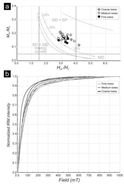
The ratio of remanent coercive force to coercive force (Hcr/Hc) ranges from 2.8 to 4.2, and that of saturation remanence to saturation magnetisation (Mrs/Ms) varies between 0.11 and 0.21. The Day plot indicates that all types of loess settles to an area of single domain + multi- domain (SD + MD) magnetic mineral character, with ca. 60–80% MD, showing a slight offset towards the superparamagnetic (SP) field (Figure 2a).
There are no characteristic differences in the IRM saturation of various loess types. The IRMs are ca. 80% saturated at 150 mT, and do not reach a complete saturation even at 300 mT (Figure 2b). The result suggests all of the samples are dominated by soft coercivity magnetic minerals, with a slight inclusion of high coercivity components.
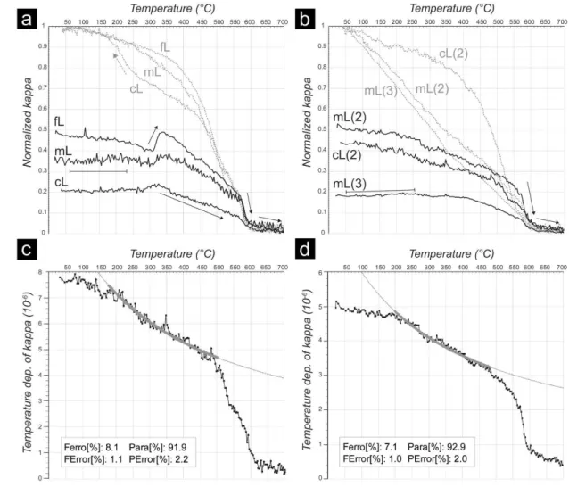
The typical thermal change in magnetic susceptibility (k) is shown in Figure 3a. The heating curves of k display a drop around 300°C, followed by an increase between 320 and 350°C. Above that, they show a linear decrease until about 570°C, having a sharp drop at 580°C, the Curie temperature of magnetite, followed by a gradual decrease to zero at about 680°C, the Curie temperature of hematite. Combined with the IRM acquisition experiment results, we infer that the soft components are carried by magnetite and maghemite, and a hard component is hematite, like those contributing to paleomagnetism of Chinese loess-paleosols (e.g. Yang et al., 2008, 2010). The slight decrease of k at about 300°C is due to thermal
decomposition of maghemite, and the increase between 320 and 350°C suggests neoformation of magnetite (Liu et al., 2010). The further heating brought thermal conversion of newly- formed magnetite into hematite. The linear decrease curve of k between 350 and 570°C reflects the thermal conversion (Deng et al., 2000; Liu et al., 2005). Some samples showing k- T curves with no increase in k around 300°C probably contain few maghemite grains, and thus they show convex decreasing curve between 350 and 570°C (Figure 3b). The recovered k much higher than the original k is possibly related to the neoformation of magnetite (or
maghemite) from clay minerals during the heating treatment (e.g. Ao et al., 2009).
4.2 Magnetic fabric parameter characteristics
The significance of lineation and foliation of individual specimens was tested and
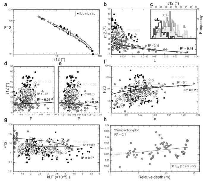
characterized by numerous ways (Figure 4). The ε12 – F12 plot reveals significant lineation
for cL. By contrast, weak or non-lineated fabric are observed for mL and fL sediments (Figure 4a). The diagram indicates the lineation becomes weaker as the grain size decreases, and ε12 values have large variability being different among three loess types; the most scattered (fL), least scattered (cL), and intermediate (mL) (Figure 4b, c). The all data L – ε12 plot indicates moderate inverse relationship (exponential trend, R2: 0.32), while the L – ε12 plots with only fL/mL data show no such relationship ( R2: 0.03/0.16, respectively) (Figure 4). A moderate correlation is observed for the plot with only cL data (R2: 0.44). There are no significant relationships among F, Pj, and ε12 (Figure 4d, e). Most of the samples from fL, mL and cL groups are characterised by F23>10 values in the F – F23 plot (Figure 4f). No significant relationship is observed between the bulk susceptibility and F12 (Figure 4g).
To reveal a possible influence of compaction in the MF, we examined vertical changes of F (Figure 4h). They show weak relationship (R2: 0.1), with a slight increase with depth.
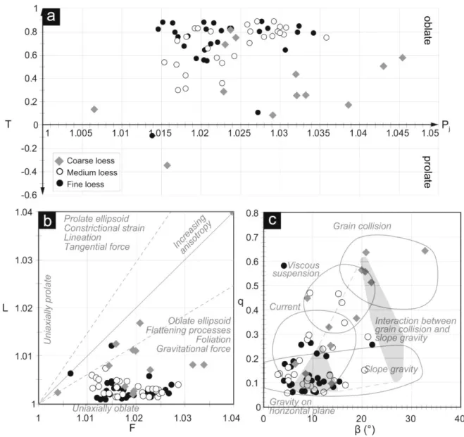
The T and Pj values on the Jelinek diagram show most samples have MF characterised by oblate T (disk-shaped) (Figure 5a). The data for the three sediment types are
undistinguishable on the diagram. The scattered cL data indicate prolate, triaxial, and oblate ellipsoid shapes (TcL: –0.35 to +0.88), with various degrees of anisotropy (including the most anisotropic samples; PcL: 1.006 to 1.045). Compared with mL and cL, fine loess samples exhibite less scatter, more than half of which are characterised by strongly oblate ellipsoids (TfL: > 0.8; average: 0.70) (Figure 5a).
Most samples display foliated fabric on the Flinn diagram (Figure 4b). The F values for the three loess groups are similar (fLavg: 1.018; mLavg: 1.019; mLavg: 1.020). In contrast to the F values, the L values are different. The MF of cL is more lineated (lineation cLavg: 1.008), compared to the MFs of fL (lineation fLavg: 1.003) and mL (lineation mLavg: 1.003) (Figure 4b).
The q–β diagram compares grain alignments to the sedimentary characters/environments (Taira,1998) (Figure 4c). The diagram indicates that gravity and currents dominate the deposition of fL and mL, whereas currents, viscous suspension, and grain collision dominate the deposition of cL. The fL and mL sediment types revealed similar average imbrication angles (βfL,mL: ~10.3° and 10.5). More scattered and higher maximum imbrication angles (average βcL: ~ 19°; βmax: 52.7°) are observed in the cL samples. In addition to changing imbrication angles, an increase in q is also evident in the cL samples, which reveals some weak points of the q–β diagram and the interpretation of β. Compared to the imbricated MF of some fL and mL samples, the MF of some sediments (e.g. 1-17, 5-15, 5-16, 5-18, 5-12, 5-20, 5-14) is possibly developed by different sedimentary processes. High β can be identified e.g.
in flow-transverse (biaxial prolate orientation) samples, which is developed by higher energy transport processes.
The principal susceptibilities in loess samples showed horizontally aligned fabrics (Supplementary Material 2); the scattered kmax directions aligned along the horizontal foliation (bedding) plane, and kmin formed a tight group around the bedding pole. In some loess samples, less scattered alignments were observed in kmax and kint, and deviation of kmin
from the vertical indicated a-axis imbrication and flow-aligned MF (Supplementary Material 2).
Well-aligned kmax andkint directions were observed in the fabrics of medium- and coarse- grained loess samples (Supplementary Material 2). Disturbance of the fabric, a-axis or flow- transverse MF (e.g. 1-17; 5-18) were identified by the scattered alignment and higher deviation from the vertical in the kmin of some sand layers.
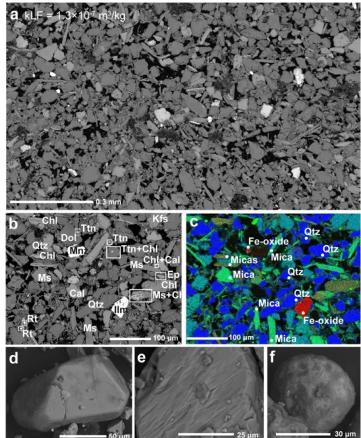
4.5 Scanning Electron Microscope observations
Scanning electron microscope (SEM) observations of loess samples demonstrate the appearance of various magnetic mineral components. The general overview of the material shows coarse grain, silt dominant microfabric, with few matrix (clay) appaerance between grains (Figure 6a). Along with the presence of minerals with higher iron content (magnetite, titanomagnetite, ilmenite), large amount of micas (e.g. muscovite) and chlorites were
observed in loess. Other common mineral components were quartz and calcite in relatively larger amounts. Apatite, rutile, K-feldspar and epidote were also observed (Figure 6b, c). The characteristic grain size of the grains present are between ~10 – 60 μm (Figure 6a, b, c).
During the morphological study of individual grains from sediments clear crystallographic planes (shape) could be recognized, along with some possible morphological marks of aeolian transport such as concave depressions, polished surfaces and rounded edges of grains (e.g.
Banak et al., 2013; Galović, 2016) (Figure 6d, e, f).
4.4 Grain size and DDV results
The GSDs of the studied sediments were mainly dominated by silt-size (5.5–63 μm) fractions, with a maximum proportion of 76.3% and median of 67%. Clay and fine sand fractions were present in similar proportions, and the clay and fine sand together are exceeding 40% in some samples (Supplementary Material 1). The mean grain size ranged between 26 (fine silt) and 161 μm (very fine/fine sand), mainly between 30–48 μm
(lower/upper quartiles; fine/coarse silt). Calculated DDVs ranged between 0.15 and 1.62 m sec-1, mostly between 0.18 and 0.26 m sec-1, depending on the sediment type. As the
sediments were dominated by silt and sand particles, gravitational settling was the main dry deposition mechanism. Particle deposition on vegetation (here, grass) is mainly driven by impaction for sizes between 3–5 and 50 μm, and by gravitational settling for > 50 μm particles.
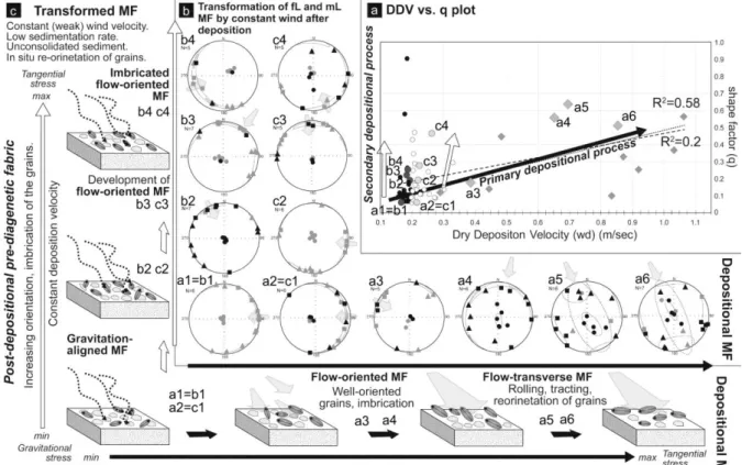
The DDV – q plot was found to be a useful tool for revealing various relationships between deposition velocity and the shape factor reconstructed from MF (Figure 7a). Strong positive relationship was expected assuming a possible link between grain alignment and increasing depositional velocity. It is presumed that higher depositional velocity aligns more grains in the main direction of deposition (wind), implying stronger lineation, higher degree of anisotropy and q in the MF. By contrast, only a weak relationship (R2: 0.2) was found between the two parameters (Figure 7a, black arrow). The decreasing influence of qfL and qmL on the relationship was notified due to the scatter in qfL and qmL, related to a narrow range of DDV. In other words, different degree of MF development (tangential stress) was identified in very similar depositional environments (Figure 7a; open arrows). To filter the dataset, samples with q>0.2 were removed from the regression calculations. The q=0.2 value indicates a boundary between calm, gravity-dominated and current-dominated environments in Taira diagram (Figure 5c). After filtering, the expected ‘ideal’ correlation (R2: 0.58) was
indeed found between DDV and q. Besides the identified primary tendency (increasing DDV along with increasing q) in the filtered fL and mL group, the lack of relationship between increasing q and constant DDV suggests the likely existence of a secondary process during sedimentation, before the diagenesis of dust (Figure 7a; open arrow).
5. Discussion and summary
The results of hysteresis measurements, IRM acquisition experiments, thermal change in k and SEM observations reveal that MF of the studied sediments are carried by ferro- and paramagnetic minerals. The ferromagnetic components are mainly magnetite
(titanomagnetite) and maghemite, with slight amounts of hematite. The Day plot shows the presence of ferromagnetic components with a mixed MD (ca. 70%) and SD (ca. 30%) character (Figure 3a). We cannot exclude the possibility of an influence of paramagnetic contributors to the susceptibility signal of samples characterised by magnetic susceptibility (k
< 5 × 10⁻⁴ SI; e.g. Hrouda and Jelinek, 1990). High amounts of paramagnetic contributors (ca.
90%) compared to ferromagnetic components is estimated by fitting a hyperbola offset along the y-axis of high-temperature k–T curves (Hrouda et al., 1997) (Figure 3c, d). On the
contrary, ~30-40% of soft ferromagnetic (<200 mT saturation) and ~60-70% of ‘harder’
component (>200 mT; e.g. hematite and paramagnetic components) were estimated by the analysis of hysteresis results. In summary, possible contributors to magnetic susceptibility include magnetite (titanomagnetite), maghemite, and paramagnetic grains such as muscovite, biotite and chlorite. The presence and possible influence of paramagnetic components is also supported by the SEM analysis, which indicates a high ratio of paramagnetic components (e.g. muscovite and chlorite) (Figure 6a). The overall match between grain size observed by SEM (including ferro- and paramagnetic grains) and laser-diffraction-based GSDs suggests
that the magnetic fabric of the studied materials is built up by coarser grain components.
Thus, possible relationships between DDV and AMS parameters can provide relevant information about the fabric development. Preservation of the crystallographic shape and aeolian features on the surface of some minerals indicate that strong chemical weathering did not happen after deposition (Figure 6c, d, e). The lack of thick, compact fine grain, clayey matrix between grains (along with the preserved features suggested above) excludes pedogenic origin of the fabric (Figure 6a).
The MFs of the sediment samples are characterised by foliated (Figure 4), strongly and horizontally oriented, oblate susceptibility ellipsoids (T > approximately 0.6; Figure 5a) and relatively scattered kmax distributions along the horizontal bedding plane on stereoplots (Supplementary Material 2; e.g. 1-1, 2-12, 5-8, 6-7). The foliated MF (Figure 4a, b; Figure 5b) and relation of q–β values (q < approximately 0.1; β < approximately 10°) suggest weak transportation currents and gravity-dominated particle deposition (Figure 5c). Clearly, the MF of the studied loess sediments was typical for aeolian loess deposits, as described in previous studies (e.g. Bradák and Kovács, 2014; Bradák-Hayashi et al., 2016, and references therein).
Compaction, indicated by increasing F with relative depth in the profile, also has minor influence on the MF of sediments (Supplementary Material 1, Diagram sheet). The increasing lineation of medium and coarse loess samples (Figure 4; Figure 5) demonstrates improved alignment of magnetic grains in the direction of transportation (e.g. Bradák and Kovács, 2014), likely due to higher-energy transportation processes. The increasing energy of transportation, also indicated by the q–β values (q > approximately 0.1; β > approximately 10°), implies higher-energy transportation via imbrication and grain to grain interactions (Figure 5b, c; e.g. Taira, 1998). In the case of flow-transverse fabric (Supplementary Material 2), the long axes of clasts are aligned perpendicularly to the flow direction. This alignment is
developed by rolling and tracting of particles during high-velocity transportation (e.g. Bradák and Kovács, 2014; Zeeden et al., 2015).
The relationships between DDV and q/L (Figure 7a, b) denote a ‘primary’ depositional process (Figure 7a,b; ‘black arrow’; a1 - a6 stereoplots) between reduced deposition velocities characteristic for fine-grained loess (with gravitation-aligned fabric) and the change of
gravitation-aligned fabric to flow-oriented and flow-transverse fabrics, due to increased deposition velocities for particles in coarser loess samples (Figure 7b, a1 – a6; Table 1). The suggested primary depositional process shows that the deposition of fine-grained loess (dust) is weakly influenced by tangential forces, dominantly by gravity or weaker winds. During the deposition of medium and coarse loess, the wind velocity increases and tangential force dominates the sedimentary processes. MF of fine loess, according to the primary processes, is non- or weakly oriented; it cannot be used to unambiguously determine a clear direction of deposition. Particle alignments are steadily improving with increasing transport energy; thus, the transport (wind) direction can be more clearly inferred from the primary MF of medium or coarse loess. To separate the suggested primary sedimentary processes, the use of the term
‘depositional MF’ is recommended. Along the tangential force, the crystallographic
anisotropy of various materials may influence the MF of loess. Some samples yielded very low kLF. Some observations (Rochette, 1987; Hrouda and Jelinek, 1990) suggest that MF of materials with low susceptibilities (kLFavg<5×10⁻⁴SI) can be influenced by paramagnetic components. Numerous samples are characterized by strongly oblate MF (Figure 5a;
Supplementary Material 2, ‘Diagrams’ sheet), which may also be the result of paramagnetic components, such as biotite and muscovite (Martín-Hernández and Hirt, 2003). The
crystallographic anisotropy of phyllosilicates is capable of weakening the anisotropy of the MF: the well aligned kmin directions are (subparallel to the crystallographic c-axis and)
perpendicular to the depositional plane. Compared to kmin, the kmax and kint axes are randomly
or poorly aligned (Biedermann et al., 2014). The thermal experiments (see above) also
support the appearance of paramagnetic components. Based on the evidences above we argue that the influence of paramagnetic components cannot unambiguously be excluded during the investigation of loess MF.
Besides the primary ‘depositional MF’ (increasing DDV and q), ‘secondary’ depositional process is also observed (Figure 7 a, b; ‘open arrow’; b1 - b4, c1-c4 stereoplots). For fL and mL samples, increasing q values are not associated with an increase in DDV (Figure 5a).
Beyond the limit of changes in q, variation in MF parameters such as L, β, and the alignment of principal susceptibilities (Figure 7b) are also recognised. This demonstrates well aligned principal susceptibilities and imbrication of grains by increasing q (Figure 5b). The
appearance of this phenomenon, along with MF variation, implies a complex development of MF.
The MF of the studied loess samples reveals complex fabric development. Based on the results obtained, we propose the following conceptual model to describe MF development (Figure 7c; Table 1). MF development during deposition is determined by the primary process(es) (Figures 7a, b, c). The deposition of fine sediments, such as fine loess, is mainly driven by gravity and weak currents, and for fine loess no clear fabric orientation can be detected (Figure 7; a1=b1 and a2=c2 samples; Table 1). By contrast, the sedimentation of coarse loess is influenced to a larger extent by higher velocity deposition, and thus the MF is imbricated and well-oriented (Table 1). Zhang et al. (2010) observed the lack of imbricated fabric in loess, and suggests the importance of precipitation (rain) in MF development during the summer monsoon period in China. During the summer monsoon period, the rain ‘helps to settle the sedimentary and magnetic grains’ (Zhang et al., 2010), and this process develop quasi-horizontal, non-imbricated fabric. In contrast to Chinese loess, previous studies on European loess suggested the disturbance of magnetic fabric during humid (interglacial)
periods. Processes acting in the vertical direction, such as the infiltrating water, are able to cause the quasi-vertical orientation of the grains (e.g. Bradák et al., 2011; Bradák-Hayashi et al., 2016; Taylor and Lagroix, 2015). To avoid such influence of various ‘interglacial or interstadial related’ processes (e.g. pedogenesis, increasing precipitation, strong water infiltration, erosion), our study is focussed on the aeolian sedimentation and diagenesis (see Material and Methods chapter, sample descriptions and this chapter below). The primary phase of loess sedimentation determines the MF character, when sedimentation rates and/or diagenesis are rapid, and able to preserve the original, so-called ‘depositional MF’.
‘Secondary’ depositional processes in sedimentation (here, post-sedimentary but pre- diagenetic processes; the reorientation of grains before diagenesis; not pedogenic processes or redeposition of the material after diagenesis) (Table 1) have an effect on MF when
sedimentation rate is low, diagenesis is slow, and MF exposed on the surface for a longer period. Winds of relatively constant direction and velocity are able to alter the MF of surficial deposits that are not being buried by addition of sediments leading to fast accretion. Grain orientations may gradually change from gravitation-aligned fabric to flow-oriented, imbricated fabric (Figure 7b; b1-b4; c1-c4). The shape parameter q = ~0.2 and some AMS parameters, summarized in Table 1 seemed to be marker values between the not flow-oriented primary depositional MF and transformed MF of fL and mL. To separate the MF developed by primary and secondary sedimentary processes, we suggest using the term ‘transformed MF’ for pre-diagenetically transformed fabric (described above). It must be noted, however, that the development of ‘transformed’ fabric does not imply redeposition, but rather in situ reorientation of the unconsolidated sediment (Fig. 7c). The described process, before the diagenesis of loess, yields an opportunity for determination of a dominant wind direction even after primary deposition of dust. In other words, the AMS can be rearranged by weak winds in
fine and medium-grained loess deposited and useful for the determination of paleowind direction.
The proposed model identifies some important and novel factors influencing the MF development of various aeolian sediments: the MF of sediments records the deposition velocity and direction, provided that both sedimentation and diagenesis are fast. Conversely, when the sedimentation rate is low and diagenesis is slow, ‘depositional MF’ is affected by other factors as well, and MF may change to ‘transformed MF’, having new MF characters including orientation parameters (i.e. paleowind direction).
Our proposed model implies that ‘depositional MF’ is strongly influenced by the transport/deposition velocity. Additionally, the secondary, in situ, post-depositional orientation, formed by the predominant regional wind regime, is responsible for the orientation of the ‘transformed MF’ of fine-grained sediments, such as loess. When MF exhibits a clear orientation, such as for loess deposits from the Chinese Loess Plateau (Liu and Sun, 2012; Ge et al., 2014; Peng et al., 2015) and Alaska (Lagroix and Banerjee, 2004), the pattern of the regional/local wind regime is relatively constant, as during the Pleistocene.
For loess from the European Loess Belt, however, the orientation of the MF and the
reconstructed wind directions are more scattered. For instance, the reconstructed glacial wind directions in Late Pleistocene from Kesselt section are NW (Hus, 2003), while from the Nussloch section (Antoine et al., 2009) NW and NE directions were inferred. However, care must be exercised during the interpretation of Nussloch results due to possible fabric
disturbance (Taylor and Lagroix, 2015). NW and SE paleowind directions were reconstructed from the Krems-Wachtberg section (Zeeden et al. 2015) and N-NE directions were revealed from the Late Pleistocene sections in Poland and Ukraine (Nawrocki et al. 2006). The shortly described scattered orientation is possibly due to the frequent change in the prevailing wind
directions over time and to the complexity of the wind regime in East Central Europe in that period.
Acknowledgments
We thank … … (…) for grain size measurements. A fellowship was awarded to … … at
… by the … . Part of this study was conducted within the cooperative research program of the
… . Research conducted by … … was supported by the … Scientific Research Fund … … .
References
Ao, H., Dekkers, M. J., Deng, C., Zhu, R. 2009. Palaeclimatic significance of the Xiantai fluvio-lacustrine sequence in the Nihewan Basin (North China), based on rock magnetic properties and clay mineralogy. Geophys. J. Int. 177, 913–924 doi: 10.1111/j.1365- 246X.2008.04082.x
Balsey, J.R., Buddington, A.F. 1960. Magnetic susceptibility anisotropy and fabric of some Adirondack granites and orthogneisses, American Journal of Science (Bradley volume), 258- A, 6–20.
Banak, A., Pavelić, D., Kovačić, M., Mandic, O., 2013. Sedimentary characteristics and source of loess in Baranja (Eastern Croatia), Aeolian Research 11, 129–139.
Begét, J. E., Stone, B. D., Hawkins, B. D. 1990.Paleoclimatic forcing of magnetic susceptibility variations in Alaskan loess during the late Quaternary. Geology 18, 40-43.
Biedermann, A. R., a, Koch, C. B., Lorenz W. E. A., Hirt, A. M. 2014. Low-temperature magnetic anisotropy in micas and chlorite. Tectonophysics 629, 63–74.
Bradák B. 2009. Application of anisotropy of magnetic susceptibility (AMS) for the determination of paleo-wind directions during the accumulation period of Bag Tephra, Hungary. Quaternary International 198, 77–84.
Bradák, B., Kovács, J., 2014. Quaternary surface processes indicated by the magnetic fabric of undisturbed, reworked and fine-layered loess in Hungary. Quaternary International 319, 76–87.
Bradák, B., Thamó-Bozsó, E., Kovács, J., Márton, E., Csillag, G., Horváth, E., 2011.
Characteristics of Pleistocene climate cycles identified in Cérna Valley loess–paleosol section (Vértesacsa, Hungary). Quaternary International, 234, 86–97.
Bradák-Hayashi, B., Biró, T., Horváth, E., Végh, T., Csillag, G. 2016. New aspects of the interpretation of the loess magnetic fabric, Cérna Valley succession, Hungary, Quaternary Research 86, 348–358.
Deng, C.L., Zhu, R.X., Verosub, K.L., Singer, M.J., Yuan, B., 2000. Paleoclimatic
significance of the temperature-dependent susceptibility of Holocene loess along a NW–SE transect in the Chinese loess plateau. Geophysical Research Letters 27, 3715–3718.
Derbyshire, E., Billard, A., Vliet-Lanoe, B.V., Lautridou, J.-P., Cremaschi, M., 1988. Loess and paleoenvironment some results of a European joint programme of research, Journal of Quaternary Science 3, 147-169.
Dunlop, D.J. 2002. Theory and application of the Day plot (Mrs/Ms versus Hcr/Hc) 2.
Application to data for rocks, sediments, and soils. Journal of Geophysical Research 107, 2057, 10.1029/2001JB000487.
Ellwood, B. B. 1984. Bioturbation: minimal effect on magnetic fabric of some natural and experimental sediments. Earth and Planetary Science Letters, 67, 367-376.
Ferguson, R.I., Church, M., 2004. A simple universal equation for grain settling velocity.
Journal of Sedimentary Research 74, 933–937.
Flinn, D., 1962. On folding during three-dimensional progressive deformation, Quarterly Journal of the Geological Society of London, 118, 385–433.
Galović, L., 2016. Sedimentological and mineralogical characteristics of the Pleistocene lo- ess/paleosol sections in the Eastern Croatia. Aeolian Research 20, 7–23.
Ge, J., Guo, Z., Zhao, D., Zhang, Y., Wang, T., Yi, L., Deng, C. 2014. Spatial variations in paleowind direction during the last glacial period in north China reconstructed from variations in the anisotropy of magnetic susceptibility of loess deposits. Tectonophysics 629, 353–361.
Granar, L. 1958. Magnetic measurements on Swedish varved sediments. Arkiv Geofysik 3, 1–
40. In: Hrouda, F. 1982. Magnetic anisotropy of rock and its application in geology and geophysics. Geophysical Survey 5, 37–82.
Haase, D., Fink, J., Haase, G., Ruske, R., Pécsi, M., Richter, H., Altermann, M., Jäger, K.-D.
2007. Loess in Europe—its spatial distribution based on a European loess map, scale 1:2,500,000. Quaternary Science Reviews 26, 1301–1312.
Horváth, E., Bradák, B. 2014. Sárga föld, lősz, lösz: short historical overview of loess research and lithostratigraphy in Hungary, Quaternary International 319, 1–10.
Hrouda, F., 1982. Magnetic anisotropy of rock and its application in geology and geophysics.
Geophysical Survey 5, 37-82.
Hrouda, F., Jelinek, V. 1990. Resolution of ferromagnetic and paramagnetic anisotropies in rock, using combined low-field and high-field measurements. Geophysical Journal
International 103, 75–84.
Hrouda, F., Jelinek, V., Zapletal, K. 1997. Refined technique for susceptibility resolution into ferromagnetic and paramagnetic components bases on susceptibility temperature-variations measurement, Geophysical Journal International 129, 715–719.
Hus, J.J. 2003. The magnetic fabric of some loess/paleosol deposits. Physics and Chemistry of the Earth 28, 689–699.
Jelinek, V. 1981. Characterization of magnetic fabric of rocks. Tectonophysics 79, 63–67.
Jordanova, N., Jordanova, D., Karloukovski, V. 1996. Magnetic fabric of Bulgarian loess sediments derived by using various sampling techniques. Studia Geophysica et Geodetica 40, 36–49.
Konert, M., Vandenberghe, J. 1997. Comparison of laser grain size analysis with pipette and sieve analysis: a solution for the underestimation of the clay fraction. Sedimentology 44, 523- 535.
Lagroix, F., Banerjee, S. K., 2002.Paleowind direction from the magnetic fabric of loess profile in central Alaska. Earth and Planetary Science Letters 195, 99-102.
Lagroix, F., Banerjee, S. K., 2004a. The regional and temporal significance of primary aeolian magnetic fabrics preserved in Alaskan loess. Earth and Planetary Science Letters 225, 379- 395.
Lagroix, F., Banerjee, S. K., 2004b. Cryptic post-depositional reworking in aeolian sediments revealed by the anisotropy of magnetic susceptibility. Earth and Planetary Science Letters 224, 453-459.
Lattard, D., Engelmann, R., Kontny, A., Sauerzapf, U. 2006. Curie temperatures of synthetic titanomagnetites in the Fe-Ti-O system: effects of composition, crystal chemistry, and thermomagnetic methods, Journal of Geophysical Research 111, B12S28,
doi:10.1029/2006JB004591.
Liu, Q., Deng, C., Yu, Y., Torrent, J., Jackson, M.J., Banerjee, S.K., Zhu. R. 2005.
Temperature dependence of magnetic susceptibility in an argon environment: implications for pedogenesis of Chinese loess/palaeosols. Geophysical Journal International 161, 102–112, doi: 10.1111/j.1365-246X.2005.02564.x.
Liu, X., Xu, T., Liu, T. 1988. The Chinese loess in Xifeng, II. A study of anisotropy of magnetic susceptibility of loess from Xifeng. Geophysical Journal 92, 349–353.
Liu, X. M., Shaw, J., Jiang, J. Z., Bloemendal, J., Hesse, P., Rolph, T., Mao, X. G. 2010.
Analysis on variety and characteristics of maghemite. Sci China Earth Sci, 2010, 53: 1–6, doi:
10.1007/s11430-010-0030-2.
Liu, W., Sun, J. 2012. High-resolution anisotropy of magnetic susceptibility record in the central Chinese Loess Plateau and its paleoenvironment implications. Science China, Earth Sciences 55, 488–494.
Martín-Hernández, F., Hirt, A. M., 2003. The anisotropy of magnetic susceptibility in biotite, muscovite and chlorite single crystals, Tectonophysics 367, 13– 28.
Matasova, G., Kazansky, A.Y. 2004. Magnetic properties and magnetic fabrics of Pleistocene loess/palaeosol deposits along west-central Siberian transect and their palaeoclimatic
implications. Geological Society, London, Special Publications 238, 145–173.
Matasova, G., Petrovský, E., Jordanova, N., Zykina, V., Kapička, A. 2001. Magnetic study of Late Pleistocene loess /palaeosol sections from Siberia: palaeoenvironmental implications Geophysical Journal International 147, 367–380.
Márton, E., Bradák, B., Rauch-Włodarska, M., Tokarski, A. K. 2010. Magnetic anisotropy of clayey and silty members of Tertiary flysch from the Silesian and Skole Nappes (Outher Carpathians). Stud. Geophys. Geod., 54, 121-134.
Nawrocki, J., Polechońska, O., Boguckij, A., Łanczont, M. 2006. Palaeowind directions recorded in the youngest loess in Poland and western Ukraine as derived from anisotropy of magnetic susceptibility measurements. Boreas 35, 266–271.
Peng, S., Ge. J., Li. C., Liu, Z., Qi., L., Tan, Y., Cheng, Y., Deng, C., Qiao, Y. 2015.
Pronounced changes in atmospheric circulation and dust source area during the mid- Pleistocene as indicated by the Caotan loess-soil sequence in North China. Quaternary International 372, 97–107.
Rees, A. I., 1966. The effect of depositional slopes on the anisotropy of magnetic susceptibility of laboratory deposited sands. Journal of Geology 74, 856-867.
Rees, A. I., 1971. The magnetic fabric of sedimentary rock deposited on slope. Journal of Sedimentary Petrology J 41/1, 307-309.
Rees, A.I. 1983. Experiments on the production of traverse grain alignment in a sheared dispersion. Sedimentology 30, 437–448.
Rochette, P., 1987. Magnetic susceptibility of the rock matrix related to the magnetic fabric studies. Journal of Structural Geology 9, 1015-1020.
Rochette, P., 1988. Inverse magnetic fabric in carbonate-bearing rocks. Earth and Planetary Science Letters 90, 229-237.
Seinfeld, J.H., Pandis, S., 2006. Atmospheric Chemistry and Physics: From Air Pollution to Climate Change. second ed. Wiley, New York.
Stacey, F.D., Joplin, G., Lindsay, J. 1960. Magnetic anisotropy and fabric of some foliated rock from S.E. Australia. Geophysica Pura Appl. 47, 30-40.
Sun, J. M., Ding, Z. L., Liu, T. S., 1995. Primary application of magnetic fabric mensuration of loess and paleosols for reconstruction of winter monsoon direction. Chinese Science Bulletin 40/21, 1976-1978 (in Chinese) in: Tang, Y., Jia, J., Xia, X. 2003. Record of
properties in Quaternary loess and its paleoclimatic significance: a brief review. Quaternary International 108, 33-50.
Taira, A. 1989. Magnetic fabrics and depositional processes. In: Taira, A. and Masuda, F.
(eds.) Sedimentary Facies in the Active Plate Margin, Terra Scientific Publishing Company.
Tokyo. 43–77.
Tarling, D.H., Hrouda, F. 1993. The magnetic anisotropy of rocks, Chapman and Hall, London, Glasgow, New York, Tokyo, Melbourne, Madras, 218.
Tauxe, L., 1998: Paleomagnetic principles and practice, KluwerAcademicPublishers, Dordrecht, Boston, London, 299 p.
Tauxe, L. 2010. Essentials of paleomagnetism. Berkeley: University of California Press, 489 p.
Taylor, S.N., Lagroix, F. 2015. Magnetic anisotropy reveals the depositional and post- depositional history of a loess-paleosol sequence at Nussloch (Germany): AMS of Nussloch loess-paleosol sequence, Journal of Geophysical Research, Solid Earth, 120, doi:10.1002.
Thistlewood, L., Sun, J. A., 1991.Paleomagnetic and mineral magnetic study of loess sequence at Liujiapo, Xi’an, China. Journal of Quaternary Science 6, 13-26
Újvári, G., Varga, A., Raucsik, B., János Kovács, J. 2014. The Paks loess-paleosol sequence:
a record of chemical weathering and provenance for the last 800 ka in the mid-Carpathian Basin, Quaternary International 319, 22–37.
Újvári, G., Kok, J.F., Varga, Gy., Kovács, J., 2016. The physics of wind-blown loess:
Implications for grain size proxy interpretations in Quaternary paleoclimate studies. Earth- Science Reviews 154, 247-278.
Wang,R, Løvlie, R. 2010. Subaerial and subaqueous deposition of loess: Experimental assessment of detrital remanent magnetization in Chinese loess. Earth and Planetary Science Letters 298, 394–404.
Wu, H. B., Chen, F. H., Wang, J. M., 1998. A study on the relationship between magnetic anisotropy of modern eolian sediments and wind direction. Chinese Journal of Geophysics (ACTA GeophysicaSinica) 41, 811-817 (in Chinese) in: Tang, Y., Jia, J., Xia, X., 2003.
Record of properties in Quaternary loess and its paleoclimatic significance: a brief review.
Quaternary International 108, 33-50.
Xie, X., Xian, F., Wu, Z., Kong, X., Chang, Q., 2016. Asian Monsoon variation over the late Neogeneeearly Quaternary recorded by Anisotropy of Magnetic Susceptibility (AMS) from Chinese loess. Quaternary International 399, 183-189.
Yang, T. S., Hyodo, M., Yang, Z. Y. Ding, ,L., Li, H. D., Fu, J. L., Wang, S. B., Wang, H.
W., Mishima, T., 2008. Latest Olduvai short‐lived reversal episodes recorded in Chinese
loess, Journal of Geophysical Research, 113, B05103, doi:10.1029/2007JB005264.
Yang T S, Hyodo M, Yang Z Y, Li, H., Maeda, M. 2010. Multiple rapid polarity swings during the Matuyama-Brunhes transition from two high-resolution loess-paleosol records.
Journal of Geophysical Research, 115: B05101, doi: 10.1029/2009JB006301.
Zeeden, C., Hambach, U., Händel, M. 2015. Loess magnetic fabric of the Krems-Wachtberg archaeological site, Quaternary International 372, 188–194.
Zhang, L., Gong, S., Padro, J., Barrie, L., 2001. A size-segregated particle dry deposition scheme for an atmospheric aerosol module. Atmospheric Environment 35, 549–560.
Zhang, R., Kravchinsky, V. A., Zhu, R., Leping, Y., 2010. Paleomonsoon route reconstruction along a W-E transect in the Chinese Loess Plateau using the anisotropy of magnetic susceptibility: Summer monsoon model. Earth and Planetary Science Letters 299, 436-446.
Zhu, R., Liu, Q., Jackson, M.J. 2004. Paleoenvironmental significance of the magnetic fabric of Chinese loess-paleosols since the last interglacial (< 130 ka). Earth and Planetary Science Letters 221, 55–69
Figures
Figure 1. The locality of Paks profile in Hungary (a) and in the European Loess Belt (b) (the European loess map is based on Haase et al., 2007). The stratigraphical position of the sampled fine, medium and coarse loess layers in the studied part of the succession between the Mende Base and Paks Double 2 paleosol horizons (for more information about the recent chronostratigraphical subdivision of the site please see Horváth and Bradák, 2014 and Újvári et al., 2014). The grey colour polygons indicate the distribution of loess in figure a and b. The numbers indicate the sampled horizons and sample groups summarized in Supplementary Material 1.
Figure 2. Results of rock magnetic experiments. (a) Day plot of hysteresis parameters.
Multi-domain (MD), single domain (SD), and superparamagnetic (SP) areas after Dunlop (2002). (b) Isothermal remanent magnetisation (IRM) acquisition curves of pilot samples.
Figure 3. Temperature variation in magnetic susceptibility (k–T plot). (a) ‘Complex’
heating curve. (b) ‘Simple’ heating curve. Offset hyperbola fit along the y-axis in the high temperature k–T curves of cL (c) and mL (d) pilot samples (e.g. Hrouda and Jelinek, 1990).
Black curve indicates heating; grey curve with dotted line indicates cooling. L, SL, and S denote loess, sandy loess, and sand, respectively.
Figure 4 Data verification and characterization of the foliation and lineation in the MF by (a) ε12 – F12 plot, (b) L – ε12 plot, (c) histogram of ε12, (d) F – ε12, (e) P – ε12, (f) F – F23, and (g) kLF – F12 plots, and (h) the relative depth – F ‘compaction’ diagram.
Figure 5. Plots of horizon mean magnetic fabric (MF) parameters. (a) Jelinek diagram (Jelinek, 1981). (b) Flinn diagram (after Flinn, 1962). (c) Taira diagram with separate areas related to various transportation and sedimentary environments and the characteristic aeolian parameters (grey areas) (after Taira, 1989).
Figure 6. Dispersion and alignment of the (magnetic) mineral components in the fabric of sediments (a, b, c). In the color figure (c) blue indicates quartz, red denotes mineral with high Fe content (e.g. magnetite) and green indicates minerals with lower Fe content (e.g. chlorite).
The crystalographic shape of ilmenite (d) reveal no strong weathering, the polished surface of muscovite (e) exhibits marks of wind errosion and the rounded shape and surface marks of magnetite (f) also indicates wind transport. Abbreviations are the following: Ap – apatite, Cal – calcite, Chl – chlorite, Dol – dolomite, Ep – epidote, Hem – hematite, Ilm – ilmenite, Ms – muscovite, Kfs – potassium feldspar, Ky – kyanite, Qtz – quartz, Rt – rutile, Ttn – titanite.
Figure 7. The primary (black arrow) and secondary (open arrow) processes revealed by the relationship between the (a) dry deposition velocity (DDV) and q anisotropy of magnetic susceptibility (AMS) parameter. Black circle: fine loess; white circle: medium loess; grey:
coarse loess. The black and white arrows indicate the observed two processes: black arrow – the increasing tangential stress during deposition by the increasing wind speed; open arrow – increasing tangential stress in samples at constant wind speed. The change of MF in both cases is described by the alignment of principal susceptibilities on stereoplots (b). The principal susceptibilities were plotted on stereoplots using an equal-area projection and geographical coordinate system. ■–maximum susceptibility, ▲–intermediate susceptibility,
●–minimum susceptibility; confidence angles for ≥ 5 data points are also plotted. All q values represent averages of samples originating from the same horizon of the section (we sampled every 10 cm of the studied sediment layers). Based on the characteristic change of the
alignment of principal susceptibilities on stereoplots a conceptual model for the development of loess was built (c). The ‘grains’ with arrows indicates the grains with preferred dimensional
orientation (pdo) such as magnetite and the grey polygons indicate paramagnetic components (e.g. phyllosilicates) which possibly can bias and weaken the pdo MF of the high saturation magnetization mineral components by their crystallographic preferred orientation (pdo).
Table 1. The comparison of depositional- and transformed magnetic fabric.
Supplementary materials
Supplementary Material 1. The AMS parameters of all measured sample and the sedimentological characterisation of the sampled horizons and the results of the grain size/AMS study. fL: loess; mL: medium loess; cL: coarse loess. Numbers on the sample/horizon indicate the sample size used to determine the AMS parameters of the discrete, 10-cm thick horizon.
Supplementary Material 2. The MF of the studied units. Each stereoplot represents the MF of a 10 cm thick sedimentary unit, defined by the results of individual sample
measurements (equal-area projection, geographical coordinate system, ■–maximum susceptibility, ▲–intermediate susceptibility, ●–minimum susceptibility).