five main phases of landscape
degradation revealed by a dynamic mesoscale model analysing
the splitting, shrinking, and
disappearing of habitat patches
Ádám Kun 1,2,3,4,5, Beáta oborny3,6 & Ulf Dieckmann1,7
the ecological consequences of habitat loss and fragmentation have been intensively studied on a broad, landscape-wide scale, but have less been investigated on the finer scale of individual habitat patches, especially when considering dynamic turnovers in the habitability of sites. We study changes to individual patches from the perspective of the inhabitant organisms requiring a minimum area for survival. With patches given by contiguous assemblages of discrete habitat sites, the removal of a single site necessarily causes one of the following three elementary local events in the affected patch: splitting into two or more pieces, shrinkage without splitting, or complete disappearance. We investigate the probabilities of these events and the effective size of the habitat removed by them from the population’s living area as the habitat landscape gradually transitions from pristine to totally destroyed.
On this basis, we report the following findings. First, we distinguish four transitions delimiting five main phases of landscape degradation: (1) when there is only a little habitat loss, the most frequent event is the shrinkage of the spanning patch; (2) with more habitat loss, splitting becomes significant;
(3) splitting peaks; (4) the remaining patches shrink; and (5) finally, they gradually disappear. Second, organisms that require large patches are especially sensitive to phase 3. This phase emerges at a value of habitat loss that is well above the percolation threshold. Third, the effective habitat loss caused by the removal of a single habitat site can be several times higher than the actual habitat loss. for organisms requiring only small patches, this amplification of losses is highest during phase 4 of the landscape degradation, whereas for organisms requiring large patches, it peaks during phase 3.
In today’s world, habitat fragmentation is a mostly anthropogenic process that threatens whole ecosystems1–5. Mitigating the consequences of, or altogether avoiding, habitat fragmentation is one of the main focuses of con- servation ecology6–9. Theoretical landscape ecology can aid such conservation efforts10 by supplying reliable measures of habitat fragmentation11,12 and by analysing models of population and metapopulations to predict the consequences of habitat fragmentation13–18. In particular, neutral landscape models (NLMs)19,20 have been introduced to provide a standard to which real landscape patterns can be compared.
The simplest NLM is the percolation map20 (Fig. 1). In a percolation map, habitat sites and non-habitat sites are randomly distributed according to the fraction p of habitat sites, with q = 1 − p denoting the fraction of
1Evolution and Ecology Program, International Institute of Applied System Analysis, Schlossplatz 1, A-2361, Laxenburg, Austria. 2Parmenides Center for the Conceptual Foundations of Science, Parmenides Foundation, Kirchplatz 1, D-82049, Pullach, Germany. 3Department of Plant Systematics, Ecology and Theoretical Biology, Loránd Eötvös University, Pázmány Péter sétány 1/C, H-1117, Budapest, Hungary. 4MTA-ELTE Theoretical Biology and Evolutionary Ecology Research Group, Pázmány Péter sétány 1/C, H-1117, Budapest, Hungary. 5Evolutionary Systems Research Group, MTA Centre for Ecological Research, Klebelsberg Kuno u. 3., H-8237, Tihany, Hungary.
6GINOP Sustainable Ecosystems Group, MTA Centre for Ecological Research, Klebelsberg Kuno u. 3., H-8237, Tihany, Hungary. 7Department of Evolutionary Studies of Biosystems, The Graduate University for Advanced Studies (Sokendai), Hayama, Kanagawa, 240-0193, Japan. Correspondence and requests for materials should be addressed to Á.K. (email: kunadam@elte.hu)
Received: 13 August 2018 Accepted: 17 July 2019 Published: xx xx xxxx
open
non-habitat sites. Such models are being extensively studied by physicists, within the field of percolation the- ory21. Percolation theory shows that in an infinite landscape of randomly distributed habitat and non-habitat sites (physicists sometimes refer to these as open and closed sites, respectively), an infinite cluster (also known as giant component or spanning patch) of habitat sites exists above a critical fraction pc of habitat sites, called the percola- tion threshold, whereas below that fraction no such cluster exists. Consequently, the probability that a randomly chosen habitat site belongs to the infinite cluster is zero below the percolation threshold and positive above it.
The threshold-like transition from connected to fragmented landscapes observed in percolation maps is instilling caution regarding the dangers of such drastic transitions occurring also in real landscapes20,22,23.
In recent years, NLMs have proliferated, becoming more and more sophisticated (for a review of landscape-generating algorithms, see24). For example, percolation maps have been generalized to incorporate more than two landscape-cover types13,25 or a gradient across which p varies from one end of the landscape to the other26–28. Also, as real landscapes generally show aggregated patterns, aggregation has been introduced to NLMs. For example, Gustafson and Parker29 randomly placed rectilinear clumps with random edge lengths onto a grid to create an aggregated pattern. Hiebler30 proposed an iterative method to produce landscapes with given pair-correlation probabilities (see also31). In hierarchical random landscapes32, the probability of assign- ing a patch to one of two landscape-cover types is first applied at larger spatial scales before being applied to the remaining habitat at smaller spatial scales, an approach that can be generalized to multiple landscape-cover types33,34. Realistically looking mosaic landscapes can also be generated by tessellation methods35,36, by fractal methods37–40, or by modifying/distorting existing landscape patterns to modify their spatial characteristics41. Many of the aforementioned methods are implemented in a readily available software package42. Finally, NLMs have been extended to three dimensions, to model soil layers or forest canopies43.
The spatially explicit modelling of ecological processes44,45 has become the focus of many ecological studies46. In the past three decades, an increasing number of population models have incorporated environmental heter- ogeneity15,25,30,31,39,47–58: the resultant body of literature has underscored how NLMs can aid the development of increasingly insightful and realistic landscape models. Compared to NLMs, landscape patterns or patch struc- tures used in experiments are usually simpler, such as a chessboard mosaic of resource-rich and resource-poor patches59–61 or patterns based on percolation maps62–64. To apply the insights derived from such simple experi- mental settings to more complex landscapes, suitable models are required, as experimental settings with more complex landscapes65,66 are rare.
An important development in NLM approaches has been the incorporation of temporal fluctuations into models23,49,52,53,67–73 and experiments74. In particular, Hagen-Zanker and Lajoie69 have proposed a neutral model
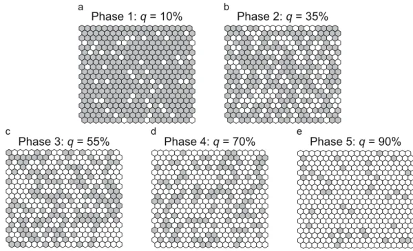
Phase 1: q = 10% Phase 2: q = 35%
Phase 3: q = 55% Phase 4: q = 70% Phase 5: q = 90%
c d e
b a
Figure 1. Levels of habitat loss and their differential consequences for habitat patches. Habitat sites (grey hexagons) and non-habitat sites (white hexagons) are distributed randomly on a hexagonal lattice. The shown levels of habitat loss q illustrate the five main phases of habitat degradation identified in this study (Table 1):
the percentages indicated above the panels are mid-interval values characteristic of Phases 1–5. For example, q = 10% means that 10% of habitat cover is lost and that 90% of habitat cover remains, which is the mid-interval value characteristic of Phase 1 (Table 1). The upper two panels show connected landscapes (Phases 1–2, where the level of habitat loss is below the percolation threshold, q < qc), while the lower three panels show fragmented landscapes (Phases 3–5, where q > qc). The pictures illustrate relatively small lattices (20 × 20 sites). In contrast, all numerical investigations in this study were carried out on larger lattices (100 × 100 sites), and a landscape’s property of being connected or fragmented is defined in the theoretical limit of infinite lattice size.
of landscape change, introducing a novel method for generating a landscape with multiple landscape-cover types and aggregation. Dynamic neutral landscape models (DNLMs), in general, eschew pre-defined spatial and tem- poral structures, to study the emergence of these structures from interactions among the components.
The DNLM we employ in the present study can arguably be considered as a minimalistic DNLM, because the process for changing the landscape is very simple and does not induce any spatial or temporal correlations among the habitability of the sites. Consequently, the habitat sites, initially being distributed randomly (as in NLMs), persist being free from any spatial or temporal correlations.
Even this simple representation of a dynamic landscape of habitable sites produces non-trivial emergent phe- nomena. Many interesting features have already been revealed before, especially by percolation theory elucidating the size distribution of habitable patches (percolation clusters) and the global connectivity of such patches (see23 for a review). In general, percolation theory has focused on global features, applying at the scale of the whole landscape, while assuming a static landscape. Here, we extend this view to dynamic landscapes and to the finer scale of individual patches.
This mesoscale is intermediate between the global scale (of the landscape as a whole) and the local scale (of individual habitat sites). From the perspective of an organism inhabiting the landscape, this intermediate scale of habitable patches is particularly important. When non-habitat sites are difficult to traverse for such an organism, it may be confined to a single patch for its whole life (concrete examples concerning plants are discussed by57).
Thus, any event changing the size of the patch the organism is inhabiting is crucial for the organism.
Important elementary events on the patch scale have been reviewed before, by Forman75 (pp. 407), Jaeger76, Akçakaya77, and Didham et al.78. Here we adopt this event-based view and develop it through a quantitative analysis of the events. Specifically, we characterize the relative event frequencies in dependence on the sizes of the patches that are involved. Following Akçakaya77, we consider changes in both directions: habitat loss and habitat gain.
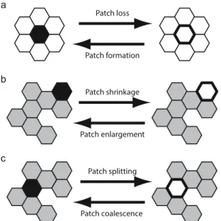
Accordingly, we systematically distinguish and analyse six elementary local events that can affect a patch (Fig. 2):
Patch formation is the appearance of a habitat site within a non-habitat area,
Patch loss is the event occurring when a habitat patch ceases to exist by the removal of its last site, Patch enlargement is the addition of a habitat site to an existing habitat patch,
Patch shrinkage is the removal of a habitat site from an existing habitat patch,
Patch coalescence is the joining of two habitat patches that were previously isolated, and Patch splitting is the division of a habitat patch into two or more isolated ones.
The event-based description of landscape dynamics enabled by the definition of these elementary events offers a general framework for studying patch dynamics in changing landscapes. Here, we apply this general framework to a simple DNLM, a random map with random local fluctuations. We also assume that the landscape-level hab- itat pattern is in a steady state when habitat loss occurs. We investigate the consequences of a single local habitat loss for the affected patch and analogously study the consequences of a single local habitat gain (see the corre- sponding loss/gain events in Fig. 2).
Our analysis underscores that landscape fragmentation is not only a problem resulting from the loss of con- nections between habitat patches, but also a problem related to a minimum feasible patch size. The habitat patches arising from dynamical habitat fragmentation may be smaller than the minimal area needed for sustaining a viable local population of the focal organism. Therefore, by removing a single unit of habitat, a potentially much larger area may be lost from the organism’s perspective. We estimate the magnitude of this kind of loss, and pre- dict the level q of habitat loss at which it is the most perilous.
Methods
The probabilities of the elementary events, as defined above, cannot be obtained analytically for a given landscape, as this would require the full enumeration of all patches together with their sizes and shapes. The number of possible patch shapes or configurations grows exponentially with patch size79–82. An enumeration of patch con- figurations has been achieved only up to a patch size of 45 sites83, later pushing this limit to 56 sites84. This poses
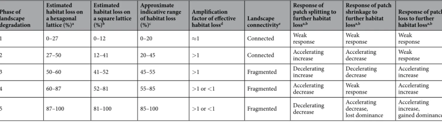
Phase of landscape degradation
Estimated habitat loss on a hexagonal lattice (%)a
Estimated habitat loss on a square lattice (%)b
Approximate indicative range of habitat loss (%)c
Amplification factor of effective
habitat lossd Landscape connectivitye
Response of patch splitting to further habitat lossa,b
Response of patch shrinkage to further habitat lossa,b
Response of patch loss to further habitat lossa,b
1 0–27 0–12 0–20 ≈1 Connected Weak
response Weak
response Weak
response
2 27–50 12–41 20–45 >1 Connected Accelerating
increase Accelerating
decrease Weak
response
3 50–60 41–52 45–55 >1 Fragmented Decelerating
increase Decelerating
decrease Accelerating increase
4 60–87 52–81 55–85 >1 or <1 Fragmented Accelerating
decrease Weak
response Accelerating increase
5 87–100 81–100 85–100 >1 or <1 Fragmented Decelerating
decrease
Accelerating decrease, lost dominance
Accelerating increase, gained dominance
Table 1. Five phases of habitat loss. aAccording to Fig. 3a. bAccording to Fig. 3b. cMean percentages from the preceding two columns rounded to the nearest 5%. dAccording to Fig. 3c,d. eAccording to percolation theory and as illustrated in Fig. 1.
a problem, since percolation maps without habitat patches larger than 56 sites are either very small or have very low values of p.
Therefore, we use Monte Carlo simulations to obtain the functions describing how the probabilities of the elementary events depend on the habitat cover p, by recording all events taking place on a percolation map with random fluctuations in site habitability. For this purpose, we use lattices consisting of N = 100 × 100 = 10,000 sites with periodic boundaries (i.e., the lattice is wrapped around a torus). Initially, pN randomly chosen sites are habitat sites and qN sites are non-habitat sites.
In our model, we assume a constant proportion q = 1 − p of non-habitat sites. Thus, when a randomly chosen habitat site is turned into a non-habitat site, at the same time a randomly chosen non-habitat site is turned into a habitat site. For each value of q, we record 6 · 106 elementary events. The record of an event consists of the type of the event and of the sizes of all the patches affected by the event. Since the total proportion of habitat sites does not change, the probabilities of patch loss and patch formation are equal, the probabilities of patch enlargement and patch shrinkage are equal, and the probabilities of patch splitting and patch coalescence are equal (see the pairs of opposing processes in Fig. 2). For this reason, it suffices to show results for the three elementary local events of patch loss, patch shrinkage, and patch splitting.
The probability of patch loss can be calculated analytically, assuming an infinite lattice. This enables us to compare our numerical results to an analytical baseline. Patch loss occurs when the local configuration matches the case shown in Fig. 2a. The probability of encountering such a local configuration at a random site of a hex- agonal lattice (also referred to as a honeycomb lattice or equilateral triangular lattice) is p(1 −p)6, whereas it is p(1 − p)4 on a square lattice (considering the von Neumann neighbourhood, i.e., the four nearest neighbours).
This example illustrates that the probabilities of elementary events are sensitive to the geometry of the considered lattice. Also the percolation threshold, which is analytically known for simple lattice geometries21, varies with the geometry of the considered lattice: pc= 0.5 (qc= 0.5) for the hexagonal lattice and pc= 0.592746 (qc= 0.407254) for the square lattice with a four-site neighbourhood. The threshold value is exact for the hexagonal lattice and is numerically estimated for the square lattice. In line with these differences, we must expect that the geometry of the lattice affects patch dynamics and the probabilities of the elementary events. For this reason, we include both the hexagonal lattice and the square lattice in our investigations.
For the hexagonal lattice, our numerical investigations are based on values of p ranging from 0.05 to 0.95 with 0.05 increments and from 0.45 to 0.55 with 0.01 increments; in addition, the values 0.57, 0.63, and 0.67 were also considered. For the square lattice, our numerical investigations are based on values of p ranging from 0.05 to 0.95 with 0.05 increments and from 0.45 to 0.80 with 0.01 increments.
Patch loss
Patch formation
Patch shrinkage
Patch enlargement
Patch splitting
Patch coalescence
a
b
c
Figure 2. Examples of elementary local events affecting habitat patches on a hexagonal lattice. Non-habitat sites are represented by white hexagons, while habitat sites are represented by grey hexagons. In each row, the hexagon with the thick black outline or black filling, respectively, is the focal one that changes from right to left or from left to right. The following descriptions refer to the elementary events occurring from left to right. (a) The loss of the focal habitat site causes the loss of the entire habitat patch, which consisted of a single site only.
(b) The loss of the focal habitat site from the perimeter of a habitat patch decreases the size of that patch. (c) The loss of the focal habitat site from a bottleneck of a habitat patch results in the splitting of that patch; in the shown example, the patch splits into two smaller patches (splitting into three smaller patches is possible for other patch configurations).
Results
In this section, we identify three kinds of landscape transitions that are important in addition to the traditionally recognized percolation transition. The resultant four transitions naturally subdivide the process of habitat loss into five phases. Finally, we show how the effective habitat loss experienced by organisms having different require- ments for minimal patch sizes increases with the actual habitat loss.
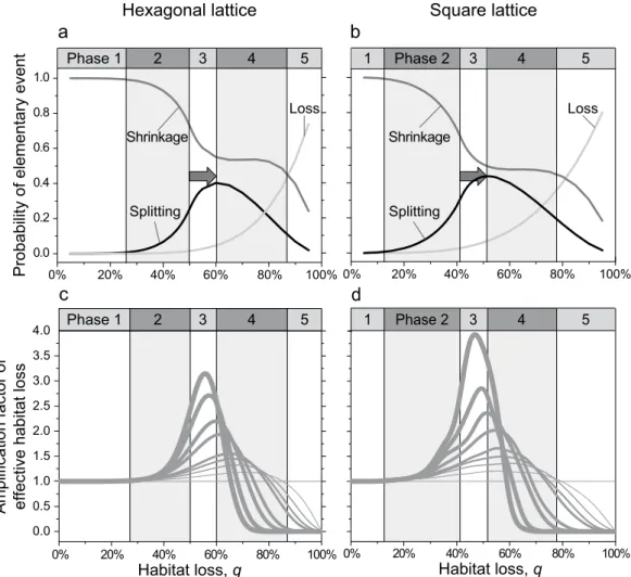
three impacts of habitat loss. The functions describing how the probabilities of patch loss, patch shrink- age, and patch splitting change with the level of habitat loss q turn out to have similar shapes for the hexagonal lattice and the square lattice (Fig. 3a,b). The numerically obtained probabilities of patch loss perfectly match the aforementioned analytical predictions, increasing monotonically as the level of habitat loss q is raised. The prob- ability of patch splitting reaches its maximum at a value of q that is higher than the percolation threshold (q > qc).
b a
0% 20% 40% 60% 80% 100%
0% 20% 40% 60% 80% 100%
0.0 0.2 0.4 0.6 0.8 1.0
Probability of elementary event
Loss Shrinkage
Splitting
Loss Shrinkage
Splitting
Square lattice Hexagonal lattice
Phase 1 2 3 4 5 1 Phase 2 3 4 5
20% 40% 60% 80% 100%
0% 20% 40% 60% 80% 100%
Amplification factor of effective habitat loss
Habitat loss, q Habitat loss,q
c d
Phase 1 2 3 4 5 1 Phase 2 3 4 5
0%
0.0 0.5 1.0 1.5 2.0 2.5 3.0 3.5 4.0
Figure 3. Probabilities of elementary local events affecting habitat patches on a (a) hexagonal lattice and (b) square lattice, together with the corresponding amplification factors of effective habitat loss on a
(c) hexagonal lattice and (d) square lattice. The curves in panels a and b show how the probabilities of patch loss (light-grey curves), patch shrinkage (dark-grey curves), and patch splitting (black curves) vary with the level of habitat loss q. The vertical lines indicate the thresholds separating the five phases of habitat loss identified in this study, which are indicated by alternating white and light-grey backgrounds. Note that for both lattice geometries, the probability of patch splitting peaks at levels of habitat loss that are larger than the percolation threshold; the differences are highlighted by the grey arrows. In panels c and d, the vertical axis shows the amplification factor of effective habitat loss, i.e., the average number of habitat sites lost from a population’s living area caused by the loss of one habitat site, when habitat patches of at least m habitat sites are required to sustain a viable local population. The horizontal line shows the amplification factor of effective habitat loss for m = 1, in which case the removal of a single habitat site always causes the loss of no more and no less than one habitat site from the population’s living area. The thickness of the curves increases with increasing m from 1 up to 9 sites. Notice that the maximum amplification factors of effective habitat loss are observed for levels of habitat loss q in excess of the percolation threshold situated at the transition between Phases 2 and 3. Also note that for high levels of habitat loss, very few habitat patches remain viable, which means that most removals of habitat sites affect habitat patches in which the population is not viable, resulting in the amplification factor of effective habitat loss converging to zero.
For the hexagonal lattice, patch splitting is most probable when ca. 60% of the habitat is lost (Fig. 3a), while for the square lattice this peak occurs at ca. 50% of habitat loss (Fig. 3b). From there up to ca. 80% of habitat loss, the probability of patch shrinkage remains relatively constant, independent of the two considered lattice geometries (Fig. 3a,b).
four transitions caused by habitat loss. We observe the probabilities of the elementary events during the degradation from a pristine landscape (q = 0) to the disappearance of all habitat (q = 1). Based on the results shown in Fig. 3, we propose to divide the process of habitat loss into five phases, each corresponding to a certain interval of habitat loss. The boundaries between adjacent phases are determined by four major transitions in landscape structure and dynamics occurring during the course of landscape degradation:
Transition 1 (occurring at a level of habitat loss of ca. 20%). Appearance of isolated patches and a very slowly increasing incidence of patch splitting. This transition can be defined to occur at the level of habitat loss q at which the probability of patch shrinkage falls below 99%.
Transition 2 (occurring at a level of habitat loss of ca. 45%). Transition from a fully connected to a fragmented landscape. This transition happens at the percolation threshold, which is defined in, and well known from, the literature on percolation processes21.
Transition 3 (occurring at a level of habitat loss of ca. 55%). Switch from an increasing to a decreasing probability of patch splitting. This transition is thus defined to occur at the level of habitat loss q at which the patch-splitting probability peaks.
Transition 4 (occurring at a level of habitat loss of ca. 85%). Sudden decline in the probability of patch shrink- age. This transition happens when the probability of patch loss starts to dominate, and we can define it to occur at the habitat loss q at which the probability of patch loss surpasses the probabilities of patch shrinkage and patch splitting.
The four values of habitat loss q listed above are just rough indications, mentioned here only for the sake of approximate orientation. Naturally, the exact values depend on the details of the model, and in particular on the considered lattice geometry (Table 1).
five phases of habitat loss. The aforementioned four transitions naturally divide a landscape’s degradation process into five phases (Table 1; see Fig. 1 for illustration):
Phase 1 (occurring at levels of habitat loss from 0% to ca. 20%; Fig. 1a). The landscape is dominated by a single large habitat patch, known from percolation theory as a spanning cluster, which spans across the entire landscape.
By far, the most frequent event during this phase is the shrinkage of the spanning patch (Fig. 3a,b). In contrast, patch splitting and patch loss are rare events, as they happen only to the non-spanning smaller patches (Fig. 3a,b).
Throughout this phase, all three event probabilities remain almost constant (Fig. 3a,b).
Phase 2 (occurring at levels of habitat loss from ca. 20% to ca. 45%; Fig. 1b). The spanning patch still exists, but the number and size of the non-spanning smaller patches become significant. Close to the percolation threshold at this phase’s upper boundary, the spanning patch is filamental, which means that the random removal of a single habitat site in the considered lattices of 100 × 100 sites results in its splitting into two habitat patches in about 1/4 of the cases (Fig. 3a,b). In this phase, patch shrinkage and patch splitting co-occur at appreciable frequencies, while patch loss remains rare (Fig. 3a,b). The sensitivities of the frequencies of patch shrinkage and patch splitting to habitat loss (slopes in Fig. 3a,b) both increase toward the percolation threshold, where they reach their peaks.
Phase 3 (occurring at levels of habitat loss from ca. 45% to ca. 55%; Fig. 1c). This phase is similar to the pre- vious one in terms of the occurrence of the elementary events, while being characterized by a key difference in landscape structure: as habitat loss q exceeds the percolation threshold qc, the landscape is fragmented. In the theoretical limit of infinite landscape size, no spanning patch would exist anymore; however, for finite land- scapes, we may still find a spanning patch when q − qc is small, but the probability of such configurations rapidly declines with an increase of q − qc and/or of landscape size21. This fragmentation implies that it is not possible for a population to spread across the landscape without being obstructed by non-habitat sites, which poses a serious burden on its persistence (see23 for a review). In this phase, the frequencies of patch shrinkage and patch splitting continue to decrease and increase, respectively, while the frequency of patch loss also increases, but still remains at low levels (Fig. 3a,b). The sensitivities of the frequencies of patch shrinkage and patch splitting to habitat loss (slopes in Fig. 3a,b) both decrease above the percolation threshold, where they had reached their peaks (Fig. 3a,b).
Phase 4 (occurring at levels of habitat loss from ca. 55% to ca. 85%; Fig. 1d). In this phase, the frequency of patch shrinkage is surprisingly unresponsive to the further increase of habitat loss, exhibiting a broad plateau (Fig. 3a,b). After having reached its peak at the transition between Phases 3 and 4, the frequency of patch splitting declines with the further increase of habitat loss, and patch loss is gaining importance, gradually becoming as frequent as patch shrinkage (Fig. 3a,b). These effects are caused by decreasing patch sizes.
Phase 5 (occurring at levels of habitat loss from ca. 85% to 100%; Fig. 1e). In this final phase of landscape deg- radation, the frequency of patch loss continues to increase super-linearly with further habitat loss, exceeding the frequencies of patch shrinkage and patch splitting, with the latter both continuing to decline with further habitat loss (Fig. 3a,b). Populations inhabiting these kinds of landscapes are confined to live primarily in small habitat patches, which are frequently lost. Therefore, sufficient dispersal between waxing and waning habitat patches is crucial for a population’s persistence.
The aforementioned phases can be observed on a hexagonal lattice (Fig. 3a) and on a square lattice with von Neumann neighbourhood (Fig. 3b). In the hexagonal lattice, each phase starts later, i.e., at a higher level of habitat
loss (Table 1). The reason for this is the higher number of connections per site (degree): each site is connected to six others, as opposed to four others in the square lattice with von Neumann neighbourhood. Therefore, more sites need to be removed from a hexagonal lattice for causing a habitat patch to split, or for isolating a habitat site completely, making it less vulnerable to patch loss.
Effective habitat loss. To assess the severity of impact of landscape degradation on a population, we assume that sustaining a viable local population requires a habitat patch with a minimum of m habitat sites. When a single isolated habitat site is sufficient for sustaining a local population (m = 1), then every site removal decreases the population’s living area by exactly one site. In contrast, when m = 2, then fragmentation of a habitat patch of size 3 creates two fragments, each of size 1, which effectively removes three habitat sites from the population’s living area. In this manner, every elementary local event is evaluated according to the effective habitat loss it causes.
Some site removals cause no loss of habitat, as they affect patches that are already too small to sustain a local population. These habitat patches are part of the landscape; they are just lost from the population’s living area.
For any given total level of habitat loss q, we determine the amplification factor of effective habitat loss by averaging the effective habitat loss (i.e., the loss of a population’s living area) over a large number of elementary events (6 · 106), each involving an actual habitat loss of one habitat site. This factor starts to exceed 1 appreciably when the level of habitat loss q exceeds roughly 30% (Fig. 3c,d), which is well below the percolation threshold and roughly coincides with the transition from Phase 1 to Phase 2. The amplification factor of effective habitat loss peaks at levels of habitat loss well above the percolation threshold, close to the level of habitat loss at which the probability of patch splitting is maximal (compare Fig. 3a–d). This peak shifts toward lower levels of habitat loss q as the minimal patch area needed for a viable local population increases (Fig. 3c,d). After reaching its peak, the amplification factor of effective habitat loss strongly declines and typically drops below 1 in Phase 4 (Fig. 3c,d), which means that by removing a single habitat site on average less than one habitat site is lost from the popula- tion’s living area. This is because in this phase most habitat patches are already too small for sustaining a local population, so that the further removal of a habitat site often causes no further loss from a population’s living area.
Naturally, this effect is stronger and starts earlier, i.e., at lower levels of habitat loss q, for populations requiring habitat patches of larger minimal size m.
Discussion
Here we have presented a dynamical view of habitat loss by observing the probabilities of elementary local events on the spatial mesoscale of individual habitat patches. Our framework for studying changing landscapes allows us to identify three additional landscape transitions beside the one associated with the well-known percolation threshold. The four corresponding thresholds demarcate five distinct phases of habitat loss. Phase 1 begins from a pristine habitat and is characterized by the shrinkage of contiguous habitat area. In Phase 2, detached habitat patches begin to appear, even though a spanning patch still exists. The percolation threshold marks the transi- tion to Phase 3, in which the effective habitat loss peaks, and at the end of which the frequency of patch splitting reaches its peak. It is important to emphasize that – although the connectivity of habitat sites plummets at the percolation threshold – our results demonstrate that the severity and frequency of patch splitting peaks at higher levels of habitat loss. It is in Phase 3 that organisms requiring a larger number of habitat sites for sustaining a viable local population experience a peak in effective habitat loss. Phase 4 commences with the peak in the probability of patch splitting and is characterized by a nearly constant probability of patch shrinkage. Finally, in Phase 5, habitat loss is so severe that the landscape mainly consists of isolated habitat sites, which then disappear one-by-one as habitat cover decreases.
The same process can alternatively be described from the opposite direction, which is a trend toward habitat gain. For example, when sites with arable land are created, the corresponding habitat patches may become suitable for weeds or other agricultural pests, increasing their population sizes, as well as their probabilities of spreading across the landscape.
Dynamical Neutral Landscape Models (DNLMs) serve as natural benchmarks and references to which data observed on real landscapes can be compared. High correlations between a landscape index and a response var- iable measured on artificial landscapes have often been confirmed by measurements on real landscapes16. Real landscapes differ from percolation maps in at least two important characteristics. (1) Non-habitat patches can be traversed up to some distance85–87, and thus, habitat patches can still be functionally connected14 in spite of their physical fragmentation. (2) Real landscapes are, in general, not as randomly structured as percolation maps, but instead exhibit some degree of aggregation34,88–90. When habitat sites are aggregated, patch splitting is less likely, and thus occurs at higher levels of habitat loss. This is corroborated, for example, by observations on birds and mammals85, which have led to the conclusion that a landscape becomes significantly fragmented for these species only when 60–70% of the habitat is destroyed. Habitat fragmentation on a percolation map can thus be considered as a worst-case scenario.
Our numerical investigations in the present study have been carried out on a percolation map, since this is the first20 and best-studied NLM, and also the most widely used in spatially explicit models13,15,30,67,68,91–94. Percolation maps are often applied to study habitat fragmentation because of the critical behaviour they exhibit13,20–22. In contrast, habitat change in other models of spatial ecology has mostly been defined in terms of disturbance regimes13,15,91,95–100. Up to now, NLMs with temporal changes have scarcely been considered (for exceptions, see23,24,48,56,69,73). The DNLM framework could be extended in a variety of ways. First, the dynamical properties of NLMs other than percolation maps could be similarly investigated. This perspective could also be applied to landscape models defined in continuous space (rather than on a lattice, as in our present study): In those contexts, it would then be interesting to examine how the dynamical landscape properties are changing when scanning through ranges of distances for defining whether nearby locations are regarded as being connected or not. The frequency distribution of events on other landscapes is expected to be different. In particular, on landscapes with
spatially aggregated patterns of habitat sites, we expect patch splitting to dominate at higher levels of habitat loss.
Second, the dynamics of populations can be described in greater mechanistic detail. For example, the costly – but in general not impossible – movement of individuals through non-habitat sites could be included (for an exam- ple of such a model, see57). The explicit study of population dynamics within the patches, including the study of extinction times, is also a promising direction for future research (see23 about connecting habitat dynamics and population dynamics in a percolation-theoretical framework). Third, in our present study, we have removed habitat sites randomly, according to a spatially uniform probability distribution. Future research could consider more elaborate models of habitat loss, reflecting real-word processes such as agricultural land-use expansion or other anthropogenic environmental changes. In this context, an examination of contagious habitat loss101 would be of particular interest.
The importance of the percolation threshold for understanding landscape dynamics and habitat fragmen- tation has been recognized in the literature from the early days of landscape ecology20 (see reviews of relevant studies in58,102). Here we have suggested considering three additional thresholds that are fundamentally related to understanding the dynamics of habitat patches and the impacts of habitat loss on different organisms that require habitat patches of a certain minimal size for their local survival. Altogether, the four thresholds we have defined, examined, and discussed here distinguish five characteristic phases of habitat loss. We believe that the distinction between these phases according to a landscape’s dynamical properties, focussing on the patch-scale events, is crucial for the protection of species subject to habitat loss and fragmentation. In particular, important qualitative changes in the dynamics of habitat patches can be revealed by studying the frequencies of the elementary local events we have investigated here. Habitat changes thus becoming detectable will often foreshadow critical land- scape transitions to occur, which allows scientists and managers to take action before disastrous and irreversible damage is done.
Data Availability
The datasets generated and analysed for the current study are available from the corresponding author on rea- sonable request.
References
1. Foley, J. A. et al. Global consequences of land use. Science 309, 570–574, https://doi.org/10.1126/science.1111772 (2005).
2. Fahrig, L. Effects of habitat fragmentation on biodiversity. Annu. Rev. Ecol. Evol. Syst. 34, 487–515, https://doi.org/10.1146/annurev.
ecolsys.34.011802.132419 (2003).
3. Fischer, J. & Lindenmayer, D. B. Landscape modification and habitat fragmentation: a synthesis. Global Ecol. Biogeogr. 16, 265–280, https://doi.org/10.1111/j.1466-8238.2007.00287 (2007).
4. Haddad, N. M. et al. Habitat fragmentation and its lasting impact on Earth’s ecosystems. Science Advances 1, e1500052, https://doi.
org/10.1126/sciadv.1500052 (2015).
5. Pfeifer, M. et al. Creation of forest edges has a global impact on forest vertebrates. Nature 551, 187, https://doi.org/10.1038/
nature24457 (2017).
6. Primack, R. B. Essentials of Conservation Biology (Sinauer Associates, 1998).
7. Lindenmayer, D. B. & Fischer, J. Tackling the habitat fragmentation panchreston. Trends Ecol. Evol. 22, 127–132, https://doi.
org/10.1016/j.tree.2006.11.006 (2007).
8. Fazey, I., Fischer, J. & Lindenmayer, D. B. What do conservation biologists publish? Biol. Conserv. 124, 63–73, https://doi.
org/10.1016/j.biocon.2005.01.013 (2005).
9. Fardila, D., Kelly, L. T., Moore, J. L. & McCarthy, M. A. A systematic review reveals changes in where and how we have studied habitat loss and fragmentation over 20 years. Biol. Conserv. 212, 130–138, https://doi.org/10.1016/j.biocon.2017.04.031 (2017).
10. Hansson, L. & Angelstam, P. Landscape ecology as a theoretical basis for nature conservation. Landscape Ecol. 5, 191–201 (1991).
11. Hargis, C. D., Bissonette, J. A. & David, J. L. The behaviour of landscape metrics commonly used in the study of habitat fragmentation. Landscape Ecol. 13, 167–186 (1998).
12. Tischendorf, L. & Fahrig, L. How should we measure landscape connectivity? Landscape Ecol. 15, 633–641 (2000).
13. With, K. A. & Crist, T. O. Critical threshold in species responses to landscape structure. Ecology 76, 2446–2459 (1995).
14. Andrén, H. Population responses to habitat fragmentation: statistical power and the random sample hypothesis. Oikos 235–242 (1996).
15. Neuhauser, C. Habitat destruction and competitive coexistence in spatially explicit models with local interaction. J. Theor. Biol. 193, 445–463 (1998).
16. Tischendorf, L. Can landscape indices predict ecological processes consistently? Landscape Ecol. 16, 235–254 (2001).
17. Söngerath, D. & Schröder, B. Population dynamics and habitat connectivity affecting the spatial spread of populations – a simulation study. Landscape Ecol 17, 57–70 (2002).
18. Solé, R. V. & Bascompte, J. Habitat loss and extinction thresholds. In Self-Organization in Complex Ecosystems (eds Solé, R. V. &
Bascompte, J.) 171–214 (Princeton University Press, 2006).
19. With, K. A. & King, A. W. The use and misuse of neutral landscape models in ecology. Oikos 79, 219–229 (1997).
20. Gardner, R. H., Milne, B. T., Turner, M. G. & O’Neill, R. V. Neutral models for the analysis of broad-scale landscape pattern.
Landscape Ecol. 1, 19–28 (1987).
21. Stauffer, D. & Aharony, A. Introduction to Percolation Theory. Revised Second Edn (Taylor and Francis, 1994).
22. Boswell, G. P., Britton, N. F. & Franks, N. R. Habitat fragmentation, percolation theory and the conservation of a keystone species.
Proc. R. Soc. London, Ser. B 265, 1921–1925 (1998).
23. Oborny, B., Szabó, G. & Meszéna, G. In Scaling Biodiversity (eds Storch, D., Marquet, P. A. & Brown, J. H.) 409–440 (Cambridge University Press, 2007).
24. Kun, Á. Generation of temporally and spatially heterogeneous landscapes for models of population dynamics. Appl. Ecol. Environ.
Res. 4, 73–84 (2007).
25. Stoddard, S. T. Continuous versus binary representations of landscape heterogeneity in spatially-explicit models of mobile populations. Ecol. Model. 221, 2409–2414, https://doi.org/10.1016/j.ecolmodel.2010.06.024 (2010).
26. Keitt, T. H. & Johnson, A. R. Spatial heterogeneity and anomalous kinetics: emergent patterns in diffusion-limited predator-prey interaction. J. Theor. Biol. 171, 127–139 (1995).
27. Milne, B. T., Keitt, T. H., Hatfield, C. A., David, J. & Hraber, P. T. Detection of critical densities associated with pinion-juniper woodland ecotones. Ecology 77, 805–821 (1996).
28. Gastner, M., Oborny, B., Pruessner, G. & Zimmermann, D. Transition from connected to fragmented vegetation across an environmental gradient: scaling laws in ecotone geometry. Am. Nat. 174, 23–39 (2009).
29. Gustafson, E. J. & Parker, G. R. Relationships between landcover proportions and indices of landscape spatial pattern. Landscape Ecol. 7, 101–110 (1992).
30. Hiebeler, D. Populations on fragmented landscapes with spatially structured heterogeneities: landscape generation and local dispersal. Ecology 81, 1629–1641 (2000).
31. Huth, G., Lesne, A., Munoz, F. & Pitard, E. Correlated percolation models of structured habitat in ecology. Physica A: Statistical Mechanics and its Applications 416, 290–308, https://doi.org/10.1016/j.physa.2014.08.006 (2014).
32. O’Neill, R. V., Gardner, R. H. & Turner, M. G. A hierarchical neutral model for landscape analysis. Landscape Ecol. 7, 55–61 (1992).
33. Johnson, G. D., Myers, W. L. & Patil, G. P. Stochastic generating models for simulating hierarchically structured multi-cover landscapes. Landscape Ecol. 14, 413–421 (1999).
34. Turner, M. G. Spatial simulation of landscape changes in Georgia: A comparison of 3 transition models. Landscape Ecol. 1, 29–36 (1987).
35. Gaucherel, C. Neutral models for polygonal landscapes with linear networks. Ecol. Model. 219, 39–48, https://doi.org/10.1016/j.
ecolmodel.2008.07.028 (2008).
36. Gaucherel, C., Fleury, D., Auclair, D. & Dreyfus, P. Neutral models for patchy landscapes. Ecol. Model. 197, 159–170, https://doi.
org/10.1016/j.ecolmodel.2006.02.044 (2006).
37. With, K. A., Gardner, R. H. & Turner, M. G. Landscape connectivity and population distribution in heterogeneous environments.
Oikos 78, 151–169 (1997).
38. Palmer, M. W. The coexistence of species in fractal landscapes. Am. Nat. 139, 375–397 (1992).
39. Hovestadt, T., Messer, S. & Poethke, H. J. Evolution of reduced dispersal mortality and “fat-tailed” dispersal kernels in autocorrelated landscapes. Proc. R. Soc. London, Ser. B 268, 385–391 (2001).
40. Kashian, D. M., Sosin, J. R., Huber, P. W., Tucker, M. M. & Dombrowski, J. A neutral modeling approach for designing spatially heterogeneous jack pine plantations in northern Lower Michigan, USA. Landscape Ecol. 32, 1117–1131, https://doi.org/10.1007/
s10980-017-0514-y (2017).
41. van Strien, M. J., Slager, C. T. J., de Vries, B. & Grêt-Regamey, A. An improved neutral landscape model for recreating real landscapes and generating landscape series for spatial ecological simulations. Ecology and Evolution 6, 3808–3821, https://doi.
org/10.1002/ece3.2145 (2016).
42. Etherington, T. R., Holland, E. P. & O’Sullivan, D. NLMpy: a python software package for the creation of neutral landscape models within a general numerical framework. Methods in Ecology and Evolution 6, 164–168, https://doi.org/10.1111/2041-210X.12308 (2015).
43. Kirkpatrick, L. A. & Weishampel, J. F. Quantifying spatial structure of volumetric neutral models. Ecol. Model. 186, 312–325, https://doi.org/10.1016/j.ecolmodel.2005.01.056 (2005).
44. Czárán, T. Spatiotemporal Models of Population and Community Dynamics (Chapman and Hall, 1998).
45. Tilman, D. & Kareiva, P. Spatial Ecology: The Role of Space in Population Dynamics and Interspecific Interactions (Princeton University Press, 1997).
46. Dieckmann, U., Law, R. & Metz, J. A. J. The Geometry of Ecological Interactions: Simplifying Spatial Complexity (Cambridge University Press, 2000).
47. Bascompte, J. & Solé, R. V. Habitat fragmentation and extinction threshold in spatially explicit models. J. Anim. Ecol. 65, 465–473 (1996).
48. Szabó, G., Gergely, H. & Oborny, B. Generalized contact process on random environments. Phys. Rev. E: Stat. Phys. Plasmas, Fluids 65, 066111 (2002).
49. Kun, Á. & Oborny, B. Survival and competition of clonal plant populations in spatially and temporally heterogeneous habitats.
Community Ecology 4, 1–20 (2003).
50. Ezard, T. H. G. & Travis, J. M. J. The impact of habitat loss and fragmentation on genetic drift and fixation time. Oikos 114, 367–375, https://doi.org/10.1111/j.2006.0030-1299.14778.x (2006).
51. Le Ber, F. et al. Neutral modelling of agricultural landscapes by tessellation methods – Application for gene flow simulation. Ecol.
Model. 220, 3536–3545, https://doi.org/10.1016/j.ecolmodel.2009.06.019 (2009).
52. Wimberly, M. C. Species dynamics in disturbed landscapes: when does a shifting habitat mosaic enhance connectivity? Landscape Ecol. 21, 35–46, https://doi.org/10.1007/s10980-005-7757-8 (2006).
53. Schrott, G. R., With, K. A. & King, A. W. On the importance of landscape history for assessing extinction risk. Ecol. Appl. 15, 493–506 (2005).
54. Graves, T. A. et al. The influence of landscape characteristics and home-range size on the quantification of landscape-genetics relationships. Landscape Ecol. 27, 253–266, https://doi.org/10.1007/s10980-011-9701-4 (2012).
55. Dytham, C. The effect of habitat destruction pattern on species persistence: a cellular model. Oikos 74, 340–344 (1995).
56. Gaucherel, C. Self-organization of patchy landscapes: hidden optimization of ecological processes. Journal of Ecosystem &
Ecography 1, 105, https://doi.org/10.4172/2157-7625.1000105 (2011).
57. Oborny, B. & Hubai, A. G. Patch size and distance: modelling habitat structure from the perspective of clonal growth. Ann. Bot.
114, 389–398, https://doi.org/10.1093/aob/mcu110 (2014).
58. Oborny, B., Benedek, V., Englert, P., Gulyás, M. & Hubai, A. G. The plant in the labyrinth: Adaptive growth and branching in heterogeneous environments. J. Theor. Biol. 412, 146–153, https://doi.org/10.1016/j.jtbi.2016.10.015 (2017).
59. Fransen, B., de Kroon, H. & Berendse, F. Soil nutrient heterogeneity alters competition between perennial grass species. Ecology 82, 2534–2546 (2001).
60. Wijesinghe, D. K. & Hutchings, M. J. The effects of spatial scale of environmental heterogeneity on the growth of a clonal plant: an experimental study with Glechoma hederacea. J. Ecol. 85, 17–28 (1997).
61. Wijesinghe, D. K. & Hutchings, M. J. The effect of environmental heterogeneity on the performance of Glechoma hederacea: the interactions between patch contrast and patch scale. J. Ecol. 87, 860–872 (1999).
62. Wijesinghe, D. K. & Handel, S. N. Advantages of clonal growth in heterogeneous habitats: an experiment with Potentilla simplex. J.
Ecol. 82, 495–502 (1994).
63. Wiens, J. A., Schooley, R. L. & Weeks, D. Jr. Patchy landscapes and animal movements: do beetles percolate? Oikos 78, 257–264 (1997).
64. McIntyre, N. E. & Wiens, J. A. Interaction between habitat abundance and configuration: experimental validation of some predictions from percolation theory. Oikos 88, 129–137 (1999).
65. With, K. A., Pavuk, D. M., Worchuck, J. L., Oates, R. K. & Fisher, J. L. Threshold effects of landscape structure on biological control in agroecosystems. Ecol. Appl. 12, 52–65, https://doi.org/10.1890/1051-0761(2002)012[0052:teolso]2.0.co;2 (2002).
66. With, K. & Pavuk, D. Habitat area trumps fragmentation effects on arthropods in an experimental landscape system. Landscape Ecol. 26, 1035–1048, https://doi.org/10.1007/s10980-011-9627-x (2011).
67. Magyar, G., Kun, A., Oborny, B. & Stuefer, J. F. Importance of plasticity and decision-making strategies for plant resource acquisition in spatio-temporally variable environments. New Phytol. 174, 182–193, https://doi.org/10.1111/j.1469-8137.2007.01969.x (2007).
68. Kun, Á., Oborny, B. & Dieckmann, U. Intermediate landscape disturbance maximizes metapopulation density. Landscape Ecol. 24, 1341–1350, https://doi.org/10.1007/s10980-009-9386-0 (2009).
69. Hagen-Zanker, A. & Lajoie, G. Neutral models of landscape change as benchmarks in the assessment of model performance.
Landscape Urban Plann. 86, 284–296 (2008).
70. Hiebeler, D. E., Houle, J., Drummond, F., Bilodeau, P. & Merckens, J. Locally dispersing populations in heterogeneous dynamic landscapes with spatiotemporal correlations. I. Block disturbance. J. Theor. Biol. 407, 212–224, https://doi.org/10.1016/j.
jtbi.2016.07.031 (2016).
71. Hiebeler, D. E. & Hill, J. L. Locally dispersing populations in heterogeneous dynamic landscapes with spatiotemporal correlations.
II. Habitat driven by voter dynamics. J. Theor. Biol. 407, 81–89, https://doi.org/10.1016/j.jtbi.2016.07.033 (2016).
72. Hiebeler, D. E. & Morin, B. R. The effect of static and dynamic spatially structured disturbances on a locally dispersing population.
J. Theor. Biol. 246, 136–144, https://doi.org/10.1016/j.jtbi.2006.12.024 (2007).
73. Keymer, J. E., Marquet, P. A., Velasco-Hernández, J. X. & Levin, S. A. Extinction threshold and metapopulation persistence in dynamic landscapes. Am. Nat. 156, 478–494 (2000).
74. Fransen, B., Blijjenberg, J. & De Kroon, H. Root morphological and physiological plasticity of perennial grass species and the exploitation of spatial and temporal heterogeneous nutrient patches. Plant Soil 211, 179–189 (1999).
75. Forman, R. T. T. Land Mosaics: The Ecology of Landscapes and Regions (Cambridge University Press, 1995).
76. Jaeger, J. A. G. Landscape division, splitting index, and effective mesh size: new measures of landscape fragmentation. Landscape Ecol. 15, 115–130 (2000).
77. Akçakaya, H. R. E. Linking population-level risk assessment with landscape and habitat models. Sci. Total Environ. 274, 283–291, https://doi.org/10.1016/S0048-9697(01)00750-1 (2001).
78. Didham, R. K., Kapos, V. & Ewers, R. M. Rethinking the conceptual foundations of habitat fragmentation research. Oikos 121, 161–170, https://doi.org/10.1111/j.1600-0706.2011.20273.x (2012).
79. Sykes, M. F. & Glen, M. Percolation processes in two dimensions. I. Low-density series expansion. J. Phys. A: Math. Gen 9, 87–95 (1976).
80. Margolina, A., Djordjevic, Z. V., Stauffer, D. & Stanley, H. E. Corrections to scaling for branched polymers and gels. Phys. Rev. B 28, 1652–1654 (1983).
81. Mertens, S. Lattice animals: A fast enumeration algorithm and new perimeter polynomials. J. Stat. Phys. 58, 1095–1108 (1990).
82. Mertens, S. & Lautenbacher, M. E. Counting lattice animals: A parallel attack. J. Stat. Phys. 66, 669–678 (1992).
83. Jensen, I. Enumeration of lattice animals and trees. J. Stat. Phys 102, 865–881 (2001).
84. Jensen, I. Series for lattice animals or polyominoes, http://www.ms.unimelb.edu.au/~iwan/animals/series/square.site.ser (2004).
85. Andrén, H. Effect of habitat fragmentation on birds and mammals in landscapes with different proportion of suitable habitat: a review. Oikos 71, 355–366 (1994).
86. Wiens, J. A. In Dispersal (eds Clobert, J., Danchin, E., Dhondt, A. A. & Nichols, J. D.) 96–109 (Oxford University Press, 2001).
87. Bowne, D. R. & Bowers, M. A. Interpatch movements in spatially structured populations: a literature review. Landscape Ecol. 19, 1–20 (2004).
88. Matlack, G. R. & Leu, N. A. Persistence of dispersal-limited species in structured dynamic landscapes. Ecosystems 10, 1287–1298 (2007).
89. Neel, M. C., McGarigal, K. & Cushman, S. A. Behavior of class-level landscape metrics across gradients of class aggregation and area. Landscape Ecol. 19, 435–455, https://doi.org/10.1023/B:LAND.0000030521.19856.cb (2004).
90. Ovaskainen, O., Sato, K., Bascompte, J. & Hanski, I. Metapopulation models for extinction threshold in spatially correlated landscapes. J. Theor. Biol. 215, 95–108, https://doi.org/10.1006/jtbi.2001.2502 (2002).
91. Turner, M. G., Gardner, R. H., Dale, V. H. & O’Neill, R. V. Predicting the spread of disturbance across heterogeneous landscapes.
Oikos 55, 121–129 (1989).
92. Oborny, B. & Kun, Á. Fragmentation of clones: how does it influence dispersal and competitive ability? Evol. Ecol. 15, 319–346 (2002).
93. Oborny, B., Czárán, T. & Kun, Á. Exploration of resource patches by clonal growth: a spatial model on the effect of transport between modules. Ecol. Model. 141, 151–169 (2001).
94. Oborny, B., Kun, Á., Czárán, T. & Bokros, S. The effect of clonal integration on plant competition for mosaic habitat space. Ecology 81, 3291–3304 (2000).
95. Inghe, O. Genet and ramet survivorship under different mortality regimes – A cellular automata model. J. Theor. Biol. 138, 257–270 (1989).
96. Franklin, J. F. & Forman, R. T. T. Creating landscape pattern by forest cutting: Ecological consequences and principles. Landscape Ecol. 1, 5–18 (1987).
97. Savage, M., Sawhill, B. & Askenazi, M. Community dynamics: what happens when we rerun the tape. J. Theor. Biol. 205, 515–526 (2000).
98. Lavorel, S., O’Neill, R. V. & Gardner, R. H. Spatio-temporal dispersal strategies and annual plant species coexistence in a structured landscape. Oikos 71, 75–88 (1994).
99. Winkler, E. & Fischer, M. The role of vegetative spread and seed dispersal for optimal life histories of clonal plants: a simulation study. Evol. Ecol. 15, 281–301 (2002).
100. Campos, P. R. A., Neto, E. D. C., Oliveira, V. M. D. & Gomes, M. A. F. Neutral communities in fragmented landscapes. Oikos 121, 1737–1748 (2012).
101. Boakes, E. H., Mace, G. M., McGowan, P. J. K. & Fuller, R. A. Extreme contagion in global habitat clearance. Proc. R. Soc. London, Ser. B 277, 1081–1085, https://doi.org/10.1098/rspb.2009.1771 (2010).
102. Solé, R. V., Bartumeus, F. & Gamarra, J. P. G. Gap percolation in rainforests. Oikos 110, 177–185 (2005).
Acknowledgements
We thank Ferenc Jordán, Gabriella Magyar, and Péter Mandl for their helpful comments on earlier versions of this manuscript. Péter Englert kindly allowed us to use his graphical modelling tool PLA-MAZE for producing the pictures in Fig. 1. We are also very grateful to Géza Meszéna and György Szabó for enjoyable discussions about our project. This work was supported by the Hungarian National Research Fund and the National Research, Development and Innovation Office (NKFIH) under the grant numbers T29789, T35009, K109215, K124438, K100299, K119347, GINOP-2.3.2-15-2016-00057, GINOP-2.3.2-15-2016-00019, and NWO-OTKA N34028.
Á.K. is grateful for support from the European Science Foundation (TBA/01) for his participation in the Young Scientists Summer Program of the International Institute for Applied Systems Analysis in Laxenburg, Austria, and for support for a János Bolyai Research Fellowship from the Hungarian Academy of Sciences. B.O. acknowledges support by the International Program of the Santa Fe Institute, USA. U.D. gratefully acknowledges support by the Sixth Framework Program of the European Commission, the European Science Foundation, the Austrian Science Fund, the Austrian Ministry of Science and Research, and the Vienna Science and Technology Fund.
Author contributions
Á.K., B.O. and U.D. jointly devised the study and wrote the manuscript. Á.K. implemented the numerical investigations and analysed the data. All authors reviewed and approved the manuscript.
Additional information
Competing Interests: The authors declare no competing interests.
Publisher’s note: Springer Nature remains neutral with regard to jurisdictional claims in published maps and institutional affiliations.
Open Access This article is licensed under a Creative Commons Attribution 4.0 International License, which permits use, sharing, adaptation, distribution and reproduction in any medium or format, as long as you give appropriate credit to the original author(s) and the source, provide a link to the Cre- ative Commons license, and indicate if changes were made. The images or other third party material in this article are included in the article’s Creative Commons license, unless indicated otherwise in a credit line to the material. If material is not included in the article’s Creative Commons license and your intended use is not per- mitted by statutory regulation or exceeds the permitted use, you will need to obtain permission directly from the copyright holder. To view a copy of this license, visit http://creativecommons.org/licenses/by/4.0/.
© The Author(s) 2019