Kétdimenziós mesterséges festési eljárások. Hatások és alkalmazások

(1)

University of Pannonia Veszprém, Hungary

Information Science and Technology PhD School

Methods for two dimensional stroke based painterly rendering.

Eects and applications

Levente Kovács

Department of Image Processing and Neurocomputing Supervisor: Prof. Dr. Tamás Szirányi

A thesis submitted for the degree of Doctor of Philosophy

September 3, 2006

(2)

I would like to dedicate this work to my parents who were brave enough to search for new horizons, repeatedly, opening the door towards new vistas for their children. And to my sister, for a proof that in a dark room with no exits a jackhammer comes handy. Also, I'd like to include one of my favourite qoutes here, without further ado:

"The universe is driven by the complex interaction between three ingredients:

matter, energy, and enlightened self-interest."

[G'Kar@B5 ]

(3)

Acknowledgements

I'd like to give all my thanks to my parents and also my sister for their constant support during all those years I can remember, and more.

I'd like to thank my supervisor, professor Tamás Szirányi, for his support, help, guidance, advices and ideas during the years that led to the writing of this work. Then I'd like to thank my collegues at the image processing group of the Department of Image Processing and Neurocom- puting, University of Veszprém, with whom I spent the most part of the workdays during the last three years for being supportive, professional and cool, and providing an environment in which our work could be pursued mostly enjoyably. I also thank all my long time good old friends, spread across countries and continents, for their support, insightful advices, and I also give thanks for the common beer parties which kept some of us (?) sound of mind and which ought to have been somewhat more frequent.

(4)

Methods for two dimensional stroke based painterly rendering. Eects and applications

Abstract

This work presents the author's results in 2D non-photorealistic stroke based rendering research. The focus is on automatically generated painterly eects on images using articial stroke template based rendering approaches, but also on other areas like optimizing template based painting, representations and encoding of rendered images, and applications.

The main results of the work are in developing new stroke based painting methods, in optimizations and coding of generated paintings, in connecting the painting methods with scale- space feature extraction and also in creating focus based level of detail control during the painting process. Both the theoretical and application results are presented.

(5)

Methode für künstlich-erzeugte Gemälde-eekte auf Bildern in zwei Dimensionen. Eekte und Anwendungen

Extract

Diese Arbeit stellt die Resultate der Forschung des Autors im 2D nicht photorealistisches pinselgegründeten Rendering dar. Der Fokus ist auf automatisch erzeugten Gemälde-eekten an Bildern durch Verwendung von künstlichen Pinselschablonen, und gleichzeitig auf anderen Berei- chen wie Optimierung von Schablonenbegründeten nicht photorealistiches Darstellungen, Repre- sentierung und Kodierung der hergestellten Bildern und andere unterschiedliche Anwendungen.

Die Hauptresultate der Arbeit sind die Entwicklung neuer Methode von Pinselschablo- nen gegründete künstliche Gemälde-eekte, Optimierung der Rendering Prozessen, Kodierung der generierten künstlische Gemälde, Forschung nach Verbindungmöglichkeiten der Render-methoden und sogenannten "scale-space" Bildeigenschaften und auch die Entwicklung einer Fokus-begründete, Position abhängige Steuerung des Niveaus des Details während des künstlischen Gemälde-generie- rung Prozesses. Sowohl theoretische Resultate als auch unterschiedliche Anwendungen werden vorgelegt und presentiert.

(6)

Kétdimenziós mesterséges festési eljárások.Hatások és alkalmazások

Kivonat

A jelen disszertáció f® témája nem-fotorealisztikus, ecsetvonás-alapú, mesterségesen el®ál- lított festményszer¶ képi hatások, eektusok létrehozása, illetve az így létrehozott modellkép- reprezentációk leírása, kódolása, gyakorlati hasznosítása. A bemutatott módszerek alapját olyan kétdimenziós mesterséges festési eljárások adják, amelyek ecsetvonás-mintázatokat és bels® képi struktúra-információkat hasznosítanak festményszer¶ hatások automatikus el®állításához. A disz- szertációt eredményez® munka során a szerz® célja az említett típusú nem-fotorealisztikus képalko- tási eljárások kidolgozása, vizsgálata, alternatív megoldások kidolgozása, különféle képfeldolgozási és képi struktúra-információ kinyerési módszerek alkalmazása az ecsetvonás-alapú képalkotások- ban, újabb festés-alapú képalkotási módszerek kidolgozására volt, és párhuzamosan az ezekkel a módszerekkel létrehozott képek hatékony leírási, tárolási, kódolási lehet®ségeinek vizsgálata.

A kutatói munka során elért eredmények kerülnek bemutatásra a disszertációban, amelyek kulcsszavakkal a következ®k: különféle többszintü ecsetmintázatok használata a festésszer¶

képalkotási folyamatban, festési optimalizálások, a létrehozott képek ecset-sorozat alapú leírásá- nak hatékonysága, scale-space módszerek alkalmazása a ecsetmintázat alapú festésben, alkalmazás képsorozatokra, módszer relatív fókusztérképek automatikus kinyerésére illetve ennek alkalmazása a festési eljárásban a részletgazdagság vezérlésére, létrehozott festett képek vektorgrakus repre- zentációja, illetve néhány alkalmazási terület amelyekre a disszertációban b®vebben kitér a szerz®.

Az eredmények tételes felsorolását és rövid leírását a disszertáció végén található téziscsoportok tartalmazzák.

(7)

List of Figures

2.1 Stochastic painting algorithm steps. . . 12 2.2 Sample of painted image (red ower, in Figure 2.3) with 10 layer coarse-to-ne

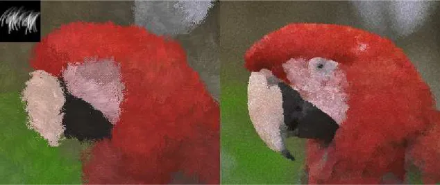
fully stochastic painting using rectangular strokes. Top: rst step (after rst layer), bottom: last step (nal painted image). . . 15 2.3 Samples of images used during tests (top-to-bottom: buttery, parrot, car, theatre,

airplane, lena, red ower). . . 16 2.4 Some examples of user-dened stroke templates. . . 17 2.5 Sample painted image using stroke style as shown in the upper left corner. Left

image: after rst step, right: last step. . . 18 2.6 Coarse painting with rectangular (left), uy (middle) and large circular (right)

stroke. . . 18 2.7 Sample painted by starting with the rst of the two templates shown, and nished

with the second one. . . 19 2.8 Area covered partially (left), then morphed (right). . . 20 2.9 Sample of painted image by using interpolative layer lling (only70%of the canvas

is covered) and edge following stroke orientation. a: model image, b: used edge map, c: rst layer, d: rst layer morphed, e: middle step, f : nal painted image. . 20 2.10 Sample for image painted with combination of edge following stroke orientation and

layer lling. . . 21 2.11 PSNR similarities (see equation 2.1) of painted image plotted against placed stroke

numbers (and a magnication of relevant areas): rendering with dierent stroke sets (decreasing from 1 to 10), while morph70 is 3-layer painting combined with interpolative layer lling (with70%coverage). . . 22 2.12 Transformation times and PSNR at the5000placed strokes point from Figure 2.11.

Using2-3layers give better transformation times at the same quality (compared to using more layers). . . 23 2.13 Some more examples for painted image quality (vertical) plotted against stroke

numbers (horizontal). . . 23 2.14 Stochastic 10-layer painting compared to enhanced painting with edge following

and layer lling. It is shown (for consecutive frames of the Mother and Daughter standard test video) that for achieving similar quality the new method is much faster. 24

III

(10)

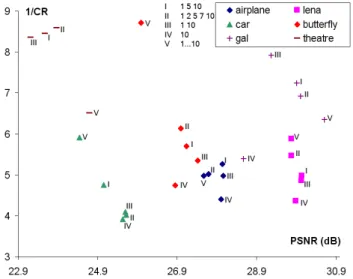
2.15 Rendering of6 dierent images, all with5 dierent runs with dierent stroke scales (labeled by roman numbers), plotting compression ratios (CR) against PSNR (see equation 2.1). Points show the positions where the rendering processes converged to. Sample images in Figure 2.3. . . 25 2.16 Detailed runs for the buttery image from Figure 2.15, plotting render times and

compression ratios (CR) against PSNR (see equation 2.1). With a selected goal e.g.

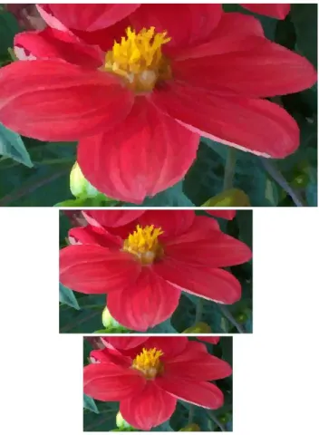
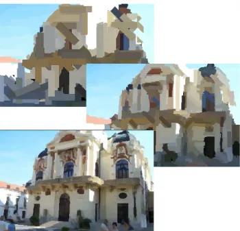
given quality in the shortest time one can select the appropriate rendering mode and vice versa. . . 26 2.17 Sample showing scalability. The images are all displayed from the same painted

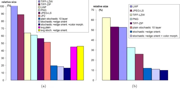
stroke-stream. . . 27 2.18 Sample for a painterly rendered image displayed from SVG format. . . 28 2.19 Comparing lossless compression rates of two example rendered image bitmaps by

dierent codecs and by stroke-stream compressions. Subgure a) also contains stored in SVG format (last 2 columns). . . 29 2.20 Lossless coding ratios of output stroke-series relative to lossless coded bitmaps of

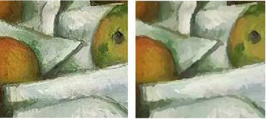
painted images. . . 30 2.21 JPEG coded oil painting segment (left) and the JPEG recoded with Paintbrush

rendering (right) - showing the ability to mimic stroke styles and noise ltering eects. 30 3.1 Extending stochastic painting to be controlled by internal image structure improves

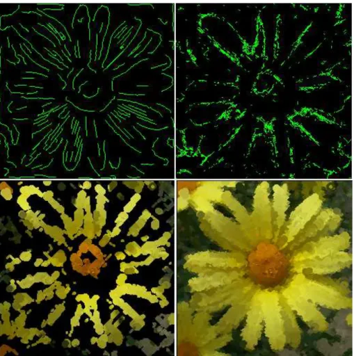
eciency: same PSNR quality (in this case 27.7dB for the Lena image and 28dB for the ower image in Figure 2.3) can be achieved in about half the time as fully stochastic painting requires. . . 37 3.2 Sample of painted image with the multiscale edge/ridge extraction based one layer

sequential painterly rendering model. Top: edge map and ridge map used, bottom:

rst step, and after closing the holes. . . 39 3.3 Example of image painted following edge orientations (random stroke positions,

sequential 10 layer stroke scales). . . 40 3.4 "normal" is the fully stochastic painting method with 10 layers, "eSPT" is the new

method with random stroke positions but following edge orientations when placing the strokes. It shows (for consecutive frames of the Mother and Son qcif video) that for achieving similar PSNR the new method needs much less time. . . 40 3.5 Example of image painted following edge orientation and scaling by ridge scales

(with random stroke positions). . . 41 3.6 Main steps of the 3rd painting approach. . . 42 3.7 Example of image painted following edge orientations, scales determined from ridge

scales, stroke positions are sequential. . . 43 3.8 Examples of image painted following edge orientations, scales determined from ridge

scales, stroke positions are sequential. On a) the main edge contours are also overlaid. 43 4.1 Example for an extracted relative focus map (left: input, middle: a coarse 2D map,

right: a corresponding class map). . . 46 IV

(11)

4.2 Steps of the iteration. . . 48 4.3 Error curves for8neighboring blocks (each curve stands for one block) on a blurred

texture sample (top) for the same blur with ADE (left), and MSE (right) . Ideally, curves of the same measure should remain close to each other. . . 50 4.4 Comparison of a) input image's b) MSE distance based extraction), c) PSF-based

classication and d) the new angle deviation error metric. . . 51 4.5 Example for focus map extraction with contrast weighting. a) input, b) focus map

without contrast weighting, c) focus map with contrast weighting and d) the extracted relative focus surface. . . 51 4.6 Example for extraction on the a) input image, with maps on the b) pixel level, c)

with overlapping blocks, and d) non-overlapping blocks. . . 52 4.7 Visual comparison for a) input image, for b) deconvolution, c) autocorrelation and

d) edge content based extractions. . . 53 4.8 Example images showing blurred texture discrimination properties of our (top right),

autocorrelation (lower left) and edge content based (lower right) methods. a) Top left is the input, numbers show increasingly blurred sub-areas. b) Top left is the input containing blurred areas shown with black borders. . . 54 4.9 Columns from left to right for each row: input image with a blurred area, decon-

volution based map, autocorrelation based map, edge content based map. Higher intensity means higher detected focusness. . . 54 4.10 Evaluation (lower is better) of the performance of deconvolution/ autocorrelation/

edge content extraction methods. For deconvolution both the new error measure (deconv) and the mean square error approach (deconv-mse) are investigated. Hori- zontal axis shows increasing blur, vertical axis shows extraction error relative to the real size of the blurred area. Blurred areas are shown with black borders. Errors larger than 100% mean that areas outside the ground truth area were also falsely detected as being blurred, thus increasing the error. . . 55 4.11 Examples for focus extraction on images with various textures (top row: input,

bottom row: respective focus maps). . . 56 4.12 Two examples of focus extraction on video frames: top row shows the video frames,

bottom row shows their respective focus maps (higher intensity means higher focus). 56 4.13 Following the move of focus across a scene (focus shifted from the left of the image

to the stairs in the background). Upper row are the input frames, bottom row are their respective focus maps with higher intensity meaning higher focus. . . 56 4.14 Map extraction results on some high depth of eld images. . . 57 4.15 Map extraction results on images with a focused area on blurred background. Columns

in each row from left to right: input, deconvolution based map, autocorrelation based map, edge content based map. . . 57 4.16 Samples for relative focus map extraction. Top: inputs and relative focus maps,

bottom: relative focus surfaces with four classes. . . 59

V

(12)

4.17 Sample image generation by lling the background layer with larger strokes and rening the foreground with smaller strokes. . . 60 4.18 Samples for color segmentation and cluster colorization. Left column: input, middle:

segmentation into 32classes, right: colorized clusters. . . 62 4.19 Sample generated image (from a to e): model, segmentation map for background

generation, colorized segmentation map, higher detail area, nal image. . . 63 4.20 Painted outputs. From left to right: input, and focus map; painted object on painted

background; painted on original; original on painted. . . 64 4.21 Rendering samples. Top: input images and their focus maps. Middle row: painted

objects on low-detail painted background. Bottom row: painted objects on segmentation- colorized background. . . 65 5.1 Cut detection used in the video painting process: cuts are detected by thresholding a

function which is a weighted product of edge and pixel dierence maps of consecutive frames. . . 69 5.2 Painting of videos: painted frame (a), motion eld extracted (b), generated frame

from previous frame and motion eld (c). . . 70 5.3 Encoding the painted frames as a stroke stream losslessly is more ecient than

encoding them as raster images with typical image coders in lossless mode.(eSPT stands for enhanced stochastic painting with edge following stroke orientations and layer lling, see Chapter 2). Numbers show average frame sizes for video samples. . 71 5.4 a) Variation of output size relative to uncompressed input avi size (in %) with

changing keyframe density (every nth frame is keyframe) for videos painted with dierent no. of stroke-sets. b) Relation between coding time and keyframe density for a sample video. . . 72 5.5 Using the enhanced painting process (eSPT) with layer lling and edge following

stroke orientations produces more stable frame sizes at the same quality which is better from the encoding point of view (normal stands for stochastic painting, eSPT stands for enhanced painting with edge following stroke orientation and layer lling). 72 5.6 Sample painted video frames. . . 73 5.7 Sample painted video frames. . . 73 5.8 Rendered oil painting (top:original) (Prole of a Woman / Zorka by József Rippl-

Rónai, 1916). . . 74 5.9 a) Rendered painting with uy template. b) Examples of painterly rendered images

(from top to bottom, top: model image, bottom: nal and comparison). . . 75 5.10 Examples of painterly rendered images (from top to bottom, top: model image,

bottom: nal) of real oil paintings. . . 76 5.11 MPVPlay, a test OpenGL painted image viewer. . . 77 5.12 Painterly rendered output as SVG, displayed in dierent sizes. . . 80 5.13 Storing the painted images as stroke series is more ecient than coding them with

image coders. . . 81 5.14 In many cases the SVG representation is shorter than the binary stroke sequence. . 81

VI

(13)

5.15 Some images used in the evaluation. . . 82 5.16 Viewing image rendered into SVG in a web browser. . . 82 5.17 Editing image rendered into SVG in Inkscape. . . 83 5.18 Left: SVG background formed from the buttery image. Right: The background is

formed from distinct color areas; some of them are here picked and placed to the side. 85 5.19 Left: the rened focus area with small strokes. Right: the fully painted image, the

rened area added to the background. . . 86 5.20 From left to right: downscaled model image; low detail background in SVG; rened

focus area with small strokes; nal rendered image. . . 86 5.21 Some examples of rendered images. . . 87 5.22 Query-response example. Left: the query and its map below, others: response

images and their maps. . . 89 5.23 Query-response example. Top-left: the query and its map; others: response images. 89 5.24 Precision-Recall graph for 10 dierent queries, in the case of a) the returned closest

10 matches and b) the use of a thresholded error measure for deconvolution- (deconv), autocorrelation- (AC) and edge content- (EC) based queries. The curves on the b) show values for a single query image for the 3 methods, given varying retrieval thresholds. . . 90

VII

(14)

List of Tables

1.1 Short feature list of referred methods. . . 9 2.1 Possible similar emulations of mentioned stroke representations by a common paint-

ing model (multiscale, template-based, stochastic) for using similar compression schemes. Last column shows approximations of bytes needed to store a stroke if simulated by the model. . . 32 6.1 Contributions by theses.. . . 93

VIII

(15)

1. Introduction 1

Chapter 1

Introduction

This rst chapter will be dedicated to an introduction of the eld of two dimensional non-photorealistic stroke-based rendering (NPR/SBR), basic techniques, methods and tools. A short historical background, the motivation behind this work, the goals and the steps towards achieving these goals will be presented. This work will be placed among the vast amount of achievements in the eld of NPR/SBR during approximately the last decade.

1.1 Context, goals, motivation

1.1.1 Context

Non-photorealistic rendering (NPR) techniques started emerging about a decade ago. Non-photorealistic is just what the name suggests - images created not with the goal to reproduce original imagery as close as possible, but to produce dierent representations of a model, something that might even be considered artistic. The rst goals of these techniques were to somehow imitate real life painting eects articially. Since the rst trials many dierent methods appeared, both in 2 and 3D, for many dierent purposes. Yet the rst goal has always remained: produce visually pleasant representations of model images or create such images articially with dedicated tools.

Non-photorealistic rendering has been used since then for many dierent purposes: to create painting-like eects on images, to produce cartoon-like renderings, to create dierent types of sketches, drawings, or even to aid the creation of illustrations from ordinary images (i.e. in medical imaging).

Stroke based rendering (SBR) methods form a special subset of non-photorealistic rendering

(16)

1.1.1. Context 2

techniques. In SBR the painterly eects are produced by simulating real life brush stroke to an extent, and the painting process itself, to produce images by a so called articial painting process.

Simulated brushes can be of a wide variety from simple geometrical shapes to multilevel height maps or complex curves.

As we will show later, there are many ways of generating painting-like images from ordinary pictures. The rough outline of these algorithms are as follows. We take an image that we wish to create a painterly rendered abstraction from, a model, and a blank image that we call canvas, on which we will create the painterly rendered image. The rendered image will consist of a series of brush strokes that will be placed on the canvas. The strokes can have dierent size, shape, orientation and color. These properties are the so-called stroke parameters which are the data needed to be known if we would wish to reconstruct the painted image later from the stroke-series it consists of. Strokes can be very versatile, and almost every researcher came up with their own version of the idea of a stroke. There are methods which use simple shapes (e.g. rectangles, lines, etc.) as strokes, others that use long curves with constant or varying width, then there are ones who use dierent templates or texture patterns as stroke models. The methods dier at most in the way they place the strokes on the canvas in order to obtain a plausible artistical representation of the model image.

There are manual, semi-automatic and fully automatic painting techniques. A manual painting method is a painting application, fully controlled by the user. Stroke sizes, positions, color, i.e.

everything is determined by the user. In manual painting approaches sometimes external haptic devices are also used to aid the artist in creating articial paintings. In semi-automatic painting techniques some parameters (for example stroke curve shapes or thickness) are determined by the user, but color/texture, lling and placing is done automatically. In automatic painting techniques the whole painting process is automatically controlled by the algorithm (sometimes parameters need to be set before starting the rendering process).

SBR algorithms can again be classied by a dierent property, into two main groups: greedy and optimization algorithms. Greedy algorithms usually consist of a method which tries to place strokes which locally or globally seem to improve the image on the canvas, with no or minimal consideration of stroke neighborhoods, stroke density or other parameters. Optimization algorithms usually contain some kind of built-in intelligence in the stroke placement and/or acceptance steps, which help the painting process converge faster or to converge more to some global minimum rather than to a local dead-end.

Usually the output of the rendering process is a series of stroke parameters, which can be

(17)

1.1.2. Goals 3

stored and later be used to reconstruct the painted images (and possibly also for other purposes as we will show later on).

1.1.2 Goals

Our work in the eld of NPR/SBR has been concentrated around 2D, model based SBR techniques.

The goals we pursued were to achieve automatic painterly eects on model images and videos, and at the same time to investigate dierent aspects of SBR like optimizations, coding, compression, scalability, etc.

Thus in our work and research in 2D SBR the source is a usual 2D image which is used as a model for the painting process. All data needed for the painterly transformation is obtained from this model image using dierent image analysis techniques. Our additions to the world of 2D SBR has been various, the most important probably having been a combined point of view not just from computer graphics but also from image processing and computer vision. This gave the opportunity to see dierent aspects of SBR besides the generation of painterly eects.

Also, we have to state that our goal has not been to produce painting or painter-aiding applications in which some real painter can create paintings by using simulated digital counterparts of real painters' tools, as in [5]. Our methods and techniques provide means to create painterly eects automatically, by using model images and stroke templates, without no user interaction.

Basically we have continuously targeted areas which have not been fully covered by graphics research in the eld of 2D SBR, mostly by combining techniques from image processing, pattern recognition and image coding. Thus, while we have been producing painterly eect generation methods, we always have also been dealing with storing, compressing and managing such produced images.

This thesis work presents most of our previous research in the eld and also some new achievements that are being published or being prepared for publication.

1.1.3 Motivation

The author's motivation in this work comes from the challenging, and widely unresolved tasks the 2D NPR/SBR techniques contain. As we will show in the next section, there are many NPR, and among them many 2D SBR methods. Some of them target specic application areas, like pencil or charcoal drawings, others try to simulate watercolor painting, there are ones that mimic oil paintings, of course there are many drawing-aiding applications which create an interactive

(18)

1.2. NPR/SBR Overview 4

painting environment for the users, and so on. Among these methods there are some, which try to produce (semi-)automatic painterly eect generators, which is also our target area.

These methods produce painting-like images in a wide variety of styles and ways, each having its pros and cons. Our motivation to work in this eld was to create fully automatic, and totally image structure and feature extraction based SBR methods. Of course other methods have also incorporated some image information to some extent during the rendering process, like edge or texture information, still, there were no methods which would base the control of the entire process on image features and remain fully automatic. This was one area which we targeted.

Another area which we tried to contribute to, was something which most of SBR techniques did not address: what should happen with the generated images, in what format and in what way should they be stored and handled ? Generally the produced images are stored as raster images, or video frames, or 3D meshes in the case of 3D NPR. This can cause a lot of problems, e.g. how should these images be scaled (scaling the raster images with interpolation methods, regenerating the painting into a dierent scale ?), how should they be compressed (since line, or stroke based renderings easily gain compression artifacts), how should the use for animations be handled, and so on. We tried to address these areas and investigated these issues.

1.2 NPR/SBR Overview

In [25] Haeberli introduced a simple interactive painterly rendering program. The technique was to follow the cursor, point sample the color and paint a brush stroke with that color. A stochastic process was responsible for putting the strokes on user-dened positions. Haeberli has also described a relaxation method for painting based on a kind of Voronoi algorithm. While the later algorithm is more automatic, it gives a quite synthetic result.

In Salisbury et al.'s [91] an interactive technique was introduced which produced high quality pen and ink type of contour-based sketches of model images. A similar silhouette painting algorithm is presented in Northrup et al.'s [79]. In [11] Curtis et al. created a watercolor paint system and demonstrated how computer-generated watercolor can be used as part of an interactive watercolor paint system, as a method for automatic image watercolorization, and as a mechanism for non- photorealistic rendering of three-dimensional scenes.

In Litwinowitcz's work [71] strokes with a given center, length, radius and orientation are generated, adding random perturbations and variation, gradient-based orientation. The author also uses stroke clipping for retaining edges and anti-aliasing. Hertzmann presented an algorithm [31]

(19)

which painted an image with a series of B-spline modeled strokes on a grid over the canvas.

The paintings were built in a series of layers, starting with a rough sketch then rened with smaller brushes where necessary. Later he implemented a back-end for rendering brush strokes [35]

produced by painterly rendering systems like this or like Meier's one described later. Hertzmann also extended his method to video processing [32].

In Szirányi et al.'s [104,105] the so-called Paintbrush Image Transformation was introduced, which was a simple random painting method using rectangular stroke templates, up to ten dif- ferent stroke scales in a coarse-to-ne way also for segmentation and classication purposes. A multiscale image decomposition method was presented, the resulting images of which looked like good quality paintings, with well dened contours. The image was described by the parameters of the consecutive paintbrush strokes. In Szirányi et al.'s [106] developments were presented, which included the usage of dynamic Monte Carlo Markov Chain optimization at the stroke acceptance step. Faster convergence was supported by a dynamic Metropolis Hastings rule.

In [45] Kaplan et al. presented an algorithm for rendering subdivision surface models of complex 3D scenes using an interactively editable particle system. Geograftals are used (special types of triangle strips), following the works of Meier [76] and Kowalski [63]. In [76] Meier used NPR techniques to create hand-paint like animations. 3D models and particle systems are used, a technique not really suited for 2D painterly processing.

An automatic painting system was introduced by Shiraishi et al. [96] The method generates rectangular brush strokes. Properties of strokes are obtained from moments of the color dierence images between the local source images and the stroke colors. The method controls the density of strokes as well as their painting order based on their sizes. The density is controlled by a dithering method with space-lling curves.

Hertzmann's other work [33] is a relaxation technique to produce painted imagery from images and video. He uses an energy function similar to the one used by the Paintbrush algorithm [104] by Szirányi et al. and minimize it in a quite sophisticated way (Hertzmann's implementation deletes, adds and relaxes the strokes, where the relaxation means the modication of some of the stroke parameters). Modifying this energy function, he is able to follow several painting styles.

In Szirányi et al.'s [105] the relation between painterly rendering and anisotropic diusion (AD) is suggested. Nonlinear partial dierential equations can be used for enhancing the main image structure. When compressing an image, AD, based on the scale-space paradigm, can enhance the basic image features to get visually better quality as Kopilovic et al. show in [48]. Determining the used stroke color based on blurring the underlying area and selecting the most recurring color

(20)

also shows some compatibility with AD because of its integrating nature.

Hertzmann et al. [34] introduced a method which can produce ltered images based on training images. They also use lters, e.g. they apply an anisotropic diusion or similar lter (a blurring lter) for preprocessing, in order to maintain good contours but eliminate texture. The goal of this work is to try to propagate a painting's style by painting images with stroke parameters extracted from another image.

In [29] Hays et al. present a still and motion picture painting method based on generating meshes of brush strokes with varying spatio-temporal properties. Strokes have location, color, angle and motion properties. By using textures and alpha masks they can mimic dierent styles.

Like in Kovács et al. [50], motion data is used to paint video frames, in this case for propagating the stroke objects along motion trajectories, which in some cases can lead to disturbing eects with strokes moving all over the video frames, giving a uid-like feel to the image. In Park et al.'s paper [81] a brush generation technique is presented where spline brush colors are obtained by generating a color palette from selected reference images, strokes follow image edge orientations, and stroke clipping at edges is also used.

In the work of Gooch et al. [24] a method was presented that produced a painting-like image composed of strokes. This approach extracts some image features, nds the approximate medial axis of these features, and uses the medial axis to guide brush stroke creation. In [43] Jodoin et al. present a hatching simulation stroke based rendering method, N-grams and texture synthesis tools to generate stroke patterns from a training stroke model and use the generated patterns to render 2D or 3D images and models in hatching style.

Santella and DeCarlo presented a method [15] which combines aspects from the approaches of Haeberli [25], Litwinowicz [71] and Hertzmann [31]. They extended their work with a system collecting eye-tracking data from a user in Santella et al.'s [92]. In their system they use curved strokes with single color and paint in details only the picture elements that attracted the user's gaze. We will present a method which has similar goals but does not need external devices, and will control the painting process by automatically estimated relative focus regions [58]. Mignotte in [77]

presents a sketching technique based on Bayesian inference and gradient vector eld distribution models combined with a stochastic optimization algorithm. The stroke model used is a B-spline with12control points pencil stroke.

In [110] Wang et al. presented a video transformation technique based on user performed segmentation on keyframes, interpolating of regions through frames and painterly rendering the segmented areas. Spatio-temporal surfaces are constructed from segmented areas over frames for

(21)

1.3. New scientic results in this work 7

smoothing using so called edge and stroke sheets.

The system in [44], by Kalnins et al., lets the designer directly annotate a 3D model with strokes, creating a subjective 3D NPR representation of a model object. The user chooses a brush style and draws strokes over the model from multiple viewpoints then the system adopts these strokes when rendering the scene to maintain the original look. Another system presented by Xu et al. in [109] is a semi-automatic painting system, where a user with a tablet and a pen can simulate painting eects, the brushes being 3D simulations of real brushes using pen pressure and orientation information to achieve more realistic representations.

1.3 New scientic results in this work

As we also have shown in the introduction, the stroke based rendering literature knows a fairly large number of methods and techniques for producing 2D painterly images. Most of these methods use image analysis results on some level of the rendering process. Our point of view and our methods dier from these approaches essentially since we have continuously concentrated on starting from and controlling the painting process by image structure information. That is, while the other methods incorporated image content information on some level, our methods are based on image content and structure analysis from the ground up. Another main dierence that our approaches brought is that we have not stopped at the output of a painterly rendering method, but investigated other possibilities, like storage, encoding and compressing possibilities of generated images, and also scalability and portability issues. We have developed new methods for automatic painterly eect generation, rst by extending stochastic painting, then by introducing scale-space feature controlled painting variations, by investigating optimal stroke set use multilayer painting, by introducing automatic focus based painting, and by various applications of these methods. We will detail the specic dierences and new additions in the respective chapters.

We have to clearly state here, that this work has its roots in the stochastic paintbrush transformation method of Szirányi et al. [105], which we shortly introduce in Chapter 2.1. All other parts of the present work are the author's own works and results.

Our publications in the eld include the following. In [49,50] we presented our rst steps in cartoon style transformation of image sequences based on painterly transformation of keyframes and optical ow based interframe post-painting. In these works a fairly simple stochastic painting process was used, generating the painted image by randomly placing dierent sizes of rectangular strokes to mimic the model images or video frames. Later starting from [51,52] more emphasis has

(22)

1.3. New scientic results in this work 8

been added to the coding and compression possibilities of painterly rendered images, showing that ecient lossless encoding can be done when storing the painted images as series of stroke parameters instead of raster images. In [54, 55] we investigated the applicability of painterly rendering in re- generation of original paintings, for storage and also for producing dierent reproductions by using various stroke templates and styles to generate other representation of real paintings. In [53] and later in [56] we presented methods combined with scale-space feature extraction where special weighted edge and ridge maps were used to control the painting process, producing a more natural rendering, with less layers. In [60] we proposed to render the paintings into scalable vector graphics (SVG) for more portability and ease of handling. In [61] we introduced a two-layer painterly rendering with location dependent detail control by using our automatic relative focus map extraction method [58].

Generally, comparing dierent stroke-based non-photorealistic rendering methods objec- tively is a seemingly impossible task. Given all the years of development in the eld, and given such broad surveys like Gooch & Gooch's [23], Strothotte et al.'s [100] or Hertzmann's [36], there is still no objective way to compare two NPR images. This is because of the really wide variety of subjective styles these methods produce, and the really broad range of simulation possibilities.

What we can do is comparing the methodologies used in generating a narrow class of NPR images, which in our case is automatic, image feature controlled stroke-based image generation. One approach are comparisons like Tables 1.1 and 2.1 try to show. Oftentimes, there are fairly minor dierences between the methods these renderings use still they can produce endless dierent styles.

Table 1.1 (at the end of this chapter) provides a comparison of our and related techniques based on criteria like stroke type, stroke representation or automatism abilities. Related approaches include related 2D SBR methods presented in the previous Overview section, those of Haberli [25], Litwinowicz [71], Curtis et al. [11], Hertzmann [31,33,34], Shiraishi et al. [96], Szirányi et al. [106], DeCarlo et al. [15], Gooch et al. [24] and our approaches [53, 54].

Also, the later referenced Table 2.1 (which is at the end of Chapter 2) contains details about the stroke types used in similar SBR methods, and details regarding how these stroke models could be also produced by using a template based multiscale rendering method. That is, to show that SBR methods like the ones we have been working on are dierent from similar methods, still, many other approaches could be simulated by them.

(23)

1.4. Outline 9

1.4 Outline

After the introductory role of this chapter, Chapter 2 will present detail on basic stroke based rendering by explaining stochastic painting and the various extensions, optimizations, coding and compression possibilities. Chapter 3 will present scale-space feature controlled painterly rendering.

Chapter 4 will present our recent relative focus map extraction technique and its applications in stroke based painting. Chapter 5 contains the presentation of various applications for the previously presented techniques. Chapter 6 has the conclusions followed by the bibliography and the thesis groups.

Ref. Stroke type Stroke Auto- Technique

representation matism

[25] geometrical color, orientation, partial draw an ordered list of geometrical strokes;

strokes size, shape, follow the cursor and point-sample the

position model then draw a stroke at that position [71] antialiased radius, length, full start at the center of a stroke and grow

lines clipped color, position, until edges are met then clip; randomly

at edges orientation perturb stroke parameters; orientation

following near-constant color [11] no strokes color chosen by partial trying to achieve watercolor style; ordered

the user, length, set of washes over a paper, position, orien- containing pigments structured into

tation glazes produced by uid simulation

[31] long curved B-spline control full use ne strokes only when necessary, strokes, points, brush size, painting layers of strokes upon each gradient based shape, color, other; place strokes on grid points style, orientation thickness,

parameters (8+)

[96] rectangular position, size, full start with larger and nish with smaller antialiased color, orientation strokes; orientation is based on image

strokes moments if the color dierence images

[33] short lines color/texture, partial strokes based on contour approximation opacity, shape, with dierent styles, controlled by

position, size, style energy functions

[34] no strokes, lter descriptors partial use lters to produce articial eects

ltering simulating the style of the model

[106] rectangular, position, orientation, full coarse-to-ne painting, starting with

or user color, size larger and rening with smaller strokes;

dened binary orientation determined by a stochastic rela-

bitmaps xation technique; MCMC optimization at

the stroke acceptance step [15] following line thickness, partial painting controlled by eye-movement

edge-chains, length, color curved strokes

[24] central axis of seg- control points of full stroke creation guided by approximate mented areas a B-spline (control feature medial axes; rendering: draw combined into; polygon); scalar parallel lines in the direction of

tokens Filbert brush polynom blending the stroke B-spline

simulation width values; color

[54] user-dened style, position, full coarse-to-ne stochastic placement of grayscale (256 orientation, stroke templates through multiple scales;

levels) templates color covering only certain percent of the canvas on a layer then use layer lling;

following and aligning to model edges [53] any shape and position, color, full model weighted edges control stroke

size of brush orientation orientation and weighted ridges control

templates grown stroke scale (meaning stroke line width

into lines with radius); only one layer of painting,

varying thickness sequential (one coverage then ll the holes)

Table 1.1: Short feature list of referred methods.

(24)

2. Stochastic painterly rendering 10

Chapter 2

Stochastic painterly rendering

This chapter presents our basic grounding rendering method that was extended with features and used as a starting point for further development. Thus an automatic, stochastic painting will be presented with details on how the method works and which image features it uses for generating the images. Also, representation, coding and compression of the painted images will be discussed.

Regarding the connections with older or similar stroke based rendering techniques, this chapter presents new or enhanced results.

First stochastic painting is described, which is where this work has started from. Later painting generation by using freeform stroke templates with grayscale height maps is presented, which is a new addition over previous techniques. It is new in the sense that in previous works, a stroke is either a simple geometrical shape, or it is the result of interactive physical stroke simulation, but here we use a solution that is in the middle: weighted freeform templates can be dened and used in the automatic painting process, thus we have the possibility to generate dierent styles of the same model. Thus the automatic eect generator can have more possibilities.

Then, a new mid-process layer interpolation technique is presented, which we used to call color morphology, which is an interpolative layer lling step. This is a fairly straightforward eight- directional color interpolation method, in order to speed up the generation of coarser layers during the painting process. This is accompanied by an edge following extension, which means that during the painting process the stroke orientations should follow the direction of the nearest edges. The latter technique has been used in the SBR literature, but it is important to introduce it in order to prepare the presentation of our later scale-space structure based painting method.

We also present new research results regarding the numbers of layers (or stroke scales) used

(25)

2.1. Stochastic painting 11

in multilayer painting methods, presenting our results which show that using a higher number of layers than three is usually a waste of time and resources since it cannot generate better results in any sense.

The last section of this chapter contains our results regarding a special eld of SBR, which has not been covered, or supercially treated by others, namely issues concerning the storage, compression and scalability aspects of painterly rendered images.

2.1 Stochastic painting

The basis of this work was a stochastic painting process [105], where the painted image was built by placing simple geometric stroke shapes with constant color on a virtual canvas until a desired eect was achieved. The strokes' positions were picked randomly over the canvas area, the color of the strokes was taken from the area of the stroke on the model image. Each stroke could have eight orientations as a multiples ofπ/8. Strokes could be of multiple sizes, each size called a stroke scale. These scales were grouped in stroke sets, and stroke sets used during the painting process were iteratively changed by decreasing order of their sizes. This is where we started from, seeking new possibilities for improvement and creating new techniques.

In the following we will introduce our 2D SBR model and show that it can be a comparable general basic model for most methods from the broad literature of SBR. The main steps of this (or such) an algorithm are in Algorithm 2.1, and also in Figure 2.1.

load input image;

initialize canvas;

while there are smaller strokes do repeat

select stroke position;

select stroke orientation;

sample stroke color;

place stroke;

until stroke set change is required ; switch to smaller stroke set;

end

Algorithm 2.1: Steps of the plain stochastic painting process.

In the above algorithm steps, a stroke set change is required when no improvement (over a threshold) can be made to the canvas with the current stroke scale. That makes the self control of the painting process quite unique since it does not follow strict rules as a stopping condition, but a relative dierence checking between consecutive steps. In the base algorithm, the dierence

(26)

Figure 2.1: Stochastic painting algorithm steps.

between the model and the painting is checked at specic intervals (originally after every 5000 placed strokes) by a measure function, which is responsible for stopping the painting process if a goal is achieved. The measure functions can be e.g.

• PSNR (Peak Signal to Noise Ratio) value related to the model, which should be above a threshold, where

P SN R= 20log10( max

√M SE) dB (2.1)

where MSE is the mean square error between two images.

• relative error functionFerr which is

Ferr= err_i−1−err_i

erri < ε (2.2)

which should be lower than a thresholdε, and whereerri is the mean square error between the current painted stage and the model andei−1is the same for the previous painted stage.

The convergence of the painting process is guaranteed since the process is stopped given

(27)

that a specic dB dierence is achieved or the relative change between two consecutive steps is smaller than a threshold.

Before the painting process starts, color sampling for the dierent possible stroke sizes is performed as a preprocessing step. This is done by convolving the model imagef with all possible stroke patterns with all possible orientations, for obtaining a blurred image series from which color sampling will be performed.

bj =f ∗sij (2.3)

wherei= 0...stroke set number andj= 0...7 the orientations, and the blurred series

sij =si0·



 cos¡_π

8 ·j¢

sin¡_π

8 ·j¢

−sin¡_π

8 ·j¢

cos¡_π

8·j¢



 (2.4)

wheresi0 is the horizontal template in each stroke set.

Convolution is done in Fourier space (by multiplying the FFT of the templates with the FFT of the model image) for less computation time, exploiting a very important property of the Fourier transform, that convolution is equivalent to multiplication in Fourier space:

f(x)∗s(x) =F⁻¹[F(ω)S(ω)] = Z

ζ∈R^N

f(x−ζ)s(ζ)dζ (2.5)

Later during the painting process color sampling will be performed using these pre-generated images: the most frequently occurring color (c) underneath the stroke (sij) at a certain position (x, y) is taken, which we call majority sampling:

c(sij, x, y) = argmax

t histsij,x,y(t) (2.6)

wherehistis the local histogram of colors under the area of the strokesij at location(x, y).

The parameters describing a stroke are the stroke's id (identies the template and the size), position, orientation and color. Positions are relative, telling the distance from the previous stroke.

A very important property is that the size (in bytes) of describing a stroke is always the same, regardless of the size or shape of the used stroke. This means that for higher quality more of the smaller strokes have to be used and the size of the painted output (compressed stroke stream) can increase dramatically. We have to take this in consideration when doing the transformations.

The output of the painting process is a series of stroke parameters, which are then used to store the painted image with a lossless compression scheme using Human compression [112].

(28)

2.1.1. Notes and starter ideas 14

Any other lossless statistical encoder could be used, we chose this because of simplicity and good performance.

Of course during the painting process a series of strokes can be even fully covered by following layers. These fully covered strokes are deleted from the stroke stream at a nal stroke-elimination step when we go over the strokes in a backward direction and check whether they are covered by other strokes on a higher hierarchical level of layers.

A sample of an image transformed using this technique is shown in Figure 2.2 (the model image is the ower from Figure 2.3.

While this technique may seem a bit rough, being stochastic and brute force in its nature, it also allows for a great freedom in the painting process. This means it can be fairly easily extended with relaxation and dierent optimization techniques (as in [106,108]) and other usable extensions can be easily added, as we will show later.

2.1.1 Notes and starter ideas

From the data in Table 1.1 (at the end of Chapter 1) one can realize that while stroke generation and placement methodologies can be quite dierent, stroke representation techniques do not dier that much. This means the main parameters of used strokes in dierent painterly rendering techniques are very similar. In most cases we need to store some stroke style data (e.g. template identication, lter description, etc.), position, orientation and color data, sometimes scale data. In some cases additional data can occur e.g. stroke width variation. When storing the used strokes as spline curves one stroke gets represented not by an identier-position-scale-orientation data quadruple, but with a series of oating point control points. The main idea is that essentially there is not much dierence in the stored data stream representing the painted image (which in our case is a coded stroke stream).

Respectively, many stroke shapes and styles can be simulated with other stroke styles and templates of other techniques. As an example long lines even with varying width can easily be substituted with a series of rectangular or similar longish types of stroke templates and converted.

This means that the later proposed coding and storage can be used for all other similar painting techniques as well. For a quick overview of possible stroke emulations see Table 2.1 (at the end of this chapter) which suggests possible simulations of other painting techniques by a common multiscale, template-based rendering method, which then could be represented and coded by a common stroke-series based compression scheme which we also use for our methods.

In its basic form, stochastic painting with rectangular simulated strokes can produce very

(29)

Figure 2.2: Sample of painted image (red ower, in Figure 2.3) with 10 layer coarse-to-ne fully stochastic painting using rectangular strokes. Top: rst step (after rst layer), bottom: last step (nal painted image).

high quality painterly rendered images, but the stochastic process involves slow computation, and an unpredictable time to complete the painting process. Thus rst we worked on achieving algorithmic speedup while trying to retain the basic properties of the stochastic painting technique.

(30)

Figure 2.3: Samples of images used during tests (top-to-bottom: buttery, parrot, car, theatre, airplane, lena, red ower).

We will present some techniques which improve the algorithm, reduce computation times, and later techniques that change the nature of the painting technique from stochastic to sequential at the same time providing a more natural way of painterly image representation and rendering. We also will provide data regarding the usability of stroke-series based compression for painterly rendered imagery.

To summarize the motivations behind improving the transforming the basic stochastic painting idea, while stochastic painting can produce nice eects, it still has its limitations: no consideration of image structure, use of at homogeneous strokes, hard to estimate transformation time, need for complex optimizations, post-processing steps. We sought to alleviate or overcome these limitations.

(31)

2.2. Painting with templates 17

2.2 Painting with templates

Rectangular simulated strokes, however easy to handle, did not prove to be enough and able to generate multiple styles of paintings. Thus, we introduced the ability to handle and use any type and kind of stroke shapes, by generating grayscale stroke templates with 256 gray scales, and use them as templates in the painting process. This way many dierent styles can be simulated and interesting pictures can be generated.

The stroke templates can be any type of grayscale sample. During the painting process, stroke placement will take place by rotating and shifting a stroke template over the canvas

sij=si0·



 cos¡_π

8 ·j¢

sin¡_π

8·j¢

−sin¡_π

8 ·j¢

cos¡_π

8 ·j¢



+



dx dy



 (2.7)

wheresij is a stroke from setiwith orientationj,si0is the base template of seti,(dx, dy)are the target stroke center coordinates. The grayscale values of the generated template will be used as they were a height map, i.e. after the overall color of the stroke will be obtained by the previously mentioned majority sampling process (eq. 2.6) and the color of the stroke will be weighted by the grayscale values that the stroke template consists of

csij,x,y(u, v) =csij,x,y(u, v)·w(u, v)·ξ (2.8) (u, v) being the position over the stroke area, w the stroke height map, ξ a constant. Thus the color of the placed stroke will vary over its area, depending on the local weight of the template.

This method will not reproduce the model image's texture, but this is not its goal either. It should just give us more free hand in producing interesting stroke templates to produce dierent painting eects.

For some examples see Figure 2.4. One can even vary the stroke templates during the painting process, thus e.g. starting with a large round stroke shape and nishing with a longish uy shape. Stroke style changes only mean a change of an identication byte in the generated stroke stream. For an example of painterly rendering with a dierent stroke than rectangular see Figure 2.5.

Figure 2.4: Some examples of user-dened stroke templates.

(32)

2.3. Extensions: layer lling, edges 18

Figure 2.5: Sample painted image using stroke style as shown in the upper left corner. Left image:

after rst step, right: last step.

Figure 2.6: Coarse painting with rectangular (left), uy (middle) and large circular (right) stroke.

2.3 Extensions: layer lling, edges

An extension we introduced to our painterly rendering process, which we used to call color morphology, which is a layer lling step based on weighted directional color interpolation, does the following: after a given percent of canvas coverage by a certain stroke layer the process is stopped and uncovered areas are lled by an eight directional distance weighted color interpolation method.

The next painting layer takes up from this color-lled stage and continues the painting process.

When using multiple layers and stroke scales, switching to a smaller stroke-set occurs when painting ("correcting") the present step does not cause improvement larger than a threshold. If we stop earlier, when a given percent of the canvas area is lled, complete the remaining areas with layer lling and use this lled canvas as a starting point for the next layer, it turns out that a

(33)

Figure 2.7: Sample painted by starting with the rst of the two templates shown, and nished with the second one.

lesser number of placed strokes is enough to complete the painting. This is mainly because there will be some areas where the interpolative layer lling produces enough color information that the area will not need further stroke renement.

From a point Cx,y we search in 8 directions (i= 0..7) for the rst occurring color Ci. The color at Cx,y will be the weighted average of the found colors, where the weights are inversely proportional to the distance of Ci. We norm the di weights so as the sum of weights will be 1. The steps of the interpolation are in Algorithm 2.2. A canvas that is covered50%with rectangular strokes then lled look like Figure 2.8. A sample image using layer lling and simple edge following stroke orientation can be seen in Figure 2.9.

Another extension we introduced is that strokes placed during the painting process shall not have their direction picked stochastically, but from the edge/gradient data of the model image. That means that when placing a stroke on the canvas, the orientation of the stroke will be

d=distances of the 8 nearest colored pixels fromCx,y; dc=color values of pixels at respective distance fromd; dsum=P₇

i=0d[i];

sd=dsorted in increasing order;

fori= 0...7do

m=position ofd[i]insd;

wi=sd[7−m]/dsum thei^th weight;

c_i =d_c[i]·w_i thei^thcolor element;

end Cx,y=P₇

i=0ci/P₇

i=0wi;

Algorithm 2.2: Steps of the interpolative layer lling extension.

(34)

Figure 2.8: Area covered partially (left), then morphed (right).

Figure 2.9: Sample of painted image by using interpolative layer lling (only70%of the canvas is covered) and edge following stroke orientation. a: model image, b: used edge map, c: rst layer, d: rst layer morphed, e: middle step, f : nal painted image.

determined from the direction of the nearest edge line. That is, from a stroke place candidate the nearest edge line is searched, its direction is calculated and assigned to the respective stroke.

(35)

2.4. Optimizing layers and stroke scales 21

This way the produced images will be more coherent, less errors will be introduced by mis-oriented strokes and thus less time will be spent on correcting such mistakes during the painting process.

Figure 2.10 shows an example for such generated image.

(a) Model and its edge map

(b) First, middle and nal steps from the rendering process

Figure 2.10: Sample for image painted with combination of edge following stroke orientation and layer lling.

2.4 Optimizing layers and stroke scales

We investigated the possibly optimal number of stroke layers for stochastic multilayer/multiresolu- tion painting. We wanted to determine that minimal number of stroke scales which could produce similar quality results as a higher number of layers. The purpose of this research was to reduce transformation time, to produce more compact coded stroke stream on the output and to gather some theoretical ideas about the possibility of stroke scale number reduction.

In the original stochastic painting we used a x number of ten scales of strokes for covering the canvas during the painting process. Soon the question arose whether we really needed strokes of so many dierent sizes for optimal coverage. Under "optimal" we mean the optimal compromise between stroke number, quality (dB dierence) and time. We conducted experiments concerning

(36)

transformation times and stroke stream compression ratio with dierent numbers of stroke-sets, and also compared the older painting method with our newer approaches. Tests were performed on multiple dierent sized color images. Figure 2.11 contains render runs for a sample image (similarity errors plotted against placed stroke number), showing that using2-3 stroke scales can produce just the same quality dB dierence as when painting with ten scales. The graph in Figure 2.12 shows time required to arrive to the5000 strokes point in Figure 2.11. It shows that at the same stroke count painting with2-3layers is much faster (all producing PSNR quality within0.5 dB). Figure 2.13 contains some more examples.

Figure 2.11: PSNR similarities (see equation 2.1) of painted image plotted against placed stroke numbers (and a magnication of relevant areas): rendering with dierent stroke sets (decreasing from 1 to 10), while morph70 is 3-layer painting combined with interpolative layer lling (with 70%coverage).

(37)

Figure 2.12: Transformation times and PSNR at the5000placed strokes point from Figure 2.11.

Using 2-3 layers give better transformation times at the same quality (compared to using more layers).

Figure 2.13: Some more examples for painted image quality (vertical) plotted against stroke numbers (horizontal).

Figure 2.14 shows (for frames of the Mother and Daughter standard test video, some frames also on Figure 5.6) the rendering time comparison between ten-layer stochastic painting and the extended version with layer lling and using edge orientation for stroke placement. The enhanced version achieves the same quality in less time.

Figures 2.15 and 2.16 provide more insight into the experiments concerning nding the

(38)

Figure 2.14: Stochastic 10-layer painting compared to enhanced painting with edge following and layer lling. It is shown (for consecutive frames of the Mother and Daughter standard test video) that for achieving similar quality the new method is much faster.

optimum between stroke scales, compression ratios and transformation times. First, render run data regarding PSNR quality (see equation 2.1) against compression ratio (abbreviated as CR) is presented in Figure 2.15 for multiple dierent images and5 dierent rendering for each image with dierent stroke scales (represented by the roman numbers). The points show the positions where the renders stopped using the relative error checking method. What we should see is that the renders using2-3scales (i.e. runs labeled III and I) are always near the optimum in each point cloud. For further details one of the images (buttery,768x512pixels,24bit color) was picked and more detailed renders were run using the same stroke scales, and stopped at0.5dB intervals. Data is shown in Figure 2.16 both for time and compression ratio data plotted against PSNR quality.

Renders using scales1-10(i.e. all the scales) and only10(the smallest scale) were included as extreme situations. This extremity clearly shows, as in the upper diagram the1-10run requires much more time at every step, on the lower diagram the 10-run produces much bigger code at every step. Therefore, if we discard these two we can clearly see that the 1−5−10 run (using stroke scales of1 : 60×15pixels,5 : 37×9pixels and 10 : 10×3pixels) always runs close to the optimum - high compression rate and shorter running time - curves on both the compression ratio and time diagrams.

Naturally, if the goal of the rendering process is to produce the most compact stroke-series code, the full 10-layer painting can be used, but knowing that it will take much more time. On the other hand, when time or compression is a lesser issue, using the smallest stroke can lead to the best quality. But on the average, for the same PSNR using 2-3 stroke scales is enough, and the advantage in transformation time can be quite signicant (see upper part in Figure 2.16). For example, when one wishes to obtain 25dB painted quality in the shortest time, one would choose