On the Boundedness of Discrete and
Continuous Volterra Equations with Control Applications
PhD Thesis
by
Essam Mohsen Abdelhameed Awwad
Supervisors: Professor Istv´ an Gy˝ ori Professor Ferenc Hartung
UNIVERSITY OF PANNONIA
Doctoral School of Information Science and Technology University of Pannonia
Veszpr´ em, Hungary
2013
ON THE BOUNDEDNESS OF DISCRETE AND CONTINUOUS VOLTERRA EQUATIONS WITH CONTROL APPLICATIONS
Thesis for obtaining a PhD degree in
the Doctoral School of Information Science and Technology of the University of Pannonia.
Written by:
Essam Mohsen Abdelhameed Awwad
Written in the Doctoral School of Information Science and Technology of the University of Pannonia.
Supervisors: Dr. Gy˝ori Istv´an and Dr. Hartung Ferenc
propose acceptance (yes / no) propose acceptance (yes / no)
(signature) (signature)
The candidate has achieved ... % in the comprehensive exam,
Veszpr´em, ...
Chairman of the Examination Committee As reviewer, I propose acceptance of the thesis:
Name of reviewer: ... ( yes / no)
...
(signature) Name of reviewer: ... ( yes / no)
...
(signature) The candidate has achieved ... % at the public discussion.
Veszpr´em, ...
Chairman of the Committee Grade of the PhD diploma ...
...
President of UCDH
Tartalmi kivonat
Az ´altalunk v´egzett munk´anak k´et f˝o motiv´aci´oja van. Az egyik, hogy a szab´alyoz´aselm´elet´eben sz´amos olyan egyenletet haszn´alnak, amelyek alkalmas transzform´aci´o ut´an folytonos id˝otarto- m´anyban Volterra integr´alegyenletek, m´ıg diszkr´et id˝otartom´any eset´en diszkr´et Volterra differen- ciaegyenlet alakj´aba ´ırhat´oak ´at. A m´asik motiv´aci´ot a szab´alyoz´aselm´eletben gyakran haszn´alt BIBO stabilit´as fogalma szolg´altatta, amely l´enyege hogy a rendszer korl´atos bemenetre korl´atos kimenettel v´alaszol. Azokban az esetekben amikor a szab´alyoz´as alapj´at szolg´altat´o matematikai egyenletek ´at´ırhat´ok Volterra egyenletek form´aj´aba, a BIBO stabilit´as teljes¨ul´ese egyen´ert´ek˝u lesz azzal, hogy a Volterra egyenletek megold´asai korl´atos f¨uggv´enyek.
Ertekez´´ es¨unkben a f˝o c´el olyan matematikai felt´etelek keres´ese, amelyek teljes¨ul´ese eset´en a folytonos v´altoz´oj´u Volterra integr´alegyenletek, illetve a diszkr´et idej˝u differenciaegyenletek megold´asai korl´atos f¨uggv´enyek. Az ´altalunk nyert ´uj matematikai ´all´ıt´asok ´altal´anos´ıtanak, il- letve ¨osszefoglalnak sz´amos, az irodalomban ismert eredm´enyt. Vizsg´alataink vil´agosan r´amutat- nak arra, hogy l´enyegi k¨ul¨onbs´egek vannak a szab´alyoz´asban szerepl˝o nemline´aris tagok sze- rint. Nevezetesen, a megold´asok korl´atoss´aga er˝osen f¨ugg att´ol, hogy szuperline´aris, line´aris vagy szubline´aris-e a rendszer¨unk. Fontos kiemelni, hogy vizsg´alatainkban hangs´ulyt fektett¨unk a nem- linearit´as t´ıpus´anak, illetve a szab´alyoz´asban megjelen˝o id˝ok´eseltet´esek hat´as´anak vizsg´alat´ara.
A kapott matematikai eredm´enyek ´eless´eg´et, illetve bizonyos speci´alis esetekben a felt´eteleink sz¨uks´egess´eg´et elm´eleti m´odszerekkel, illetve szimul´aci´os vizsg´alatokkal t´amasztottuk al´a.
Abstract
Our work is motivated by the observation that many models used in control theory can be transformed into a Volterra integral equation in the continuous case, and into a Volterra difference equation in the discrete case. Another motivation was the notion of the BIBO stability which is used frequently in engineering control. This notion of stability requires that the system responds to bounded input with bounded output. In the cases when the mathematical model can be rewritten as a Volterra equation, to obtain the BIBO stability we need to check that the solutions of the Volterra equation are bounded.
In our Thesis the main goal was to find sufficient conditions implying the boundedness of solutions of Volterra integral equations and Volterra difference equations. Our new results unify and extend many earlier results from the literature. Our investigations show that there are significant differences between the different type of nonlinearity of the model equation. Namely, the conditions for the boundedness depend on wether the nonlinearity is sub-linear, linear or super-linear. It is important to note that we investigated the role of the type of the nonlinearity and also the the size of the time delay. The sharpness of the results and in some cases the necessity of the conditions for boundedness was shown both theoretically and by using numerical simulations.
Acknowledgement
First and foremost, all praise is due to Allah, who gave me the opportunity, strength, and patience to carry out this work.
I have the pleasure to thank my supervisors Prof. Istv´ an Gy˝ ori and Prof.
Ferenc Hartung for guidance and very valuable support throughout my years as a PhD student in Hungary. I am grateful for them outstanding efforts which have made this Thesis possible.
I would like to thank the Director of the Doctoral School (Prof. Ferenc Friedler) for his help and support, also I have the pleasure to thank everyone in Department of Mathematics and everybody helped me in Hungary.
I would like to thank the reviewers for my home defence (Prof. Katalin Hangos and Dr. R¨ ost Gergely) for their valuable comments and suggestions that helped to improve my Thesis.
Many thanks for all my friends and colleagues in Veszpr´ em, Budapest and Debrecen, they played a very important role in my life.
The last, but the most important thanks to my family: my father, my mother, my wife, my daughters and my son for their love, also for keeping me in their prayers.
iv
Contents
Acknowledgement iv
1 Introduction 1
1.1 Background and motivation . . . 1
1.2 The structure and content of the Thesis . . . 2
1.3 Notations . . . 5
2 Theoretical Background 7 2.1 Basic notions in systems and control . . . 7
2.2 A scalar delay differential equation . . . 11
2.3 A scalar delay difference equation . . . 13
2.4 Review of basic theory for Volterra integral equations . . . 15
2.5 Review of basic theory for Volterra difference equations . . . 17
2.6 The relation between boundedness and stability of Volterra difference equations . . 18
2.7 Numerical approximation of delay equations . . . 19
3 Nonlinear Volterra Integral Equations with Delay 21 3.1 Nonlinear Volterra integral equations . . . 21
3.2 Main result . . . 23
3.3 Some special cases . . . 24
3.3.1 Sub-linear estimate . . . 24
3.3.2 Linear estimate . . . 26
3.3.3 Super-linear estimate . . . 26
3.4 Example . . . 27
4 BIBO Stability of Controlled Nonlinear Systems with Time Delay 29 4.1 System description and preliminaries . . . 29
4.2 Main results . . . 31
4.3 Convergence of the solutions. . . 38
4.4 Numerical examples . . . 39
5 Boundedness of Solutions of Nonlinear Volterra Difference Equations with Constant Delay 46 5.1 Nonlinear Volterra difference equations . . . 46
5.2 Some definitions and remarks . . . 47
5.3 Main result . . . 48
5.4 Special cases . . . 49
5.4.1 Sub-linear case . . . 49 v
Contents vi
5.4.2 Linear case . . . 51
5.4.3 Super-linear case . . . 52
5.5 Some corollaries with convolution estimations . . . 53
5.6 The linear convolution with infinite delay . . . 56
5.7 Examples . . . 58
6 BIBO Stability of Difference Equations 63 6.1 Problem statement . . . 63
6.2 Main results . . . 65
7 Applications 73 7.1 El Ni˜no and the delayed action oscillator. . . 73
7.2 Numerical solutions . . . 76
7.3 A delay system of population model . . . 78
8 Conclusion 82 8.1 New scientific results . . . 82
8.2 Publications and conference lectures . . . 83
8.2.1 Publications in refereed SCI journal . . . 83
8.2.2 Publication in refereed journal . . . 84
8.2.3 International conference presentations related to the Thesis . . . 84
Bibliography 85 Appendix A 94 A.1 Proofs of some results in Chapter 3 . . . 94
A.2 Proofs of some results in Chapter 4 . . . 97
A.3 Proofs of some results in Chapter 5 . . . 99
Chapter 1
Introduction
Volterra integral equations (VIEs) and Volterra difference equations (VDEs) with time delays are the mathematical model of many evolutionary problems with memory arising from physics, engineering, biology, chemistry and so on. For example they arise from control theory, population dynamics, mathematical epidemiology, economics and large classes of engineering applications.
1.1 Background and motivation
Differential and integral equations with time delays appear frequently as mathematical models in natural sciences, economics and engineering, and they are used to describe propagation and transport phenomena (see, e.g., [6,21,24,29,30,39,66,76,88]). In mathematical control theory and control engineering the time delay may appear in the control, since time is needed to sense information and to react to it (see [23, 63,75,89, 105, 117, 126, 127] and some references cited therein). The first control applications using time delays go back to the 30s [19, 20], and since that it is an extensively studied field (see, e.g., [21, 24, 93, 94, 126]). A challenging task is to determine how the solution behaves ast→ ∞ (see e.g. [5,6,53,90–92]).
The presence of the time delay in the model makes the mathematical investigations more difficult, since a solution of a delay differential equation lives in an infinite dimensional space (e.g. the space of continuous functions) contrary to the solution of ordinary differential equations (ODEs) whose solutions are elements of a finite dimensional space. Therefore more advanced mathematical techniques required for the study of delay equation than for ODEs.
Discrete dynamical systems with memory also appear frequently in engineering and scientific modeling. They may arise as a result of a numerical approximation of a continuous model, or many cases the nature of the application is discrete [2,11,37,54,79]. In general some questions (e.g. the existence and uniqueness of solutions) are obvious for discrete equations, but there are
1
Chapter1. Introduction 2 other qualitative questions (e.g. stability conditions) which are more challenging than the similar question for continuous equations (see, e.g., [54,70]).
VIEs and VDEs include a large class of continuous and discrete dynamical systems, e.g., delay differential or difference equations with finite or unbounded delays. Therefore, many models which appear in engineering and scientific applications fit to this general class of equations. In this work we are interested in a basic qualitative property of VIEs or VDEs, namely the boundedness of the solutions. It is an important question from both theoretical and the application point of view.
Besides the fact of the boundedness, it is also important in applications to obtain a good upper bound of the solution.
In this Thesis we focus on the study of boundedness of the solutions of VIEs and VDEs. This question was studied for convolution type VIEs by Lipovan [87], for linear VIEs by Burton [14,15].
There are several books and papers investigating the boundedness and stability of the solutions of several classes of VIEs (see e.g., [9,13,29,30,43,76,103,111,125] and some references cited therein). Boundedness of solutions, stability and other related questions for several classes of VDEs are studied in [5,32,33,38,53,55,56,70–72,90–92,97,117,121–123].
Time delays play an important role in control systems, since delay may appear when a system wants to measure or react to information. Stability or stabilization of a system is one of the central questions which is investigated in control theory. Delayed feedback control used in many engineering applications, see e.g., the delayed resonator [96]; stabilization of turning processes with delayed digital PD controller [81]; state feedback control with time delay in vibrating systems [105]; delayed state feedback due to device delay [80]; stabilizing helicopter rotor blades using delayed feedback [40, 74]; damping oscillation in power systems [77]; stabilization of various systems [41, 83, 101, 102]. In some cases the presence of the delayed feedback may stabilize an oscillatory system [1, 99]. Note that in many of the above applications state feedback is used instead of output feedback.
Because of its simplicity, the bounded input bounded output (BIBO) stability is widely in- vestigated. The sufficient conditions for BIBO stability of dynamic systems without delays are obtained in [119,120] by using Lyapunov function techniques. More recently many researchers have focused their interest on the BIBO stability of nonlinear discrete and continuous time con- trolled systems with or without delays [9,34,59, 73,84–86,113,118] and some references cited therein).
1.2 The structure and content of the Thesis
The structure of this Thesis is the following. In Chapter1we give a list of notations and acronyms we use in the rest of the Thesis. In Chapter2we give some basic background, known results and notions on the topics we will use in later chapters in our investigation.
Chapter1. Introduction 3 In Chapter3 we study a general class of nonlinear VIEs of the form
x(t) = Z t
0
f(t, s, x(·))ds+h(t), t≥0,
and present a sufficient condition which guarantees the boundedness of the solution (see Theorem 3.2.1below). Our method is based on a special inequality and a comparison technique. We show in Example 3.4.1 below that our method can be applied in a case when the known method of Burton [15] cannot be applied. We formulate sufficient conditions for the cases when the nonlinearity of the VIE has sub-linear, linear and super-linear estimates (see Theorems 3.3.1, 3.3.3and 3.3.4 below, respectively ). In a special class of VIEs we show that our conditions are not only sufficient, but also necessary (see Theorem3.3.2).
In Chapter4 we consider a continuous time nonlinear system with delay ( x(t) =˙ g(t, x(t−σ(t))) +u(t), t >0,
y(t) =Cx(t).
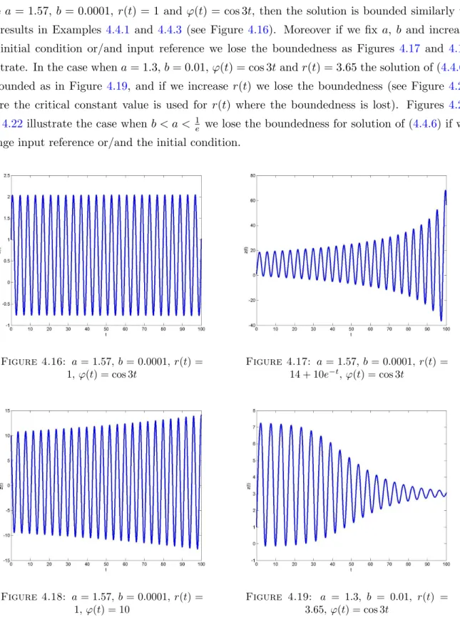
Here we propose a state feedback control law of the form u(t) =−Dx(t−τ) +r(t), where Dis a diagonal matrix, τ is a delay in the control mechanism, r is the reference input, to guarantee that the solution of the closed loop system is BIBO stable. We formulate sufficient conditions for the cases when the nonlinearity has sub-linear, linear and super-linear estimates, respectively (see Theorems4.2.1,4.2.3and4.2.6). In the super-linear case we prove a weak form of BIBO stability, which we call local BIBO stability. This new notion is introduced in Definition4.1.1. In practice it is useful if the delay in the control mechanism is relatively large. In our results we give a relation between D,τ and the bound of the nonlinear term which guarantees the BIBO stability of the nonlinear feedback control system. Our method is based on the variation of constant formula and the exponential estimate of the solution of the associated linear homogeneous delay system, and uses our general results on the boundedness of VIEs given in Chapter3. In some proofs we use the technique involving the integral of the absolute value of the fundamental solution of a homogeneous linear delay equation which was introduced in [47,50,51] in the study of stability of perturbed delay equations. The results of Chapter 3 and Chapter 4 on BIBO stability was published in [9]. In Section4.3we also give sufficient conditions in terms of the Lipschitz constant of the nonlinearity and the integral of the absolute value of the fundamental solution in the case of an autonomous nonlinear feedback control system (see Theorem4.3.1). The theoretical results are illustrated by several numerical examples (see Section4.4). Our numerical investigations show that our sufficient conditions give a good upper bound on the absolute value of the solutions. We also observe that in the case when the associated linear homogeneous equation has oscillatory solutions (the case when the delay is ”large” in the control mechanism) the solutions of the nonlinear feedback control system are also oscillatory.
Chapter1. Introduction 4 In Chapter 5 we give a sufficient condition to guarantee the boundedness of solutions of a general class of VDEs of the form
x(n+ 1) =
n
X
j=0
f(n, j, x(j−σ(j))) +h(n), n≥0.
Our main result of this chapter is formulated in Theorem 5.3.1. The results of this chapter are the discrete versions of those of Chapter3for VIEs. We also present special sufficient conditions for the cases of sub-linear, linear and super-linear nonlinearities (see Theorems 5.4.1, 5.4.5 and 5.4.7). We also discuss several special scalar VDEs in this chapter, and at some cases we obtain necessary and sufficient conditions (see Theorems5.4.3and 5.6.1and Corollaries 5.5.3-5.5.8). In Section 5.7we give several illustrative examples for the applicability of our results. The results given in this chapter are analogous with those of Chapter3, and they are extension of our earlier work [49] where an ordinary VDEs (without time delay) was investigated.
In Chapter6 we study a discrete time nonlinear system with time delay x(n+ 1)−x(n) =g(n, x(n−σ(n))) +u(n), n≥0
y(n) =Cx(n), n≥0.
We give sufficient conditions for the BIBO stability of the closed loop system for the sub-linear and linear cases (see Theorems6.2.1and 6.2.2). The results are the discrete counterparts of the results of Chapter4 given for continuous time controlled systems.
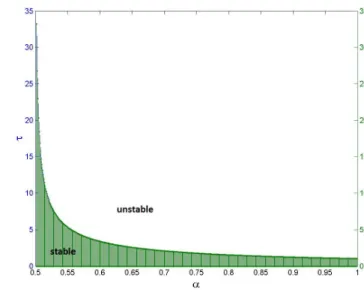
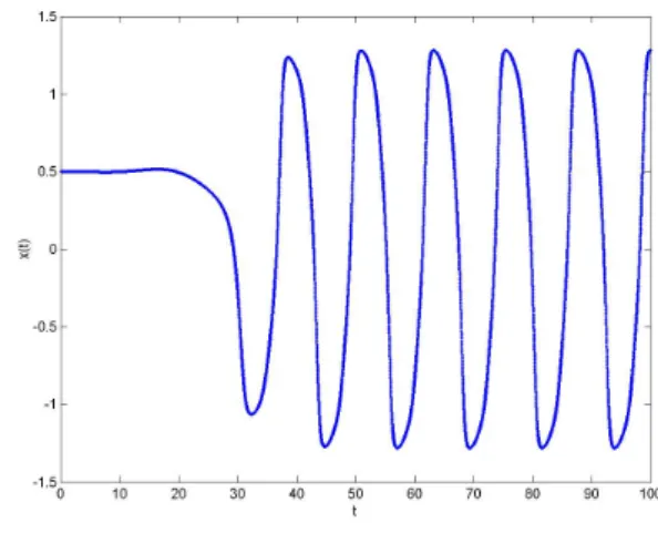
In Chapter 7 we present some applications of our results. First we discuss a model equation describing the El Ni˜no Southern Oscillation phenomenon observed in the equatorial Pacific. It is observed that there is a regular discrepancy of the see-level temperature of the ocean from the average temperature, and this anomaly shows a regular oscillatory behavior with a relatively large (about 1.5oC) amplitude. The mathematical model describing this temperature anomaly is investigated e.g. in [12,109]. In Section7.1we show that our method of Chapter3can be applied for this model, and we can give a sufficient condition which guarantees the boundedness of the solutions, moreover, for some cases the estimates of the upper bound of the solution obtained by our method gives a good approximation of the amplitudes of the oscillation in the solution of the nonlinear delay equation. Moreover, the oscillatory behavior of the associated linear homogeneous equation explains the appearance of the oscillatory solutions of the nonlinear equation for ”large”
delays. Numerical examples illustrate the theoretical results.
In Section 7.3 a class of population model equations is considered. This general model was introduced by Cooke and Kaplan [25], and later studied by many authors [17, 18, 46, 100].
In this section we show that we can find a control term of the form u(t) = ax(t) +r such that the corresponding closed-loop system has a unique, predefined equilibrium c, moreover, the solutions are bounded in a neighborhood of this equilibrium. This control term can be interpreted as a harvesting in the population proportional to the size of the population and a continuous
Chapter1. Introduction 5 immigration to the population with a constant rate. We show that the main method of Chapter 3 can be used to give a condition which implies the boundedness of the solution with initial population size close to the equilibrium for large classes of nonlinearities in the model equation.
In Chapter 8 we summarize the new results. Also the list of publications and conference lectures of E. Awwad related to the topic of this Thesis is given. Some technical or long proofs are moved to Appendix A.
1.3 Notations
The most important notations and acronyms used throughout in this Thesis are listed below in this section.
Mathematical notations
Z the set of integer numbers
N the set of nonnegative integers
C the set of complex numbers
R the set of real numbers
R+ the set of non-negative real numbers
Rd the space of d-dimensional real column vectors Rd1×d2 the space of all d1×d2 real matrices
xi ith element of vectorx
xT transpose of vectorx
Ld∞ the set of bounded functions R+→Rd
˙
x= dxdt time derivative of x
AT transpose of matrix A
diag{d1, . . . , dd} d×ddiagonal matrix with the elementsd1, . . . , dd in the main diagonal I the unit matrix of appropriate size I =diag{1, . . . ,1}
0 the zero matrix of appropriate size
k · k maximum normkxk:= max1≤i≤d|xi|of a vector x∈Rd
k · kτ the maximum norm of a continuous function x: [−τ,0]→Rddefined by kxkτ := max−τ≤t≤0kx(t)k
k · k∞ supremum norm of a function r∈Ld∞ defined bykrk∞:= supt≥0kr(t)k C(X, Y) the set of continuous functions mapping from X toY
S [−τ,0],Rd
the set of finite sequences {ψ:{−τ,−τ+ 1, . . . ,0} →Rd}, where τ ∈N kψkτ the norm of a sequenceψ∈S([−τ,0],Rd) is defined by
kψkτ := max−τ≤n≤0kψ(n)k.
Chapter1. Introduction 6 Acronyms
BIBO bounded input bounded output
EPCAs equations with piecewise constant arguments IVP initial value problem
LTI linear time invariant
ODEs ordinary differential equations VDEs Volterra difference equations VIEs Volterra integral equations
Chapter 2
Theoretical Background
In this chapter we review the most important concepts and known results which are used or referred to later in the thesis. Research works on control theory, feedback control, delay differential equations, delay difference equations, nonlinear VIEs, nonlinear VDEs, stability and boundedness on the solutions are reviewed.
2.1 Basic notions in systems and control
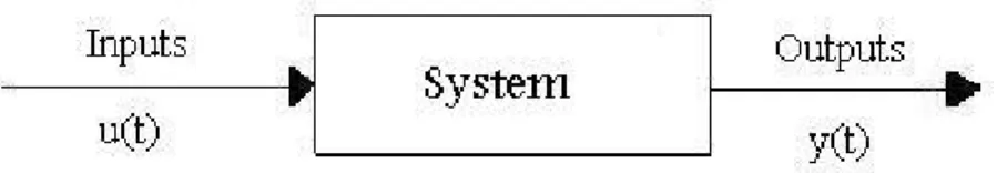
Control means to regulate, direct, command, or govern. A system is a collection, set, or arrange- ment of elements (subsystems). A control system is an interconnection of components forming a system configuration that will provide a desired system response. Hence, a control system is an arrangement of physical components connected or related in such a manner as to command, regulate, direct, or govern itself or another system. A control system provides an output as shown in Figure 2.1.
Figure 2.1: Description of a control system
Nonlinear systems
Any system which does not obey superposition principle is said to be a nonlinear system. Physical systems are in general nonlinear and analysis of such systems is complicated.
7
Chapter2. Theoretical Background 8 A general class of systems can be represented by the following state space model
˙
x(t) =f(x(t), u(t)), t≥t0
y(t) =h(x(t)),
(2.1.1)
wherex(t0) =x0andf :Rd×Rd1 →Rd,h:Rd→Rd2are nonlinear functions for positive integers d,d1,d2. The system or state model (2.1.1) is called time-invariant because the functionsf and h do not depend explicitly on time t; there are more general time-varying systems where the functions do depend on time. The model consists of two functions: the functionf gives the rate of change of the state vector as a function of state x and input u, and the output function h gives the measured values as a function of state x. We can model many physical systems in this form by carefully choosing the state variables and the analysis of nonlinear systems needs more sophisticated methods (see [59,67,69,108,112]).
Linear time invariant (LTI) systems
For linear systems, the state model (2.1.1) takes the special form
˙
x(t) =Ax(t) +Bu(t) y(t) =Cx(t),
(2.1.2)
where x ∈ Rd, u ∈ Rd1, y ∈ Rd2, A ∈ Rd×d, B ∈ Rd×d1, C ∈ Rd2×d and d, d1, d2 are positive integers. If the time is regarded to be a continuous variablet∈R+ in the above system (2.1.2), then the representation is a continuous time. The other possibility is to choose the time set to be discrete which results in a discrete time system model (see [8,67,68,124]).
LTI systems form the basis for engineering design in many situations. They have the advantage that there is a rich and well-established theory for analysis and design of this class of systems.
The importance of LTI system models is twofold: a lot of nonlinear ODEs can be transformed to an LTI one with an appropriate control input function, giving rise to the application of linear controllers on the linearized model.
Feedback systems
In most cases the control aim is reached by using feedback, i.e. the output signal is fed back to the input through a subsystem called controller (see Figure2.3).
We can investigate systems without and with controllers.
Open Loop Systems: A system in which the output has no effect on the control action is known as an open loop system.
Closed Loop Systems: A system which maintains a prescribed relationship between the con- trolled variable and the reference input, and uses the difference between them as a signal to activate the control, is known as a feedback control system. The output or the controlled
Chapter2. Theoretical Background 9
Figure 2.2: Block diagram of an output feedback control system
variable is measured and compared with the reference input. Thus the controlled variable is continuously fed back and compared with the input signal.
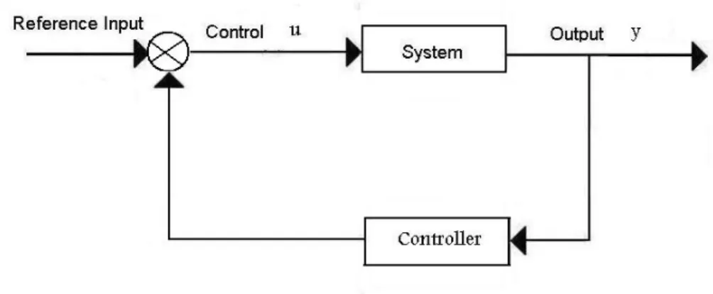
Feedback is a central notion in control theory, it is the property of a closed-loop system, which allows the output to be compared with the input to the system such that the appro- priate control action may be formed as some function of the input and output. In some cases we can measure the whole state, i.e., all components of the state. Then the structure of the controller can be a state feedback, which means, that the control input is determined as a function of the states
u(t) =k(x(t)), k:Rd→Rd1.
The linear state feedback law has the formu(t) =−Kx(t), whereK ∈Rd1×dis state gain matrix. In the case of affine state feedback Lawu(t) =−Kx(t) +r(t), whereK ∈Rd1×dis state gain matrix andr(t)∈Rd1 is the reference input (see Figure2.2).
Figure 2.3: Block diagram of state feedback control system
Output feedbacks use only output information to generate input, i.e., u(t) = ¯k(y(t)), ¯k:Rd2 →Rd1.
Chapter2. Theoretical Background 10 BIBO stability
Stability is a basic system property. There are various but related notions in systems and control theory to characterize the stability of a system. Internal or asymptotic stability is when the disturbance acts as an impulse and then the system behavior is analyzed when time goes to infinity, while external or BIBO stability describes the behavior of the system if it is subject to bounded but permanent disturbances.
There are different notions of BIBO stability. First consider the following definition.
Definition 2.1.1. [11, 59] A system is external or BIBO stable if for any bounded input it responds with a bounded output:
ku(t)k ≤M1 <∞=⇒ ky(t)k ≤M2 <∞, t∈[0,∞).
The following definition is asymptotic stability of LTI systems (see e.g., [11,59,93,117]).
Definition 2.1.2. The LTI system (2.1.2) is internally (asymptotically) stable if the solution x(t) of the equation
˙
x(t) =Ax(t), x(t0) =x0 6= 0, t≥t0 fulfills
t→∞lim x(t) = 0.
The following theorem from [11, 59] shows the relationship between BIBO and asymptotic stability in the case of LTI systems.
Theorem 2.1.3. Asymptotic stability implies BIBO stability for LTI systems.
Conversely, Perron’s theorem [98] yields that if the solutions of ˙x = Ax+u, x(0) = 0 are bounded for all bounded u = u(t), then all eigenvalues of A have negative real parts, i.e., the LTI system (2.1.2) is asymptotically stable. Note that this result was generalized for LTI systems with delay in [35,57].
An other version of the BIBO stability was introduced by Wu and Mizukami in [116].
Definition 2.1.4. The system (2.1.1) with state feedback law u(t) = −Kx(t) +r(t) is BIBO stable if there exist some positive constants θ1 and θ2 satisfying
ky(t)k ≤θ1krk∞+θ2, t≥0 for every reference inputr ∈Ld∞.
Chapter2. Theoretical Background 11 This is a stronger requirement compared to Definition2.1.1, since the constants θ1 and θ2 are independent of the reference input r. In the remaining part of the Thesis the notion of BIBO stability is used in the sense of Definition2.1.4.
In recent years, many researchers have focused their interest on the analysis of BIBO stability (see [34,59,73,113,118]) and BIBO stabilization (see [84–86,119,120]). We note that in most of the above papers the notion of BIBO stability is used in the sense of Definition2.1.4.
In Chapter 4 and Chapter 6 we investigate the BIBO stability of nonlinear continuous and discrete systems with delays respectively. To proof the BIBO stability we need some known results on delay differential equations, delay difference equations, VIEs, VDEs, boundedness of the solutions and stability.
2.2 A scalar delay differential equation
In this section we investigate a scalar delay differential equation which will be useful in Chapter 4. There are several works which give asymptotic stability of the solution for linear and nonlinear delay differential equations (see, e.g. [36, 39, 43, 47, 50, 51, 54, 58, 64, 76, 78, 106, 117] and references cited therein).
Consider the scalar nonlinear differential equation with constant delays
˙
x(t) =−ax(t−τ) +f(t, x(t−σ)), t≥0, (2.2.1) wherea >0,τ ≥0 and σ≥0 are given constants and the functionf :R→R is continuous and Lipschitz continuous. To obtain a (unique) solution of (2.2.1), we assume
x(t) =ψ(t), −%≤t≤0, where%:= max(τ, σ), andψ∈C([−%,0],R).
It is well known (see for example [36,43,47,51,54] ) that trivial solution of equation
˙
y(t) =−ay(t−τ), t≥0, (2.2.2)
is asymptotically stable if and only if 0< aτ < π2. We associate the initial condition
y(t) =ψ(t), −τ ≤t≤0 (2.2.3)
to (2.2.2), whereψ∈C([−τ,0],R). If 0< aτ < π2, then there exist positive constants (see Driver [36], p.325)M, and ¯α such that
|y(t)| ≤M e−¯αtkψkτ, t≥0.
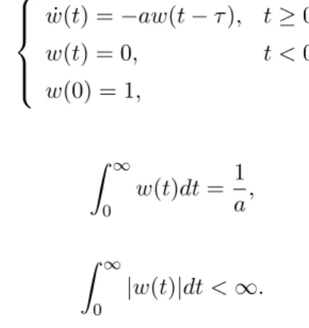
Chapter2. Theoretical Background 12 We also know (see e.g. [47,54]) that under condition 0< aτ <1/e, the solutionwof the IVP
˙
w(t) =−aw(t−τ), t≥0;
w(t) = 0, t <0;
w(0) = 1,
(2.2.4)
is positive and
Z ∞ 0
w(t)dt= 1 a, and if 0< aτ < π/2, we have
Z ∞ 0
|w(t)|dt <∞.
The solutionw(t) of (2.2.4) is called the fundamental solution of (2.2.2).
In the next figures we illustrate the above properties for the case when τ = 1 in (2.2.2). If 0 < a ≤ 1/e, then w > 0 and w converges to zero (see Figure 2.4). If 1e < a < π2 , then w is oscillatory but it is still convergent to zero (see Figure2.5). If a= π2 , then wis oscillatory and bounded (see Figure2.6). If a > π2 , thew is oscillatory and unbounded (see Figure2.7).
Figure 2.4: a= 0.35<1e Figure 2.5: 1e < a= 1.5< π2
Figure 2.6: a=π2 Figure 2.7: a= 1.58> π2
Chapter2. Theoretical Background 13 By the variation of constant formula [58] we get the solution of (2.2.1) as
x(t) =y(t) + Z t
0
w(t−s)f(s, x(s−σ))ds, t≥0,
wherey(t) is the solution of (2.2.2) and w(t) is the fundamental solution of (2.2.2).
Now we give the definitions of the stability and asymptotic stability. Let the solution of the IVP (2.2.2)-(2.2.3) be denoted by y(t, ψ).
Definition 2.2.1. The trivial solutiony= 0 of (2.2.2) is
(a) stable if for each >0 there is a δ >0 such that
kψkτ < δ implies |y(t, ψ)|< , t≥0.
Ify= 0 is not stable, then it is called unstable.
(b) asymptotically stable if it is stable and there is an η > 0 such that kψkτ < η implies
|y(t, ψ)| →0 as t→ ∞.
2.3 A scalar delay difference equation
In this section we give some known results on asymptotic behavior of solutions of linear and nonlinear scalar delay difference equations (see [7,37,44,47,50,51,54,65,82] and some references cited therein).
Consider the nonlinear scalar delay difference equation
x(n+ 1)−x(n) +λx(n−k) =f(n, x(n−`)), n≥0, (2.3.1) with initial condition
x(n) =ψ(n), −%≤n≤0,
where f is a continuous function, λ∈ (0,∞), k, ` ∈ N, % := max(k, `) and ψ ∈ S([−%,0],R).
The homogeneous linear equation corresponding to (2.3.1) is
y(n+ 1)−y(n) =−λy(n−k), n≥0, (2.3.2)
and the corresponding initial condition is
y(n) =ψ(n), −k≤n≤0.
The following is the definition of stability and asymptotic stability for discrete equation (2.3.2).
Chapter2. Theoretical Background 14 Definition 2.3.1. [2] The solutiony(n, ψ) = 0 is said to be
1. stable if, for each >0,there exists aδ=δ() such that, for any solutiony(n, ψ) of (2.3.2), the inequalitykψkk < δimplies ky(n, ψ)k< for all n≥0.
2. unstable if it is not stable.
3. asymptotically stable if it is stable and there exists a σ such that, for any solution y(n, ψ) of (2.3.2), the inequality kψkk < σimplies ky(n, ψ)k →0 as n→ ∞.
For the proof of our results later in this Chapter 6, we need the following lemmas which are based on the lemmas in [65].
Lemma 2.3.2. [65]Assume that k∈Nand
0< λ < kk
(k+ 1)k+1 (2.3.3)
holds. Then the unique solution {w(n)} of the IVP
w(n+ 1)−w(n) =−λw(n−k), n≥0;
w(n) = 0, −k≤n≤ −1;
w(0) = 1,
(2.3.4)
satisfies the following properties:
(a1) w(n)>0 for n≥0;
(a2) limn→∞w(n) = 0;
(a3) P∞
n=0w(n) = λ1.
The next lemma is the variation of constants formula for delay difference equations.
Lemma 2.3.3. [65]Let {x(n)} be the unique solution of (2.3.1) satisfying the initial condition x(n) =ϕ(n), −τ ≤n≤0,
where τ = max(k, `). Let {y(n)} be the unique solution of (2.3.2) satisfying the initial condition y(n) =ϕ(n), −k≤n≤0
and finally, let{w(n)} be the unique solution of the IVP (2.3.4). Then
x(n) =y(n) +
n−1
X
j=0
w(n−j−1)f(j, x(j−`)), n≥0. (2.3.5)
Chapter2. Theoretical Background 15 It is known (see e.g. in [70] and [82]) that the trivial solution of (2.3.2) is asymptotically stable if and only if
0< λ <2 cos kπ
2k+ 1
. (2.3.6)
Also for someM ≥0 and ρ∈(0,1) the solutiony of (2.3.2) satisfies the inequality
|y(n)| ≤M ρnkϕkk, n≥0, if condition (2.3.6) holds.
2.4 Review of basic theory for Volterra integral equations
The VIEs are a special type of integral equations and the mathematical model of many evolu- tionary problems with memory arising from physics, engineering, biology, chemistry and other sciences (see e.g., [13, 15, 29, 30, 103]). For example they arise in population dynamics, feed- back control theory, study of the behaviour of nuclear reactors and from the treatment of special hyperbolic differential equations.
The most standard form of linear VIEs is θ(t)x(t) =
Z t 0
k(t, s)x(s)ds+h(t), t≥0, (2.4.1)
wherek(t, s) is called the kernel of the integral equation (2.4.1), andh(t) is a continuous function of t. It is to be noted here that both the kernelk(t, s) and the function h(t) in equation (2.4.1) are given functions andx(t) is an unknown function that needs to be determined. If the function θ(t) = 0, then equation (2.4.1) simply becomes
h(t) =− Z t
0
k(t, s)x(s)ds, t≥0
and this equation is known as the VIE of the first kind; whereas ifθ(x) = 1, then equation (2.4.1) becomes
x(t) = Z t
0
k(t, s)x(s)ds+h(t), t≥0, (2.4.2)
which is called as the VIE of the second kind. Ifk(t, s) andh(t) are continuous, then there exists a unique solution of the VIE of the second kind. Equation (2.4.2) is said to be homogeneous if h(t) = 0 and nonhomogeneous otherwise. Also a homogeneous VIE of the second kind has only the trivial solution. Furthermore the kernelk(t, s) of an integral equation is called difference or convolution kernel if it depends only on the difference of the arguments,k(t, s) = ¯k(t−s).
In this Thesis in Chapter3, we focus our attention on the nonlinear VIE of the second kind:
x(t) = Z t
0
f(t, s, x(s))ds+h(t), t≥0, (2.4.3)
Chapter2. Theoretical Background 16 where x is a d vector, h : [0,∞) → Rd is continuous, and f : Ω×Rd → Rd is continuous with Ω ={(t, s) : 0≤s≤t <∞}. It is clear thatx(0) =h(0) in (2.4.3).
There has been interest in the literature over many years in studying the asymptotic behavior of the solutions of (2.4.3) and in particular, many results appeared on the existence and continuation of solutions of (2.4.3) and the convolution version of (2.4.3) (see, e.g., [15, 30, 45, 103], and references therein).
The boundedness of the solution of (2.4.3) and/or convolution case of (2.4.3) are investigated by Babolian and Shaerlar [10], Burton [15], Corduneanu [30], Lipovan [87] and other authors.
Proposition 2.4.1. [15] Let h be a continuous vector function on [0,∞) with |h(t)|< M, and suppose that k(t, s) is an n×n matrix continuous for 0< s < t <∞. If there existsm <1 with Rt
0|k(t, s)|ds < m for 0< t <∞,then all solutions of x(t) =h(t) +
Z t 0
k(t, s)x(s)ds are bounded.
Lipovan [87] has investigated the boundedness of the solutions of nonlinear VIE in convolution case
xp(t) =L(t) + Z t
0
P(t−s)x(s)ds, t≥0, (2.4.4)
wherep >1 is a constant,L∈C(R+,(0,∞)), P ∈C(R+, R+) and P 6= 0.
Theorem 2.4.2. [87]The solution to (2.4.4) is bounded if and only if the function L is bounded and
Z ∞ 0
P(s)ds <∞.
We remark that by the new variable y(t) =xp we can rewrite (2.4.4) in an equivalent form y(t) =L(t) +
Z t 0
P(t−s)y1p(s)ds, t≥0. (2.4.5) In Chapter 3, we consider a more general form of equation (2.4.5) ( see equations (3.1.1) and (3.3.2)) and we generalize and improve Proposition2.4.1and another results. We prove our results by new methods independent of Lyapunov function, Gronwall inequality, Lipschitz condition and resolvent kernel. Also we give sufficient condition to get the convergence of the solution of nonlinear integral equations with delay by using Banach fixed point theorem.
Chapter2. Theoretical Background 17
2.5 Review of basic theory for Volterra difference equations
We consider the nonlinear VDE
x(n+ 1) =h(n) +
n
X
j=0
f(n, j, x(j)), n≥0, (2.5.1)
whereh :Z→ Rand f :N×N×R→ Rare discrete functions. This equation can be regarded as the discrete analogue of the classical VIE of the second kind,
x(t) = ˜h(t) + Z t
0
f˜(t, s, x(s))ds, t≥0.
If we putf(n, j, x) =K(n−j)x we obtain the linear convolution case of (2.5.1) x(n+ 1) =h(n) +
n
X
j=0
K(n−j)x(j), n≥0. (2.5.2)
VDEs mainly arise in the modeling process of some real phenomena or by applying a numerical method to a VIEs or integro-differential equations. Stability, boundedness, and periodicity are among the most important properties of the solution of VDEs.
In recent years, there has been an increasing interest in the study of the asymptotic behavior of the solutions of both convolution and non-convolution-type linear and nonlinear VDEs (see [2,5,22,33,37,38,42,53,55,56,71,72,90,92,97,122,123] and references therein).
The boundedness and estimates of the solutions of discrete Volterra equations was investigated, (see e.g., [32, 49, 55, 71, 72, 97, 121] and references therein). Crisci et. al. ([32], Theorem 4.6) studied the boundedness of the solutions of VDE of a convolution system
y(n+ 1) =
n
X
j=0
H(n−j)y(j) + h(n), n≥0,
whereH is a matrixd×d,y(n)∈Rd,h(n)∈Rd andn≥0, under conditions
∞
X
n=0
kH(n)k<1, and kh(n)k< c, c >0.
Appleby, Gy˝ori, and Reynolds [5], under appropriate assumptions, proved the convergence of the solutions to a finite limit, which in general is non-trivial to the solutions of the discrete linear Volterra equation
x(n+ 1) =
n
X
j=0
H(n, j)x(j) + h(n), n≥0, (2.5.3)
Chapter2. Theoretical Background 18 with the initial condition
x(0) =x0, (2.5.4)
wherex(0) =x0∈Rd,H(n, j)∈Rd×d, 0≤j≤nand h(n)∈Rd.
The main result on the boundedness of solutions of (2.5.3) in [5] was improved by Gy˝ori and Horv´ath [53]. In terms of the kernel of a linear system Gy˝ori and Reynolds [55] found necessary conditions for the solutions to be bounded. Gy˝ori and Reynolds [56] studied some connections between results obtained in [5, 53]. Elaydi et al. [38] have shown that under certain conditions there is a one-to-one correspondence between bounded solutions of linear VDEs with infinite delay and its perturbation. Also Cuevas and Pinto [33] have shown that under certain conditions there is a one to one correspondence between weighted bounded solutions of a linear VDEs with unbounded delay and its perturbation. In most of our references linear and perturbed linear equations are investigated, moreover the boundedness and estimation of the solutions are founded by using the resolvent of the equations.
The following lemma is extracted from Appleby, Gy˝ori and Reynolds ([5], Lemma 5.3) and it will be needed in proof of Theorem5.4.5later.
Lemma 2.5.1. For every integerN >0,there exists a nonnegative constantK1(N) independent of the sequence (h(n))n≥0 and x(0) = x0, such that the solution (x(n))n≥0 of (2.5.3)-(2.5.4), satisfies
kx(n)k ≤K1(N)
0≤m≤Nmax kh(m)k+kx0k
, 0≤n≤N. (2.5.5)
Gy˝ori and Reynolds (2009) [55] found necessary conditions in terms ofHfor every solution of (2.5.3) to be bounded, but whenh(n) = 0 for alln.
2.6 The relation between boundedness and stability of Volterra difference equations
In this section we investigate relations between boundedness and stability for the solution of some VDEs. This problem is discussed by many authors (see, e.g., [2,32,79,91]). In general, there is no connection between boundedness and the stability of a solution of VDE. But, in the particular case of linear homogeneous equations, boundedness is equivalent to stability.
Now we consider the homogeneous linear Volterra difference system z(n+ 1) =
n
X
j=0
H(n, j)z(j), n≥0 (2.6.1)
whereH(n, j)∈Rd×d,z(j)∈Rdand 0≤j≤n.
Chapter2. Theoretical Background 19 The following theorems from [32] give the relation between boundedness and stability in the particular case.
Theorem 2.6.1. [32] A necessary and sufficient condition for boundedness of system (2.6.1) is its stability.
Theorem 2.6.2. [32]Assume that (2.6.1) is asymptotically stable and inequality kH(n, j)k< M νn−j, ν ∈(0,1)
holds for some M >0. If kh(n)k ≤C then system (2.5.3) is bounded.
Medina [91] investigated boundedness and stability properties of some classes of discrete Volterra equations and he gave some results about the relation between boundedness and stability of solutions.
2.7 Numerical approximation of delay equations
In this section we investigate numerical approximation of differential equations using the class of delay differential equations with piecewise constant arguments (EPCAs). EPCAs include, as particular cases, impulsive delay differential equations and some equations of control theory, and numerical approximation of differential equations with discrete difference equations (see [48,52]).
We show the method for nonlinear delay equations of the form
˙
x(t) =f(t, x(t), x(t−τ)), t≥0, (2.7.1) with initial condition
x(t) =ϕ(t), −τ ≤t≤0. (2.7.2)
Leth >0 be a discretization parameter. We associate the following EPCA to the IVP (2.7.1)- (2.7.2)
˙
yh(t) =f([t/h]h, yh([t/h]h), yh([t/h]h−[τ /h]h)), t≥0 (2.7.3) and
yh(t) =ϕ(t), −τ ≤t≤0, (2.7.4)
where [·] denotes the greatest integer part function. The right-hand-side of (2.7.3) is constant on the intervals [kh,(k+ 1)h), so the solution of (2.7.3)-(2.7.4) is a continuous function which is linear in between the mesh points{kh:k∈N}. Define `:= [τ /h].
We integrate both sides of (2.7.3) from kh tot, Z t
kh
˙
yh(s)ds= Z t
kh
f([s/h]h, yh([s/h]h), yh([s/h]h−`h))ds,
Chapter2. Theoretical Background 20 wherekh≤t <(k+ 1)h. Using that the integrand on the right-hand-side is constant, we get
yh(t)−yh(kh) =f(kh, yh(kh), yh(kh−`h))(t−kh).
Now taking the limitt→(k+ 1)h from the left-hand, we have
yh((k+ 1)h)−yh(kh) =hf(kh, yh(kh), yh(kh−`h)).
Since yh is linear between the mesh points, the values a(k) = yh(kh) uniquely determine the solution. The sequence a(k) satisfies the difference equation
a(k+ 1) =a(k) +f(kh, a(k), a(k−`))·h, k= 0,1,2, . . . , a(−k) =ϕ(−kh), k= 0,1,2, . . . , −τ ≤kh≤0.
It was shown in [48,52] that
h→0lim|x(t)−yh(t)|= 0, t≥0.
EPCAs were introduced by Wiener [114] and Cooke and Wiener [26, 27]. For surveys of theory and applications of such equations we refer to [4,28,115]. An application of this type of approximation was given in [61, 62], where numerical schemes were defined for the problem of estimating unknown parameters in several classes of differential equations.
Chapter 3
Nonlinear Volterra Integral Equations with Delay
In this chapter we consider a class of VIEs with delays. We formulate sufficient conditions for the boundedness of the solutions. Our general results will be applied in Chapter4 to obtain BIBO stability of a controlled nonlinear system.
3.1 Nonlinear Volterra integral equations
We consider the nonlinear VIE with delay x(t) =
Z t 0
f(t, s, x(·))ds+h(t), t≥0, (3.1.1) with initial condition
x(t) =ψ(t), t∈[−˜t0,0], (3.1.2)
where ˜t0 ≥0 is fixed, and the following conditions are satisfied.
(A1) The function f :R+×R+×C [−˜t0,∞),Rd
→ Rd is a Volterra-type functional, i.e., f is continuous and f(t, s, x(·)) = f(t, s, y(·)) for all 0≤s≤t and x, y∈C [−t˜0,∞),Rd
if x(˜µ) =y(˜µ), −t˜0 ≤µ˜≤s.
(A2) For any 0≤s≤tand x∈C [−˜t0,∞),Rd ,
|fi(t, s, x(·))| ≤ki(t, s)φ( max
−˜t0≤θ≤s
||x(θ)||), i= 1, . . . , d
holds, where f = (f1, . . . , fd)T. Here ki : {(t, s) : 0 ≤ s ≤ t} → R+, i = 1, . . . , d, is continuous, andφ:R+→R+is a monotone nondecreasing mapping such thatφ(˜v)>0 for
˜
v >0,and φ(0) = 0.
21
Chapter3. Nonlinear VIEs with Delay 22 (A3) h:R+→Rd is continuous andh(t) = (h1(t), . . . , hd(t))T,t≥0.
(A4) ψ∈C [−˜t0,0],Rd .
The notationf(t, s, x(·)) may denote non-delayed ordinary terms like f(t, s, x(·)) =g(t, s, x(s)), 0≤s≤t,
or may contain dependence of f on past values of the function x(·). This dependence can be described by a single point delay term or the form
f(t, s, x(·)) =g(t, s, x(s−σ(s))), 0≤s≤t, or by several point delays
f(t, s, x(·)) =g(t, s, x(s), x(s−τ1(s)), . . . , x(s−τn(s))) 0≤s≤t.
Also, the notationf(t, s, x(·)) may denote distributed delays of the form f(t, s, x(·)) =g(t, s,
Z s s−τ
b(s, u)x(u)du), 0≤s≤t, or more general dependence of f on past values ofx(·).
The next definitions will be useful in the proofs of our results on VIEs in this chapter.
Definition 3.1.1. Let the functions φ and ki be defined by assumption (A2). We say that the nonnegative constant µhas property (PT) withT ≥0 if there isv≥µ, such that
φ(µ) Z T
0
ki(t, s)ds+φ(v) Z t
T
ki(t, s)ds+|hi(t)|< v, t≥T, i= 1, . . . , d (3.1.3) holds.
Definition 3.1.2. We say that initial function ψ∈C [−˜t0,0],Rd
belongs to the set S if there existsT ≥0 such that
µT := max
−˜t0≤t≤T
kx(t)k
has property (PT), wherex: [−˜t0,∞)→Rd is the solution of (3.1.1)-(3.1.2).
Chapter3. Nonlinear VIEs with Delay 23 Remark 3.1.3. If there exist aT ≥0 and two positive constantsµT andvsuch that (3.1.3) holds, then
IT : = max
1≤i≤dsup
t≥T
Z T 0
ki(t, s)ds <∞, (3.1.4)
JT : = max
1≤i≤dsup
t≥T
Z t T
ki(t, s)ds <∞, (3.1.5)
HT : = max
1≤i≤dsup
t≥T
|hi(t)|<∞. (3.1.6)
Conditions (3.1.4) and (3.1.5) are equivalent to J0 := max
1≤i≤dsup
t≥0
Z t 0
ki(t, s)ds <∞, (3.1.7)
and if T = 0 condition (3.1.6) becomes H0 := max
1≤i≤dsup
t≥0
|hi(t)|<∞. (3.1.8)
3.2 Main result
In this section we give a sufficient condition for the boundedness of the solution of (3.1.1).
Theorem 3.2.1. Let (A1)-(A4)be satisfied and the initial functionψbelongs to the setS. Then the solution x of (3.1.1)-(3.1.2) is bounded.
Proof. Since the initial function ψ belongs to the set S, by Definition 3.1.2 there exists T ≥ 0 such that µT := max−˜t
0≤t≤Tkx(t)khas property (PT), where x is the solution of (3.1.1)-(3.1.2).
From (3.1.1) we get x(t) =
Z T 0
f(t, s, x(·))ds+ Z t
T
f(t, s, x(·))ds+h(t), t≥T.
Hence (A2) yields fori= 1, . . . , d
|xi(t)| ≤ Z T
0
|fi(t, s, x(·))|ds+ Z t
T
|fi(t, s, x(·))|ds+|hi(t)|
≤ Z T
0
ki(t, s)φ( max
−˜t0≤˜µ≤T
kx(˜µ)k)ds+ Z t
T
ki(t, s)φ( max
−˜t0≤˜µ≤s
kx(˜µ)k)ds+|hi(t)|
≤φ(µT) Z T
0
ki(t, s)ds+ Z t
T
ki(t, s)φ( max
−˜t0≤˜µ≤s
kx(˜µ)k)ds+|hi(t)|, t≥T. (3.2.1) Letv≥µT be such that (3.1.3) holds with µ=µT. Then, in particular,
φ(µT) Z T
0
ki(T, s)ds+|hi(T)|< v, i= 1, . . . , d,
Chapter3. Nonlinear VIEs with Delay 24 so (3.2.1) witht=T implies |xi(T)|< v for all i= 1, . . . , d, hencekx(T)k< v.
Now we show that kx(t)k is bounded for all t > T. For sake of contradiction, assume that kx(t)kis an unbounded function. Since it is continuous andkx(T)k< v, there existst1 > T such thatkx(t1)k> v. Let ¯t:= inf{t > T :kx(t)k> v}. Then the continuity ofx and µT ≤v implies
−˜tmax0≤˜µ≤¯t
kx(˜µ)k=kx(¯t)k=v.
Therefore there exists isuch that |xi(¯t)|=v. Then from (3.2.1) with t= ¯t, the monotonicity of φand using thatµT has property (PT), we obtain
v=|xi(¯t)| ≤φ(µT) Z T
0
ki(¯t, s)ds+ Z ¯t
T
ki(¯t, s)φ( max
−˜t0≤˜µ≤s
kx(˜µ)k)ds+|hi(¯t)|
≤φ(µT) Z T
0
ki(¯t, s)ds+φ(v) Z ¯t
T
ki(¯t, s)ds+|hi(¯t)|
< v,
which is a contradiction. So the solutionx of (3.1.1) is bounded by v.
3.3 Some special cases
In this section, we give some applications of Theorem 3.2.1. Throughout this section we assume that the components of the nonlinear function f in (3.1.1) can be estimated by the function φ(t) =tp,t >0 with p >0 in (A2). There are three cases:
1. Sub-linear estimate 0< p <1;
2. Linear estimatep= 1;
3. Super-linear estimate p >1.
3.3.1 Sub-linear estimate
Our aim in this subsection is to establish a sufficient, and in a special case, a necessary and sufficient condition for the boundedness of all solutions of (3.1.1).
The next result provides a sufficient condition for the boundedness of the solutions of (3.1.1) in the sub-linear case.
Theorem 3.3.1. Let (A1)-(A4) be satisfied and φ(t) = tp, t ≥ 0, with a fixed p ∈ (0,1). If (3.1.7) and (3.1.8) hold, then all solutions of (3.1.1) are bounded.
Chapter3. Nonlinear VIEs with Delay 25 Proof. It follows from (3.1.7) and (3.1.8) that J0 < ∞ and H0 < ∞. Let ψ ∈ C [−˜t0,0],Rd
, and xbe the corresponding solution of (3.1.1)-(3.1.2). For µ0:= max−˜t
0≤t≤0kψ(t)k, there exists v≥µ0 large enough such that
vp−1J0+1
vH0 <1. (3.3.1)
Therefore
vpJ0+H0 < v.
By the definitions ofJ0 and H0, we get vp
Z t 0
ki(t, s)ds+|hi(t)| ≤vpJ0+H0< v t≥0, i= 1, . . . , d.
Hence by Definition 3.1.1, we obtain µ0 has property (P0) with T = 0. Since (A1)-(A4) are satisfied and µ0 has property (P0), then, by Theorem3.2.1, the solutionx of (3.1.1) is bounded.
We consider the scalar VIE x(t) =
Z t 0
k(t, s)xp(s−τ(s))ds+h(t), t≥0, (3.3.2) with initial condition
x(t) =ψ(t), t∈[−˜t0,0], (3.3.3)
where
(B) k:{(t, s) : 0≤s≤t} →R+ and h :R+→R+ are continuous, 0< p < 1,τ ∈C(R+,R+),
˜t0=−inft≥0{t−τ(t)}>0 is finite and ψ∈C [−˜t0,0],(0,∞) .
The condition (B) implies that the solutions of (3.3.2)-(3.3.3) are positive.
The following result provides a necessary and sufficient condition for the boundedness of the positive solutions of (3.3.2). The necessary part of the next theorem was motivated by a similar result of Lipovan [87] proved for convolution-type integral equation.
Theorem 3.3.2. Assume (B), lim inf
t→∞
Z t 0
k(t, s)ds+h(t)
>0, (3.3.4)
and Z t
0
k(t, s)ds+h(t)>0, t≥0. (3.3.5)
Then the solution of (3.3.2)-(3.3.3) is bounded for all ψ ∈ C [−˜t0,0],(0,∞)
, if and only if (3.1.7) and (3.1.8) are satisfied.
Chapter3. Nonlinear VIEs with Delay 26 See the proof in AppendixA.1 (page94).
3.3.2 Linear estimate
Our aim in this subsection is to obtain a sufficient condition for the boundedness of the solutions of a linear VIEs with time delay.
The following result gives a sufficient condition for the boundedness.
Theorem 3.3.3. Assume (A1)-(A4) are satisfied and φ(t) = t, t ≥ 0. Then all solutions of (3.1.1) are bounded, if for some T ≥0 one of the following conditions holds:
(i) (3.1.4) and (3.1.6) hold, and JT := max
1≤i≤dsup
t≥T
Z t T
ki(t, s)ds <1, i= 1, . . . , d. (3.3.6)
(ii) for all t≥T, i= 1, . . . , d, JT := max
1≤i≤dsup
t≥T
Z t T
ki(t, s)ds= 1,
Z t T
ki(t, s)ds <1
sup
t≥T
1−
Z t T
ki(t, s)ds
−1Z T 0
ki(t, s)ds <∞, (3.3.7) and
sup
t≥T
1−
Z t T
ki(t, s)ds −1
|hi(t)|<∞. (3.3.8)
The proof can be found in Appendix A.1(page 96).
3.3.3 Super-linear estimate
Our aim in this subsection is to obtain a sufficient condition for the boundedness in the super- linear case.
Theorem 3.3.4. Assume that conditions (A1)-(A4) are satisfied with φ(t) = tp, t > 0, where p > 1, (3.1.7), (3.1.8) hold, J0 >0 and let kψkt˜
0 := max−˜t0≤t≤0kψ(t)k. Then the solution x of (3.1.1)-(3.1.2) is bounded if one of the following conditions is satisfied
(i) kψkt˜
0 ≤
1 pJ0
p−11
andH0 < p−1p
1 pJ0
p−11
;
(ii) H0<kψk˜t
0−J0 kψk˜t
0
p
.
Chapter3. Nonlinear VIEs with Delay 27 Proof. Assume (3.1.7) and (3.1.8) are satisfied.
(i) Since kψk˜t
0 ≤
1 pJ0
p−11 and
H0 < p−1 p
1 pJ0
p−11
= 1
pJ0 p−11
−J0 1
pJ0 p−1p
,
thenv:=
1 pJ0
p−11
satisfies inequality
H0 < v−J0vp. (3.3.9)
(ii) Since H0 <kψk˜t
0−J0 kψkt˜
0
p
, v=kψkt˜
0 satisfies inequality (3.3.9).
Hence in both cases the condition (3.1.3) is satisfied with T = 0, therefore µ0 := kψk˜t
0 has property (P0). Then the conditions of Theorem3.2.1hold, so the solution of (3.1.1) is bounded.
3.4 Example
The next we give an example that illustrates the applicability of Theorem3.3.3 in a case when condition (ii) holds for a large enoughT.
Example 3.4.1. We consider the scalar VIE x(t) =
Z t
0
2
1−0.5e−2|t−ln 2|e−2(t−s)x(s)ds+ce−2t, t≥0.
Hereh(t) =ce−2t,c∈Rand k(t, s) = 1−0.5e−2|t−ln 2|2 e−2(t−s), ˜t0 = 0.
Clearly supt≥0|h(t)|=|c|<∞, and Z t
0
k(t, s)ds= Z t
0
2
1−0.5e−2|t−ln 2|e−2(t−s)ds= 1
1−0.5e−2|t−ln 2|(1−e−2t), hence
t→∞lim Z t
0
k(t, s)ds= 1.
LetT1:= ln 2, then
Z T1
0
k(T1, s)ds= 1 (1−0.5)
1−e−2 ln 2
= 3 2 >1.
This means that
sup
t≥0
Z t 0
k(t, s)ds=M >1,
Chapter3. Nonlinear VIEs with Delay 28 therefore conditions of Theorem 3.3.3do not hold withT = 0.
If we take T := ln 5, then we obtain Z t
T
k(t, s)ds= 1−25e−2t
1−2e−2t <1, t≥T and
sup
t≥T
Z t T
k(t, s)ds= 1.
Moreover
1− Z t
T
k(t, s)ds
−1Z T 0
k(t, s)ds= 24e−2t(1−2e−2t) 23e−2t(1−2e−2t) = 24
23, t≥T, and
1−
Z t T
k(t, s)ds −1
|h(t)|= (1−2e−2t)
23e−2t |c|e−2t< |c|
23, t≥T.
Then condition (ii) in Theorem3.3.3is satisfied with thisT, therefore x is bounded.
We note that Proposition 1.4.2 in [15] cannot be applied for this example, but our sufficient
conditions can be used.
Chapter 4
BIBO Stability of Controlled
Nonlinear Systems with Time Delay
Stability of a differential equation is a central question in engineering applications, especially in control theory. Many different concepts of stability has been investigated in the literature, e.g., stability of an equilibrium of the system, orbital stability of the system output trajectory, or structural stability of the system. Because of its simplicity and weakness, the notion of bounded- input bounded-output (BIBO) stability was extensively studied and used in control theory for different classes of dynamical systems (see, e.g., [9,11,34,73,84–86,104,113,117,118]).
In this chapter we study the BIBO stability of a system with time delays controlled by a delayed state feedback. To obtain BIBO stability we rewrite the control system as a VIE by variation of constant formula and we apply our results on the boundedness in Chapter 4. Also we introduce a new notion of BIBO stability, which we call local BIBO stability.
4.1 System description and preliminaries
We consider the nonlinear system with delays
( x(t) =˙ g(t, x(t−σ(t))) +u(t), t >0,
y(t) =Cx(t) (4.1.1)
where x(t), u(t) and y(t) are the state vector, control input and control output of the system, respectively, σ(t) ≥ 0 is a continuous function, C ∈ Rm×d is a real constant matrix and g : R+×Rd→Rdsatisfies
kg(s,x)k ≤˜ b(s)φ(kxk)˜ , s∈R+, x˜∈Rd, (4.1.2) whereb(s)>0 is a continuous function, φ:R+→R+ is a monotone nondecreasing mapping.
29