CORVINUS UNIVERSITY OF BUDAPEST
D
EPARTMENT OFM
ATHEMATICALE
CONOMICS ANDE
CONOMICA
NALYSIS Fövám tér 8., 1093 Budapest, Hungary Phone: (+36-1) 482-5541, 482-5155 Fax: (+36-1) 482-5029 Email of corresponding author: zsolt.darvas@uni-corvinus.huWebsite: http://web.uni-corvinus.hu/matkg
W ORKING P APER
2013 / 7
T HE E URO A REA ' S T IGHTROPE W ALK : D EBT AND C OMPETITIVENESS IN I TALY AND S PAIN
Zsolt Darvas
October 2013
The euro area's tightrope walk: debt and competitiveness in Italy and Spain Zsolt Darvas
October 2013
Abstract:
Competitiveness adjustment in struggling southern euro-area members requires persistently lower inflation than in major trading partners, but low inflation worsens public debt
sustainability. When average euro-area inflation undershoots the two percent target, the conflict between intra-euro relative price adjustment and debt sustainability is more severe.
In our baseline scenario, the projected public debt ratio reduction in Italy and Spain is too slow and does not meet the European fiscal rule. Debt projections are very sensitive to underlying assumptions and even small negative deviations from GDP growth, inflation and budget surplus assumptions can easilyresult in a runaway debt trajectory.
The case for a greater than five percent of GDP primary budget surplus is very weak. Beyond vitally important structural reforms, the top priority is to ensure that euro-area inflation does not undershoot the two percent target, which requires national policy actions and more accommodative monetary policy. The latter would weaken the euro exchange rate, thereby facilitating further intra-euro adjustment. More effective policies are needed to foster growth.
But if all else fails, the European Central Bank’s Outright Monetary Transactions could reduce borrowing costs.
Keywords: competitiveness adjustment; debt sustainability; euro area; inflation JEL codes: E31; H68
Zsolt Darvas (zsolt.darvas@uni-corvinus.hu) is Senior Fellow at Bruegel, Senior Research Fellow at the Centre for Economic and Regional Studies of the Hungarian Academy of Sciences, and Associate Professor at Corvinus University of Budapest. The author is grateful for comments and suggestions by Guntram B. Wolff, Francesco Papadia, Shahin Vallee, and participants at a Bruegel internal seminar, at the Bruegel-Italian Treasury workshop in Rome on 8 May 2013 and the 10th European Seminar of ELIAMEP in Nafplio on 5-6 July 2013. Giuseppe Daluiso provided excellent research assistance.
1. Introduction
Southern euro-area countries face a number of challenges, such as achieving sustainable public and private debt positions, sound banking systems and improved competitiveness in the midst of a deep economic contraction and high unemployment, which are also fuelled by major structural weaknesses.
The triple crises of balance of payments, banking and sovereign debt, and the consequent growth crisis, are highly interrelated1.
Notwithstanding these difficult conditions, major adjustments have been achieved – but much more is necessary. For example, Italy’s almost 5 percent of GDP structural primary budget surplus suggests that further fiscal consolidation may not be needed. But Italy’s real exchange rate has hardly corrected and the country’s export performance remains weak, factors that call for a major adjustment. Spain is in almost the opposite situation: there has been a significant fall in unit labour costs (ULC) and Spain's export performance has been outstanding since 2008, yet its large external debt necessitates further improvements in exports, and a major fiscal adjustment is also still ahead. In both countries, the large stock of public debt means the fiscal situation is vulnerable.
There are five major ways in which high debt ratios can be reduced: fiscal consolidation, fast economic growth, high inflation, financial repression2 and default (Reinhart and Rogoff, 2011). Of these, sudden inflation reduces the real value of outstanding debt, while a steady dose of inflation – if the real interest rate is reduced because of, for example, financial repression or other factors –
contributes to the lowering of the debt ratio. But in order to regain price competitiveness, which was generally lost in southern members of the euro area before the crisis, low inflation or even deflation would be needed.
Generally, lower expected inflation reduces nominal interest rates and vice versa, as noted by Erwin Fisher a century ago. But this basic economic law did not apply to intra-euro interest rate
developments during the euro's first decade, because euro-area members' nominal interest rates largely converged, while inflation developments were very different in different euro-area members.
And this law does not apply either to current intra-euro area divergences in interest rates. There is flight to safety and, because of the shortage of AAA assets, investors are happy to lend to Germany at a negative real interest rate even for 10 years – sometimes even at a negative or zero nominal rate for shorter maturities. In the euro periphery, the sovereign default probability and expectations of a euro exit could be the main reasons for the still high interest rates. Therefore, if inflation were to decline in the periphery, or if prices fall, it would worsen the public debt outlook, and nominal interest rates might therefore rise instead of fall. By contrast, if, for example, inflation were 1 percent instead of zero in the euro-area periphery, nominal yields might even fall because of the improved sustainability of public debt.
1 In this Policy Contribution we focus on the balance of payments and sovereign debt crises, but not the banking crisis. Concerning the latter, we only note that banks in these countries now hold even larger amounts of the sovereign debt of their home governments than before the crisis, which makes banks particularly vulnerable to the deterioration of public debt sustainability. Also, banks in southern euro-area members suffer losses on their assets because of the output fall and high unemployment, which limits banks’ ability to supply credit to the real economy, which in turn deepens the output contraction and makes it more difficult to achieve a sustainable fiscal position.
2 Financial repression refers to explicit or indirect caps or ceilings on interest rates and various regulations that create and maintain a captive domestic audience (such as pension funds) that facilitate directed credit to the government (Reinhart and Rogoff, 2011).
There is therefore a conflict between achieving fiscal sustainability (which would require 'high' inflation) and competitiveness adjustment (which would require 'low' inflation) when nominal interest rates are not primarily driven by inflationary expectations. This Policy Contribution presents some numerical illustrations of this conflict, using the examples of the two biggest southern euro-area members, Italy and Spain. How severe is this conflict? What is the role of symmetric adjustment within the euro area? Would a European Central Bank (ECB) Outright Monetary Transaction (OMT) programme help to balance fiscal and competitiveness adjustment? What policies would help Italy and Spain to meet the recently operationalised fiscal rule on public debt ratio reduction? This Policy Contribution answers these questions.
2. The current situation
The Italian and Spanish economies are depressed (Table 1). Both actual and potential GDP is
expected to fall in 2013, while nominal GDP growth is practically zero. The output gap is expected to widen to minus 4 percent of GDP (in Italy) and minus 4.6 percent of GDP (in Spain) in 2013.
Unemployment is on the rise. Despite these depressed economic conditions, consumer price inflation has hardly declined. Both the headline and the constant-tax inflation in Italy were higher than in Germany every year from 2008 to 2012. In Spain, headline inflation was lower than in Germany only in 2009 (by 0.5 percent) from 2008-2012, while the constant-tax inflation was lower than Germany in 2009, 2011 and 2012 by 0.7 percent, 0.1 percent and 0.4 percent, respectively, which are minor differences.
Both Italy and Spain have recently implemented major fiscal adjustments, as reflected in their structural primary balances, which are expected to improve from a surplus of 0.5 percent of GDP in 2009 to 4.8 percent in 2013 in Italy, and from a deficit of 6.8 percent of GDP in 2009 to a deficit of 1 percent in 2013 in Spain. Due to the depressed state of the economy, the actual primary budget balance is worse than the structural balance. The overall structural balance has also improved, but less than the primary balance, because of increased interest payments3. Gross public debt increased by about 25 percentage points of GDP in Italy and more than 50 percentage points in Spain from 2008 to 2013, exceeding 130 percent of GDP in Italy and 90 percent in Spain by 20134.
Both countries have succeeded in improving their flow external imbalances, ie the current account balance is expected to turn to surplus this year, after reaching a large pre-crisis deficit in Spain (minus 10 percent of GDP), less so in Italy (minus 3 percent of GDP). But the stock problem is still there in Spain: the net international investment position (IIP) shows a negative balance of minus 90 percent of GDP, which is very large (much larger than the 35 percent threshold of the scoreboard of the
Macroeconomic Imbalance Procedure – MIP5), and largely comprises debt. Its service will require major resources from the economy, while reducing it towards the MIP threshold necessitates sizeable trade surpluses. By contrast, Italy does not have a major stock problem, since its net negative IIP is
3 The overall actual balance is also influenced by bank bail-outs. In the case of Spain, in 2012 the one- off and other temporary measures (largely comprised of bank-bail outs) increased the deficit by 3 percent of GDP.
4 An approximately 4 percent of GDP increase in the debt ratio is due to euro-area bail-outs (bilateral lending to Greece, EFSF – European Financial Stability Facility, ESM – European Stability Mechanism).
5 See information about the Macroeconomic Imbalance Procedure, including country-specific recommendations, here:
http://ec.europa.eu/economy_finance/economic_governance/macroeconomic_imbalance_procedure/index_en.ht m
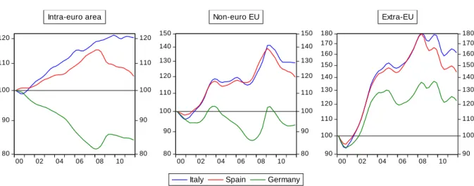
only about one quarter of GDP. There is a major difference between Italy and Spain in the drivers of the improvements of the current-account balance. Spain's export performance has been even better than Germany's, but Italian exports have remained much weaker (Figure 1). Import compression has also been a major factor, especially in Spain, where domestic demand fell more significantly than in Italy.
Table 1: Main macroeconomic indicators
A. ITALY
1998-
2007 2008 2009 2010 2011 2012 2013 GDP growth
real potential 1.3 0.3 -0.3 -0.2 0.2 -0.8 -0.4
real actual 1.5 -1.2 -5.5 1.7 0.4 -2.4 -1.3
nominal 4.0 1.3 -3.5 2.1 1.7 -0.8 0.2
Output gap 1.5 1.7 -3.6 -1.8 -1.6 -3.1 -4.0
Unemployment rate 8.7 6.7 7.8 8.4 8.4 10.7 11.8
Inflation headline 2.3 3.5 0.8 1.6 2.9 3.3 1.6
constant tax 3.5 0.8 1.6 2.6 2.5
Primary budget balance
actual 2.8 2.5 -0.8 0.1 1.2 2.5 2.4
structural 1.3 0.5 0.9 1.4 4.1 4.8
Budget balance actual -2.8 -2.7 -5.5 -4.5 -3.8 -3.0 -2.9
structural -3.8 -4.2 -3.7 -3.6 -1.4 -0.5
Gross public debt 107.2 106.1 116.4 119.3 120.8 127.0 131.4
Current account balance -0.2 -2.9 -2.0 -3.5 -3.1 -0.5 1.0
Net International Investment
Position -13.2 -24.1 -25.3 -23.9 -20.7 -24.4
B. SPAIN
1998-
2007 2008 2009 2010 2011 2012 2013 GDP growth
real potential 3.4 2.5 0.9 0.3 -0.2 -0.9 -1.4
real actual 3.8 0.9 -3.7 -0.3 0.4 -1.4 -1.5
nominal 7.7 3.3 -3.7 0.1 1.4 -1.3 0.1
Output gap 1.4 0.5 -4.2 -4.7 -4.1 -4.6 -4.6
Unemployment rate 11.1 11.3 18.0 20.1 21.7 25.0 27.0
Inflation headline 3.0 4.1 -0.2 2.0 3.1 2.4 1.5
constant tax 4.2 -0.4 1.3 2.4 1.7
Primary budget balance
actual 2.5 -2.9 -9.4 -7.7 -7.0 -7.7 -3.2
structural -2.9 -6.8 -5.5 -4.8 -2.5 -1.0
Budget balance actual -0.1 -4.5 -11.2 -9.7 -9.4 -10.6 -6.5
structural -4.5 -8.5 -7.4 -7.2 -5.5 -4.4
Gross public debt 50.8 40.2 53.9 61.5 69.3 84.2 91.3
Current account balance -5.2 -9.6 -4.8 -4.4 -3.7 -0.9 1.6
Net International Investment
Position -47.0 -79.3 -93.7 -88.8 -90.6 -91.4
Source: Net International Investment Position from Eurostat, all other indicators from AMECO, which is based on the May 2013 forecast of the European Commission. Note: percent change for GDP growth; percent of GDP for all other variables.
Figure 1: GDP and its main components (2007Q4=100, at constant prices), 2005Q1-2013Q1
Source: Eurostat. Note: data is seasonally adjusted and adjusted data by working days
The calculations and literature survey presented in Darvas (2012b) suggest that the ULC-based real effective exchange rate (REER) is strongly related to export performance. Figure 2 shows that the ULC-REER relative to euro-area partners has not yet adjusted in Italy – the euro-area country that faced the highest pre-crisis real appreciation. The REER calculated against non-euro area countries depreciated somewhat, largely because of the nominal depreciation of the euro from its highly overvalued rate in 2007, but the index is still much stronger than the historical average.
Spanish data looks better, and the fall in REER is in line with the excellent export performance.
However, ULC improvements were largely achieved through labour shedding (Darvas, 2012a) and the large external debt requires further improvements in net exports.
Figure 2: ULC-based real effective exchange rate (2000Q1=100), 2000Q1-2011Q4
Source: the updated dataset of Darvas (2012a). Note: The indicators refer to the business sector excluding agriculture, construction and real estate, calculated with constant sectoral weights. Since the indicators are noisy, we show the Hodrick-Prescott filtered values calculated with smoothing parameter 1, a very low value, to get rid of the short term noise only.
115 110 105 100 95 90 85 80 75
115 110 105 100 95 90 85 80 75 2006 2008 2010 2012
GDP Domestic demand Exports of goods and services Imports of goods and services
Italy 115
110 105 100 95 90 85 80 75
115 110 105 100 95 90 85 80 75 2006 2008 2010 2012
Spain 115
110 105 100 95 90 85 80 75
115 110 105 100 95 90 85 80 75 2006 2008 2010 2012
Germany
120
110
100
90
80
120
110
100
90
80
00 02 04 06 08 10
Intra-euro area
150 140 130 120 110 100 90
80
150 140 130 120 110 100 90
80
00 02 04 06 08 10
Italy Spain Germany Non-euro EU
180 170 160 150 140 130 120 110 100 90
180 170 160 150 140 130 120 110 100 90
00 02 04 06 08 10
Extra-EU
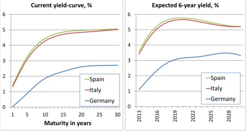
The markets’ assessments of the sustainability of public finances can be reflected in the secondary market yields of government bonds. Italian and Spanish yields still well exceed the yields in Germany (Figure 3, left panel). We calculated, using the expectation hypothesis of the term structure (EHTS), the expected yields in the three countries (Figure 3, right panel)6. We report the results for the 6-year yields, because the duration of public debt is typically about 6 years and therefore the 6-year yield is a simple and reasonable proxy for the average cost of new borrowing. According to this measure of expectations, yields are expected to increase in all three countries in the next 5-8 years, after which yields are expected to remain broadly stable. The average expected spread relative to Germany of the 6-year yield from 2014-2030 is 227 basis points for Italy and 239 basis points for Spain, using market yields of 22 August 2013.
Figure 3: Current and expected government bond yields, based on yields of 22 August 2013
Source: Bruegel calculations using data from Datastream. Note: For the yield curve, all yearly maturities up to 10 years, plus 15/20/30 years were mostly available. We interpolated other maturities and used the Hodrick-Prescott filter (=10) to smooth the yield curve. The expected yield is calculated on the basis of the smoothed yield curve, using the expectation hypothesis of the term structure (EHTS) and assuming no term premium.
3. How to foster ULC-REER adjustment?
We argue that beyond the vitally important structural reform agenda, further real exchange-rate depreciation should play a major role in fostering the external sustainability of countries with large negative net IIP, like Spain. Italy does not have a large negative IIP, but its exports have long been losing market share and its economic growth was low even before the crisis. Real exchange rate depreciation could foster the development of the tradable sector, which in turn could improve overall economic growth, because productivity growth in the tradable sector is typically faster than in other industries.
Since euro-area member countries do not have a stand-alone currency, internal devaluation should foster this adjustment. In this regard, there are two important factors:
6 For example, arbitrage should ensure that the current 2-year yield is the average of the current 1-year yield and the expected 1-year yield one year from now.
0 1 2 3 4 5 6
1 5 10 15 20 25 30
Maturity in years Current yield-curve, %
Spain Italy Germany
0 1 2 3 4 5 6
2013 2016 2019 2022 2025 2028
Expected 6-year yield, %
Spain Italy Germany
Fiscal consolidation and internal devaluation are interrelated;
Developments in other euro-area countries, including fiscal policy developments, have crucial impacts on the adjustment that southern euro-area members need to achieve.
By definition, domestic ULC declines if production increases, employment falls, and the hourly wage rate falls, all other things being equal. Certainly, the most benign way of reducing ULC is faster technological development, which results in increased productivity and thereby production, if labour input is unchanged. But stimulating such technological development is easier said than done. Without sudden improvements in technology, ULC can be reduced by cutting employment (relative to output) and/or by reducing wages. Arguably, adjusting through higher unemployment is socially less
preferable than adjusting through lower wages. When wages are rigid downward, domestic
macroeconomic policies can have a role in reducing them. Fiscal consolidation depresses output and employment, but also depresses prices and wages and therefore most likely reduces ULC too.
Therefore, fiscal consolidation can help – even if through a painful process – to restore price competitiveness. But in turn, lower prices increase the real value of the debt, thereby endangering debt sustainability.
ULC should always be looked at relative to the ULC of trading partners. The left hand panel of Figure 2 showed that while Spanish ULC relative to other euro-area countries has fallen significantly since 2008, Italian ULC did not and German ULC increased only slightly. The Spanish ULC fall was largely the consequence of massive layoffs (Darvas, 2012a). Therefore, if there is no sufficient increase in German ULC and that other ‘northern’ euro-area trading partners, countries in southern Europe will need deflation (which worsens debt sustainability) or further massive layoffs (which endangers social stability). In their elegant analytical paper, Merler and Pisani-Ferry (2012) also showed that the relative fiscal position between ‘north’ and ‘south’ matters, ie if there is more fiscal consolidation in the north, even more is needed in the south.
4. Public debt simulations
We use a simple numerical model with a few behavioural equations and a number of accounting identities to simulate debt trajectories. We highlight that our goal is not to produce a forecast: that would require more detailed data, precise estimation of behavioural parameters, and above all, long- horizon forecasts for the driving variables, such as economic growth, inflation and budget balance.
Instead, we make plausible assumptions within a simple and transparent model to assess various scenarios, and the differences between the scenarios. Box 1 summarises the main assumptions.
Box 1: Baseline assumptions for the public debt simulations
We make the following numerical and behavioural assumptions for the baseline scenario:
We take the end-2012 public debt stock and European Commission’s May 2013 forecast for budget balance and GDP growth for 2013 as the starting point.
By now, the situation with budget deficits, debts and the economic outlook is slightly worse than the May 2013 forecasts. However, there is no up-to-date comprehensive forecast for all of the required
macroeconomic indicators and our focus is on the medium- and long-run simulations, which would be only marginally affected by a more up-to-date forecast for 2013.
Potential GDP growth gradually increases by 0.1 percentage point per year from zero to 1 percent per year in 10 years.
This assumption is similar but slightly more conservative than the baseline scenario in Italy’s stability programme, which assumes that potential growth increases from about zero in 2013 to about one percent by 2018 and stays at this level thereafter. Spain’s stability programme assumes a negative potential GDP growth rate at least until 2016 (the table in the stability programme presents yearly data only up to 2016) and an average 1.2 percent per year rate in 2017-21, assumptions that do not differ much from ours.
The baseline GDP deflator change is 1 percent per year.
This assumption is more conservative than the assumption in Italy’s stability programme, which assumes an average 1.8 percent yearly change in the GDP deflator from 2013-18. Our choice is motivated by what we see as a major need for a price competitiveness adjustment. We note that the baseline inflation is altered when there is a change in the cyclical position of the economy, as described by the Phillips-curve relationship below.
Phillips-curve is rather flat: a 1 percent lower output gap reduces prices by 0.1 percent.
There have been major fiscal adjustments in Italy and Spain, yet prices have not declined, suggesting that prices are sticky and the Philips-curve has to be flat7. The Phillips-curve may change because of, for example, structural reforms that make prices and wages more responsive to the cyclical position of the economy. However, it takes time for structural reforms to have an effect and in our model the output gap gradually reverts to zero (see the next point) and the Phillips-curve matters only while the gap is non-zero.
If there are no other shocks and no change in the structural primary balance, then the output gap improves by 1 percent of GDP per year, until zero is reached.
This assumption is broadly in line with the assumption in Italy’s stability programme, which assumes that the current 4.8 percent of GDP output gap corrects by about 1 percent per year in the next four years, and the then remaining approximately one percent gap is corrected by about one-third of a percent per year in the following three years.
The potential growth rate and the closure of the output gap define the real GDP growth rate8, and the real GDP growth rate and the change in the GDP deflator determine the nominal GDP growth rate.
We define the fiscal effort as the change in the structural primary balance.
7 The increase in consumption taxes also contributed to inflation in the midst of the deep crisis, yet the constant-tax consumer price indicator of Eurostat suggests that underlying inflation was relatively high
considering the depressed state of the economy, high unemployment and the need for a relative price adjustment between euro-area countries. Also, in Ireland the GDP deflator fell, suggesting that the Irish economy is more flexible than the economies of southern Europe.
8 For example, if potential growth is 0.2 percent per year and 1 percent of GDP output gap is corrected, then real GDP growth is 1.2 percent.
There is now an extensive literature arguing that this is not the best measure, partly because the structural balance calculations are imperfect. Yet this is the most widely used indicator and it is very easy to link this indicator to public debt simulations.
The fiscal multiplier is only instantaneous (within the year) and its value is 1, which implies that a 1 percent of GDP higher structural primary surplus reduces the output gap by 1 percent.
There is an intense debate about the size of fiscal multipliers, which also depend on the composition of fiscal adjustment and the economic cycle. Some empirical papers argue that fiscal adjustment not only has an instantaneous effect, but an effect spreading across several years. Yet there is a
controversy regarding the magnitude of fiscal multipliers and uncertainty about the composition of future fiscal adjustment, which implies that it is not possible to make a sound assumption about the multiplier. Our assumption should not be that far from the ‘middle’ of the range of the typical assumptions on the multiplier, given the depressed states of the economies of Italy and Spain. Also, our assumption is simple, thereby helping to keep our calculations transparent.
Structural primary surplus as % of GDP:
o Italy: tiny change from a 4.8 percent surplus in 2013 to 5.0 percent from 2014 onwards;
o Spain: 1 percent per year improvement from -1 percent in 2013 to 5 percent in 2019;
o In both countries, the 5 percent primary surplus is maintained in the long run.
This assumption is less ambitious than the assumption in Italy’s stability programme, which assumes a 6.1 percent cyclically adjusted primary surplus from 2016 onwards. However, we see the difficulties in implementing further fiscal consolidation measures when unemployment is high. Also, over the last 50 years, no OECD country (except Norway, thanks to oil surpluses) has sustained a primary surplus above 5 percent of GDP. Even sustaining a 5 percent of GDP primary surplus (our assumption) for several decades may prove to be politically challenging.
The gap between the structural and actual primary balance is 0.5 times the output gap.
For example, when the structural primary surplus is 1 percent of GDP and the output gap is minus 4 percent of GDP, then the actual primary deficit is 1 percent of GDP. We make assumptions about the structural primary balance as a measure of fiscal effort (see above), but for calculating the debt stock, the actual (primary and overall) balance is needed.
No additional privatisation revenues.
While both countries plan to privatise, we remain on the conservative side by not assuming any privatisation revenue.
Expected future interest rates (ie the cost of borrowing in future years) are as implied by the expectation hypothesis of the term structure, with the assumption of no term premium.
We note that the expected yield can be the average of two major outcomes, such as a benign scenario (in which the southern countries will gain control over their public debt and the spread to Germany falls) and a catastrophic scenario (in which the southern countries do not gain control over their public debt and an unpredictable scenario would emerge). Politicians may argue that markets wrongly over-
estimate the probability of the catastrophic scenario, and therefore in the benign scenario spreads to Germany will be lower than the current expectation. However, since government bonds with various maturities are traded on the market, the expectation hypothesis of the term structure (EHTS) should provide the best guide to expected future interest rates. Assuming lower interest rates compared to market expectations would amount to wishful thinking.
A drawback of the use of market-implied expected interest rates is that they are consistent with current market expectations of various variables, such as inflation, growth and budget balance, expectations that are not known for the 20-year period of our simulations. This implies that the assumption we make for all the variables may not be consistent. However, this drawback applies to all public debt simulations, including those of the IMF and European Commission.
We use the expected 6-year maturity yields as a proxy of the cost of new borrowing.
Since the duration of public debt is about 6 years, using the 6-year yields is a simple and straightforward choice.
Finally, we highlight an assumption that we do not make: the interrelationship between potential growth and the adjustment of the real exchange rate.
We cannot exclude that a faster downward adjustment in the real exchange rate would facilitate the development of the tradable sector. But because productivity growth used to be faster in the tradable than in the non-tradable sector, a faster reallocation of resources toward to tradable sector could increase aggregate productivity growth, and thereby potential growth of the whole economy. While we believe that such an interrelationship exists, its quantification would rely on arbitrary assumptions that we wished to avoid.
END OF BOX
We calculate four scenarios for the public debt ratio:
Baseline, as described in Box 1.‘Low German wages’: What if German inflation remains low and therefore Italy and Spain need to reach zero inflation to achieve the required competitiveness adjustment? In this scenario, inflation in Germany is 2 percent, zero in Italy and Spain and the euro- area average is 1 percent, instead of our baseline assumption of 3 percent inflation in Germany, 1 percent in Italy and Spain, and 2 percent in the euro area. ‘Fiscal fatigue’: What if the fiscal commitments are weakened and the 5 percent of GDP primary surplus is not sustained? In this scenario, after three consecutive years with 5 percent of GDP structural primary surplus, the primary surplus is reduced to 4 percent of GDP. We note that this is a rather small reduction in the primary surplus in light of the historical volatility of this variable.‘OMT activated’: What if the interest rate spread to Germany is reduced from the current 227-239 basis points to 150 basis points? Such a reduction could be the consequence of the activation of the ECB’s Outright Monetary Transactions (OMT), which in turn necessitates applications by Italy and Spain for either a full or a precautionary macroeconomic adjustment programme from the European Stability Mechanism (ESM). Of these scenarios, the last requires further qualification. In the summer of 2012, Italian and Spanish yields started to increase very rapidly, despite various ECB measures, such as the two rounds of 3-year long
term refinancing operations (which provided unlimited and cheap liquidity to banks)9, and efforts by European heads of state, such as the June 2012 declaration on the design of a European banking union to sever the link between banks and sovereigns. But there was no lender of last resort for euro-area sovereigns at that time.
As highlighted by De Grauwe (2011), multiple equilibria can characterise a monetary union in which there is no lender of last resort for sovereigns of individual states. In the ‘bad equilibrium’, financial markets can force these countries’ sovereigns into default and perhaps even an exit from the monetary union, but they could not if there was a lender of last resort. The lack of such a backstop is not a substantial problem when the level of debt is low10, but the debts of Italy and Spain were either high or rapidly rising.
In the heightened situation during the summer of 2012, ECB announcements acted like a magic wand:
Italian and Spanish bond yields fell sharply without any actual intervention. The first announcement was the remarkable “whatever it takes” speech of ECB President Draghi on 26 July 2012 (Draghi, 2012), pledging to use every means available to a central banker to stabilise the euro, at least within the mandate of the ECB. This was followed on 6 September 2012 by the decision of the ECB Governing Council to establish a new government-bond purchasing programme, called Outright Monetary Transactions (OMT). OMT will be unlimited in principle, will treat the ECB pari passu with other creditors, and will be based “strict and effective conditionality attached to an appropriate European Financial Stability Facility/European Stability Mechanism (EFSF/ESM) programme”
(ECB, 2012). The financial assistance programme can be full or precautionary. Currently, no country qualifies for the OMT.
Has the OMT announcement in September 2012 led to the ‘good equilibrium’, ie a situation in which government bond yields of euro-area members are solely determined by their fundamental economic and fiscal conditions, and not fears of an eventual euro exit? The answer is no, for the simple reason that there is still uncertainty about the actual deployment of the OMT. In order to be eligible for the OMT, Italy and Spain need to apply for a financial assistance programme. Such an application can only result from a complicated negotiation process involving all euro-area governments, the ECB, the European Commission and possibly the IMF. It is not clear what the result of such negotiations would be. Financial assistance programmes for Italy and Spain, even if precautionary, would necessitate a significant increase in the resources of the ESM. Active OMT programmes for Italy and Spain might involve the purchase by the ECB of a significant amount of Italian and Spanish government debt, which would increase the risks for the ECB. Those euro-area members in which decision makers believe that they have reached the limits of the solidarity they can provide to other euro-area countries, may be reluctant to agree to such a programme, or the programme may not be
comprehensive enough. Even if a country is eligible for the OMT, the ECB has the right to decide when and how much to purchase (if at all). The interest rate at which the ECB would intervene in government bond markets is also uncertain. There are therefore so many uncertainties that the actual approval of a financial assistance programme for Italy and Spain, the increase in the ESM's resources, and an actual purchase of government bonds by the ECB must reduce the spread of Italy and Spain relative to Germany, which was expected to be around 227-239 basis points on average during 2014- 2030 on 22 August 2013 at the 6-maturity (as we use in our simulations).
9 See Darvas and Savelin (2012) for the developments of the Italian, Spanish and German government bond yields after ten auctions of the ECB between January 2010 and October 2012.
10 For example, in the US, the Federal Reserve does not buy the debt of states such as California or New York (which have debt of about 10 percent of GDP), but buys only federal bonds.
We stress that our assumption for the reduction of the spread from current 227-239 basis points to 150 basis points is purely hypothetical. No one can guess how much yields would decline as a
consequence of an ECB government bond purchase under the OMT.
We also note that if Italy and Spain were under a financial assistance programme (which is a
necessary condition of OMT), they could also borrow from the ESM (and possibly from the IMF) at a lower borrowing rate than the 150 basis points spread over the German bunds as assumed in our Scenario 411. But since our purpose with this scenario is only illustrative, we did not add a fifth scenario in which Italy and Spain borrow from the ESM.
Let us now turn to the results of the simulations and start with the baseline scenario. In Figure 4, we compare our baseline scenario to the IMF’s April 2013 projection and the debt trajectory implied by the new debt rule. The IMF projection goes to 2018. For both countries, our baseline scenario is slightly more optimistic than the IMF’s projection during this period. Our longer-term projection suggests that the debt ratio will continue to fall in Italy and will start to fall in Spain after 2020 from a level of about 110 percent of GDP, but the pace of debt ratio reduction is relatively slow12.
The so-called ‘Six-Pack’, adopted by all EU member states in 2011, operationalised the public debt ratio rule of the Stability and Growth Pact (SGP): the gap between the actual debt level and the 60 percent of GDP reference should be reduced by 1/20th annually (on average over 3 years)13. As a transitional arrangement, each member state in excessive deficit procedure is granted a three-year period following the correction of the excessive deficit for meeting the debt rule. Italy’s excessive deficit procedure was abrogated in the summer of 2013 and therefore we calculated the debt ratio trajectory implied by the debt rule after 2016. Spain’s new deadline to exit the excessive deficit procedure is 2016 and therefore we calculated the debt rule trajectory after 2019.
Figure 4 shows that debt ratio reduction under our baseline scenario does not meet the requirements of the operationalised debt rule of the SGP. The gap between the baseline scenario and the debt rule trajectory is especially wide, and widening, in the case of Italy. For Spain, the main issue is that the debt ratio reduction starts later than the required date, though when the debt ratio reduction is projected to start, its pace is broadly in line with the fiscal rule.
11 The ESM lends at its own borrowing costs plus a minuscule surcharge. The ESM has not yet issued bonds. The spread of the EFSF bond over German bunds was about 55 basis points on 22 August 2013 at the 6- year maturity. The ESM may borrow from markets at a slightly lower rate than the EFSF.
12 One reason for small debt reduction after 2017 in Italy and after 2023 in Spain is that GDP growth is no longer boosted by the closure of the output gap. As implied by the assumptions made in Box 1, the output gap is eliminated in the next four years in Italy, and from 2019 to 2023 in Spain (until then, the yearly fiscal consolidation exactly offsets the autonomous correction of the output gap).
13 See http://europa.eu/rapid/press-release_MEMO-11-898_en.htm .
Figure 4: Public debt/GDP ratio: our baseline scenario, IMF’s April 2013 projection and the trajectory implied by the new debt ratio rule
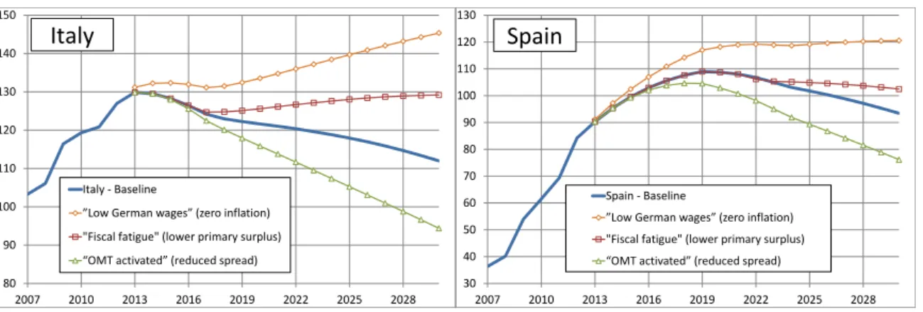
Figure 5 shows the results of the three alternative scenarios, ‘Low German wages’, ‘Fiscal fatigue’
and ‘OMT activated’. The figure demonstrates that debt trajectories are very sensitive to alterations in the assumptions. If inflation has to be zero, instead of 1 percent as assumed in the baseline, the debt ratio explodes in Italy and stabilises at about 120 percent of GDP in Spain. If fiscal commitments are weakened and the primary surplus is reduced from 5 to 4 percent of GDP (which is a rather small reduction), the debt ratio increases rather than falls in Italy, and the pace of Spanish debt reduction abates. By contrast, if the spread is reduced from 227/239 to 150 basis points relative to Germany, the reduction in the debt ratio is much faster.
Figure 5: Public debt/GDP ratio: alternative scenarios
5. Trade-offs
Using the model described in the previous section, we can quantify various trade-offs. First, we assess the situation in which inflation has to be 1 percent lower because of low German inflation, in order to support the necessary competitiveness adjustment between southern euro-area members and Germany. If inflation is 1 percentage-point per year lower, to have
0 10 20 30 40 50 60 70 80 90 100 110 120 130
2007 2010 2013 2016 2019 2022 2025 2028
Italy - Baseline
Italy - IMF April 2013 projection Italy - New EU debt rule Spain - Baseline
Spain - IMF April 2013 projection Spain - New EU debt rule
80 90 100 110 120 130 140 150
2007 2010 2013 2016 2019 2022 2025 2028
Italy - Baseline
”Low German wages” (zero inflation)
"Fiscal fatigue" (lower primary surplus)
“OMT activated” (reduced spread)
Italy
30 40 50 60 70 80 90 100 110 120 130
2007 2010 2013 2016 2019 2022 2025 2028
Spain - Baseline
”Low German wages” (zero inflation)
"Fiscal fatigue" (lower primary surplus)
“OMT activated” (reduced spread)
Spain
debt dynamics similar to those in our baseline scenario, then:Either the persistent primary surplus has to be higher in Italy by 1.3 percent of GDP and in Spain by 1.0 percent of GDP,
Or the interest spread to Germany should be reduced to approximately 130 basis points in Italy and 160 basis points in Spain.
Second, we check the implications of a reduction of the spread to Germany from 227/239 to 150 basis points. In this case, in both Italy and Spain, an approximately 0.8 percent of GDP lower structural primary surplus would produce the same debt dynamics as our baseline scenario. Therefore, spread reduction would bring a major relief for fiscal consolidation.
And thirdly, we check what policy measures would help Italy and Spain to meet the operationalised fiscal rule on public debt ratio reduction. As we have argued, for Spain the issue is that debt reduction starts later. Therefore, for Spain the deadline for exiting the excessive deficit procedure has to be extended by about two or three more years beyond the current deadline of 2016. If we replace our baseline assumption with:
Either a 0.9 percent of GDP higher primary surplus in Italy and 0.2 percent in Spain,
Or 0.7 percentage point per year higher inflation in Italy and 0.3 percentage point in Spain, Or about 90 basis points lower interest rate spread to Germany in Italy and about 10 basis points lower spread in Spain,
then the debt ratio by 2030 would be the one implied by the operationalised debt rule as depicted in Figure 4. Therefore, meeting the operationalised SGP debt rule would not require a major effort from Spain, but Italy would need to make more effort. The difference between the two countries is
explained by the difference in debt levels: since Italy has a significantly higher debt level, but in our baseline assumption we assume the same growth, inflation and primary balance for the two countries, Italy needs to do more to reduce her debt.
6. Conclusions
The Italian and Spanish economies are depressed with large negative output gaps and high
unemployment. Italy has a large structural primary surplus (4.8 percent in 2013 according to the May 2013 forecast of the Commission), but Spain is still expected to have a structural primary deficit of 1 percent, necessitating a major fiscal adjustment in the years ahead. Unit labour costs have not yet adjusted in Italy and have adjusted through labour shedding in Spain; further adjustment is needed in both countries. There is some, but insufficient, market confidence, which is reflected in the 227 (Italy) and 239 (Spain) basis points expected 6-year maturity spread relative to German bunds from 2014- 2030. According to our baseline scenario for public debt, the projected pace of debt ratio reduction is too slow in Italy, missing the requirements of the SGP operationalised debt rule by a wide margin. In Spain the debt ratio is even expected to increase until about 2020 before starting to decline gradually afterwards, ie about 2/3 years after the operationalised debt rule applies to Spain, should the country exit the excessive deficit procedure by the current deadline of 2016. And there are major risks because of the high public debt ratios: even small negative deviations from our assumptions, such as a
somewhat lower long-term growth, inflation and primary surplus, could easily result in a runaway debt trajectory.
These simulation results paint a bleak picture. Perhaps we were too conservative in making our baseline assumptions. Economic growth might pick-up faster and to a higher level than what we assumed. The tradable sector might improve without further real exchange rate depreciation. Future interest rates might be lower compared to current market expectations. But merely hoping for such benign outcomes would amount to wishful thinking. Instead, forceful policies are needed to pursue the dual goal of debt sustainability and improved price competitiveness, beyond the badly needed structural reforms aimed at fostering labour and product market flexibility, greater public sector efficiency, and banking sector clean-up.Further fiscal consolidation beyond the 5 percent primary surplus we assumed might be an option. However, the case for further fiscal consolidation is weak in the short and medium terms, when both Italy and Spain have depressed economic conditions, and high and rising unemployment. For the longer term, history teaches us a lesson in caution. Over the last 50 years, no OECD country (except Norway, thanks to oil surpluses) has sustained a primary surplus above 5 percent of GDP. Even sustaining a 5 percent of GDP primary surplus (our assumption) for several decades could prove to be politically challenging. Moreover, further fiscal consolidation may not do much to help the competitiveness adjustment when the Phillips-curve is quite flat (implying that an even greater negative output gap and even higher unemployment might not do much to reduce prices and wages). Even if the Phillips-curve becomes steeper (ie prices and wages respond more to changes in unemployment) due to structural reforms that enhance the flexibility of labour and product markets, when there is a 5 percent of GDP structural primary surplus, as we assumed in our baseline scenario, there is a very little room for further fiscal consolidation to depress output, employment, and thereby prices and wages.
Instead of faster and larger fiscal consolidation in Italy and Spain relative to our baseline assumption, we see four complementary options to help Italy and Spain (and other southern euro-area members) to achieve the dual goal of fiscal sustainability and improved price competitiveness, beyond the
necessary domestic structural reforms.
First, a more symmetric intra-euro area price adjustment should facilitate intra-euro area
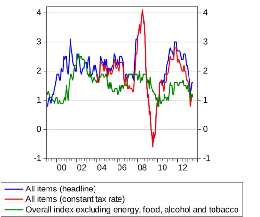
competitiveness adjustment. If inflation has to be 1 percentage point lower in Italy and Spain because the overall euro-area inflation rate undershoots the two percent target, the persistent primary surplus has to be higher in Italy by 1.3 percent of GDP and in Spain by 1.0 percent of GDP, according to our calculations. Consistent with the ECB mandate, average inflation in the euro area should not be allowed to fall below the two percent target, and Germany and other euro-area countries with a strong competitive position should refrain from domestic policies that would prevent domestic inflation from rising above two percent (Wolff, 2012; Darvas, Pisani-Ferry and Wolff, 2013). Therefore, the ECB should do whatever it takes, within its mandate, to ensure that inflation does not fall below the 2 percent target. In July 2013, the headline inflation rate in the euro area was below target at 1.6 percent (compared to the same month of the previous year). But as Vihriälä (2013) argues, the underlying inflation trends are better reflected in indicators excluding volatile food and energy prices and the impact of tax hikes induced by fiscal consolidation programmes. As Figure 6 shows, the inflation rate excluding energy, food, alcohol and tobacco was 1.1 percent in July 2013 and the constant tax rate inflation rate was 1.2 percent, suggesting that we are heading toward the ‘Low German inflation’
scenario of our simulations14.
14 The constant-tax inflation indicator is not available for the aggregate excluding energy, food, alcohol and tobacco. Since the constant-tax all items inflation is below the headline inflation, the constant tax inflation of the aggregate excluding energy, food, alcohol and tobacco is now likely below 1 percent per year, suggesting that the underlying inflationary trend largely undershoots the 2 percent target.
Figure 6: Euro-area inflation (compared to the same month of the previous year), 1999-2013
Source: Eurostat
Second, keeping inflation on target, which would require further monetary easing, would weaken the euro, which in itself would greatly facilitate adjustment in southern euro-area members. This is because the role of intra-euro trade has gradually declined, while the role of extra-euro trade has increased. A weaker euro would also boost exports, growth, inflation and wage increases in Germany, thereby helping further intra-euro adjustment, while the impact on Italian and Spanish wages would be limited because of high unemployment (Darvas, 2012b). The ECB has a neutral stance on the euro’s exchange rate and this position will not change. But the difficulties of intra-euro
competitiveness adjustment, the risks of an eventually less successful adjustment, and more generally, the downside risk to the euro-area’s economic outlook, should make the ECB more open to further measures leading to an even more accommodative monetary policy stance, when inflationary
expectations are below 2 percent. The ECB has to do only what other major central banks have done, and not more. This would weaken the euro’s exchange rate15.
Third, the growth problem should be better addressed both in southern Europe and in other euro-area countries, beyond the vitally-needed structural reforms. Economic growth is the key parameter in debt
15 We note that a weaker euro exchange rate may increase the euro-area current account surplus. The euro area’s current account is expected to reach a surplus of about 2 percent of GDP in 2013, after a decade of being almost balanced. The two main surplus countries, Germany and the Netherlands, have slightly larger surpluses, while formerly deficit countries are now moving toward a balanced position. The increased euro-area current account surplus was largely absorbed by smaller surpluses in emerging countries, which was the right way of adjustment (Darvas, 2012b). In the future, euro-area countries with large surpluses should boost their domestic demand, which would reduce their surpluses, and thereby the external surplus of the euro area would not widen too much.
-1 0 1 2 3 4
-1 0 1 2 3 4
00 02 04 06 08 10 12
All items (headline)
All items (constant tax rate)
Overall index excluding energy, food, alcohol and tobacco
sustainability. To help break out of the downward economic spiral that southern euro-area member states face, a very significant European investment programme is needed for southern members. The European Investment Bank seems to be the best institution to carry out such an investment
programme. But much more capital should be provided to it beyond the €10 billion agreed as part of 2012’s ‘Compact for Growth and Jobs’, and the internal procedures of the EIB should be revived to allow for much faster disbursement of investment. Furthermore, weak growth in the rest of the euro area has a negative impact on southern European countries too. Fostering growth throughout the euro area should be a top priority. Beyond the vitally important structural reform agenda, the euro-area’s banking problems need to be assessed properly and bank resolution and recapitalisation should be urgently pursued (Darvas, Pisani-Ferry and Wolff, 2013). This should be followed by a more appropriate fiscal policy stance in those euro-area countries that have fiscal space (Darvas, 2013).
Finally, if all else fails, the ECB will have to use its OMT to reduce interest rate spreads. Our simulation indicates that Italy and Spain would greatly benefit from a reduced interest rate on new borrowing. Reduction of the interest rate spread to Germany from the currently expected 227/239 basis points to 150 basis point would allow a 1.1 percent of GDP lower primary budget surplus, according to our calculations. Introduction of Eurobonds, ie joint borrowing by euro-area member states, is not a realistic option in the foreseeable future. Therefore, as we have discussed in detail, the best option to achieve a lower interest rate is the activation of the ECB’s OMT programme, which in turn would necessitate Italian and Spanish applications for at least a precautionary financial assistance programme, and an increase in the resources of the ESM16. In terms of adjustment requirements, this would not lead to much change, because the two countries are anyway obligated to follow the European Council's recommendations because they are under the Macroeconomic Imbalances Procedure. Also, Spain already has a banking programme from the EFSF with conditionality for the banking sector. It is quite unlikely that a precautionary programme would make many other demands compared to what the two countries have to do anyway. Yet it may prove to be difficult to agree on financial assistance programmes for Italy and Spain and to increase the resources of the ESM, and the euro area may not easily survive a scenario in which the ECB has to buy large amounts of Italian and Spanish public debt.
References
Darvas, Zsolt (2012a) ‘Compositional effects on productivity, labour cost and export adjustments’, June, Policy Contribution 2012/11, Bruegel, http://www.bruegel.org/publications/publication- detail/publication/730-compositional-effects-on-productivity-labour-cost-and-export-adjustments/
Darvas, Zsolt (2012b) ‘Intra-euro rebalancing is inevitable, but insufficient’, August, Policy Contribution 2012/15, Bruegel, http://www.bruegel.org/publications/publication-
detail/publication/747-intra-euro-rebalancing-is-inevitable-but-insufficient/
Darvas, Zsolt and Li Savelin (2012) ‘Chart of the week: the ECB’s power on Spanish and Italian bond yields’, 10 October 2012, Bruegel blog, http://www.bruegel.org/nc/blog/detail/article/913-chart-of- the-week-the-ecbs-power-on-spanish-and-italian-bond-yields/
16 Spain’s current financial sector programme does not qualify the country for an OMT programme. For an OMT, either a full EFSF/ESM macroeconomic adjustment programme or a precautionary programme has to be in place. See: http://www.ecb.int/press/pr/date/2012/html/pr120906_1.en.html.
Darvas, Zsolt (2013) ‘A new direction for euro-area macro policies’, 1st of March, Bruegel blog, http://www.bruegel.org/nc/blog/detail/article/1032-a-new-direction-for-euro-area-macro-policies/
Darvas, Zsolt, Jean Pisani-Ferry and Guntram B. Wolff (2013) ‘Europe's growth problem (and what to do about it)’, April, Policy Brief 2013/03, Bruegel,
http://www.bruegel.org/publications/publication-detail/publication/776-europes-growth-problem-and- what-to-do-about-it/
Draghi, Mario (2012), Speech by Mario Draghi, President of the European Central Bank at the Global Investment Conference in London 26 July 2012,
http://www.ecb.int/press/key/date/2012/html/sp120726.en.html
European Central Bank (2012) ‘Technical features of Outright Monetary Transactions’, Press Release, 6 September 2012, http://www.ecb.europa.eu/press/pr/date/2012/html/pr120906_1.en.html
Reinhart, Carmen M. and Kenneth Rogoff (2011) ‘A Decade of Debt’, Working Paper No. w16827, NBER
Merler, Silvia and Jean Pisani-Ferry (2012) ‘The simple macroeconomics of North and South in EMU’, Working Paper 2012/12, Bruegel, http://www.bruegel.org/publications/publication- detail/publication/740-the-simple-macroeconomics-of-north-and-south-in-emu/
Vihriälä, Erkki (2013) ‘Euro area adjustment in a low inflation environment’, 20 August 2013, Bruegel blog, http://www.bruegel.org/nc/blog/detail/article/1140-euro-area-adjustment-in-a-low- inflation-environment/
Wolff, Guntram B. (2012) ‘Arithmetic is absolute: euro area adjustment’, Policy Contribution 2012/09, Bruegel, http://www.bruegel.org/publications/publication-detail/publication/724-arithmetic- is-absolute-euro-area-adjustment/