Trajectory convergence from coordinate-wise decrease of quadratic energy functions, and applications to platoons

Trajectory convergence from coordinate-wise decrease of quadratic energy functions, and applications to platoons

Julien M. Hendrickx, Balazs Gerencs´er and Baris Fidan

Abstract— We consider trajectories where the sign of the derivative of each entry is opposite to that of the corresponding entry in the gradient of an energy function. We show that this condition guarantees convergence when the energy function is quadratic and positive definite and partly extend that result to some classes of positive semi-definite quadratic functions including those defined using a graph Laplacian. We show how this condition allows establishing the convergence of a platoon application in which it naturally appears, due to deadzones in the control laws designed to avoid instabilities caused by inconsistent measurements of the same distance by different agents.

I. INTRODUCTION

We consider trajectoriesx(t) :R+→Rⁿ that satisfy the following coordinate-wise condition

˙

xi·(∇V(x))i ≤0, ∀i= 1, . . . , n (1) for some quadratic energy function V. Intuitively, this just requires that when a coordinate of x changes, this change happens in a way that does not increase the energy function, but there is no requirement about the magnitude of the decrease, if any. We show that condition (1) guarantees convergence of x to a constant vector when the function V is positive definite, and partly extend this result to classes of positive semi-definite functions. We prove in particular that convergence is still guaranteed when the matrix defining V is a graph Laplacian, so that V is a measure of the

“disagreement” between the xi.

Condition (1) appears naturally in certain multi-agent dy- namics, including in the platooning problem we will analyze in Section III, which involves control laws with deadzones to remove potential instabilities resulting from incoherent measurements of the same distance by different agents. And indeed, we came across condition (1) when trying to establish the convergence of the system of Section III.

J. Hendrickx is with the ICTEAM institute, UCLouvain (Belgium) and with the CISE, Boston University (USA). julien.hendrickx

@uclouvain.beHis work is supported by “Communaut´e franc¸aise de Belgique - Actions de Recherche Concert´ees” and a WBI.World excellence fellowship.

B. Gerencs´er is with MTA Alfr´ed R´enyi Institute of Mathematics, Budapest, Hungary and E¨otv¨os Lor´and University, Department of Probability and Statistics, Budapest, Hungary.

gerencser.balazs@renyi.mta.hu He was supported by NKFIH (National Research, Development and Innovation Office) Grants PD 121107 and KH 126505.

B. Fidan is with the Mechanical and Mechatronics Engineering Depart- ment, University of Waterloo, ON, Canada.fidan@uwaterloo.caHis work is supported by Natural Sciences and Engineering Research Council (NSERC) of Canada under Discovery Grant 116806.

Classical approaches for establishing convergence based on energy functions rely on variation of the Lyapunov - Kraskowski - LaSalle theorems [13], [15]. These approaches apply to dynamical systems of the formx˙ =f(x, t), where the vector field f often satisfies some (uniform) continuity condition [4], [8]. For example, LaSalle theorem guarantees (under certain conditions) the convergence of solutions of

˙

x = f(x) to an invariant set, but not necessarily to a point, provided that V(x(t)) is nonincreasing everywhere [16]. Convergence to a single point is only guaranteed under additional conditions, such as _dt^dV(x(t)) being sufficiently negative, by one of the original Lyapunov theorems. Another result for time-varying systems guarantees convergence to 0 if _dt^dV(x(t))≤0 and is not identically 0 on any trajectory other than that staying at 0 [19]. Crucially, in all these results, the relevant conditions on the decrease of V and on the smoothness of V and f must be satisfied globally, and not just for the trajectory considered, otherwise the results do not hold.

Particularly in cyber-physical systems or systems involv- ing discrete computations or events, there may not be a natural way of defining a global evolution of the form

˙

x = f(x, t), for instance when external noise or control is present. Thereforexmay not contain all the information required to determine x˙ and would thus not qualify as

“the state of the system” in a classical sense. The speed

˙

x may indeed depend on various elements related to the history ofx, communications with other systems, random or arbitrary events, etc. Certain works on consensus overcome this difficulty by defining a trajectory-dependent equivalent vector field f˜x(x, t) to hide the complexity of the process, i.e. a vector field for which x˙ = ˜f_x(x, t) holds for that specific trajectory x only [9], [12], [14]. But it can be challenging to define equivalent fields satisfying the global conditions required to apply the classical convergence results, (continuity, decrease of V, suitable invariant sets...), and we indeed did not succeed in applying this approach to general trajectories satisfying (1). Moreover, we would argue that this is a cumbersome and unnatural step. Extensions of Lyapunov results to differential inclusions could also not be directly applied to (1) as they require pre-defining the invariant sets to whichxwould converge [1], [7]. Hence we think it is in many cases relevant to analyze the convergence of trajectories based purely on their properties, and not on those of a vector field or differential inclusion they follow.

Standard trajectory-focused techniques do not allow estab- lishing convergence solely based on (1). Observe it implies

arXiv:1903.00290v1 [math.DS] 1 Mar 2019

that

d

dtV(x(t)) =

n

X

i=1

(∇V(x))ix˙i≤0,

so thatV(x(t))is non-increasing and hence converging, but it is well known that _dt^dV(x(t)) ≤ 0 does not imply the convergence of x in general. There is here no guarantee on the decrease rate of V, even relative to the magnitude of x, as the gradient˙ ∇V(x) and x˙ can be orthogonal or arbitrarily close to being orthogonal. Hence the total decrease ofV cannot be directly bounded relative to the length of the trajectory, which would have guaranteed a finite length of the trajectory. We can thus a priori not exclude thatxwould keep varying while approaching a level set{x:V(x) =c}.

Moreover, these level sets are not compact whenA is only positive semi-definite.

In the following section we establish our new convergence result based on condition 1. Afterwards, we demonstrate its application for a platoon formation problem.

II. CONVERGENCE RESULT

For the simplicity of exposition, we state our main conver- gence result for quadratic functions of the form x^TAx and particularize condition (1) to these functions, but extension to general quadratic functions is immediate by a applying a constant offsetx⁰ =x−a for some vectora.

Theorem 1: LetA∈R^n×nbe a symmetric positive semi- definite matrix, and x(t) : R+ → Rⁿ be an arbitrary absolutely continuous function, also implying thatx(t)˙ exists almost everywhere. Suppose that the following two condi- tions (particularizing (1) toV(x) =¹₂x^TAx) holds for every i= 1, . . . , n:

˙

xi(t)Ai,:x(t)≤0. (2) Then

(a) If A is positive definite, x(t) converges to a constant vectorx^∗.

(b) IfA is positive semi-definite and no nonzero vector of its kernel has a zero component (w∈kerA, w6= 0⇒ wi 6= 0,∀i), then either x(t) converges to a constant vectorx^∗or every accumulation pointx¯ ofx(t)lies in kerA.

We note that condition (b) can only be satisfied if kerA has dimension 1. Indeed, ifv 6=ware linearly independent vectors in kerA, one can always find a nontrivial linear combinationz=αv+βwfor whichzi= 0for any giveni.

Proof: We first show that (b) implies (a): Indeed, with V(x) := ¹₂x^TAx, it follows from (2) thatV˙(x(t))≤0 so that x(t) always remains in the set {x : x^TAx ≤ V(0)}.

WhenAis positive definite, this set is compact andx(t)has thus at least one accumulation point. Supposing that x(t) would not converge, (b) implies that every accumulation point of x(t) would be in the kernel of A, i.e. would be equal to 0, which implies that x(t) would converge to 0 since it would be the only accumulation point. In Rⁿ, convergence of a continuous trajectory is indeed equivalent to the existence of one single accumulation point. We

therefore only need to prove (b) in the sequel.

Consider the hyperplane

K_i={x∈Rⁿ | A_i,:x= 0} (3) orthogonal to the ith row of A. If there is no accumu- lation point, or exactly one accumulation point, meaning that x(t) converges to a constant vector, the statement (b) holds trivially. We suppose to the contrary that there exist more than one accumulation point. We select an arbitrary accumulation point x¯ contained in the smallest possible number of hyperplanesKi and denote this smallest possible number byk. We will show thatx¯∈kerA. Without loss of generality, we can assume the indices are ordered in such a way that

¯

x∈K1∩K2∩. . .∩Kk,

¯

x /∈Kk+1∪Kk+2∪. . .∪Kn.

We can chooseε >0such that two following two conditions hold: (i) B(¯x,4ε)∩(Kk+1∪Kk+2∪. . .∪Kn) = ∅ and (ii) there is at least one other accumulation point outside of B(¯x,4ε) (otherwise x¯ would be the only accumulation point).

Due to the existence of this other accumulation point,x(t) must infinitely often leave B(¯x,3ε) while getting infinitely often into B(¯x, ε). More precisely, there exists a diverg- ing sequence of disjoint time intervals [t^m₁ , t^m₂] such that x(t^m₁) ∈ S(¯x, ε) = ∂B(¯x, ε), x([t^m₁, t^m₂]) ⊂ cl B(¯x,3ε) andx(t^m₂)∈S(¯x,3ε) =∂B(¯x,3ε)for every m. We define

∆x^m=x(t^m₂)−x(t^m₁ ), so2ε≤ ||∆x^m|| ≤4ε. Our proof relies on the following two lemmas, which will establish that (∆x^m)^TA∆x^m=P

i(∆x^m)_i(A∆x^m)_i→0.

Lemma 2: lim_m→∞(A∆x^m)i = 0 for i ≤ k. As a consequence,lim_m→∞∆x^m_i (A∆x^m)i= 0 fori≤k.

Proof: We first show that the distance betweenx(t^m₂) and Ki converges to 0 for every i = 1, . . . , k. If it was not the case, there would be an infinite subsequencex(t^m₂⁰) at a distance larger than δ > 0 from Ki. Since the x(t^m₂) are by definition in the compact setB(¯x,3ε), this sequence would admit an accumulation point that would have positive distance at leastδ >0fromKi. Moreover, this accumulation point could not belong to anyK_j withj > k because these sets have no intersection with B(¯x,4ε). Hence we would have an accumulation point that belongs to less thank sets K_i, which contradicts the selection of x¯as an accumulation point of x(t) belonging to the smallest possible number of Ki.

As a consequence the distance between x(t^m₂)and every Ki, converges to 0, and a similar argument shows the same result for x(t^m₁). This implies by definition of Ki that lim_m→∞(A∆x^m)i = lim_m→∞Ai:x(t^m₂)−Ai,:x(t^m₁) = 0 of i≤k. The final implication of the Lemma follows from the boundedness of∆x^m.

Lemma 3: limm→∞(∆x^m)i = 0 for i > k. As a conse- quence,limm→∞∆x^m_i (A∆x^m)i= 0 fori > k.

Proof: Fori > k, we knowB(¯x,3ε)is bounded away fromK_iby at leastε. Hence, ify∈B(¯x,3ε), then|Ai,:y| ≥

c for some c >0. So sincex_i(t^m₂), x_i(t^m₁ )∈B(¯x,3ε), we have

|xi(t^m₂)−x_i(t^m₁)| ≤ Z t^m₂

t^m₁

|x˙_i(t)|dt

≤ 1 c

Z t^m₂ t^m₁

|x˙i(t)||Ai,:x(t)|dt.

Condition (2) implies that x˙i(t)andAi,:x(t)have opposite signs whenever they are both nonzero (and also for all other indices j), hence we obtain from the previous inequality:

|xi(t^m₂ )−xi(t^m₁ )| ≤ −1 c

Z t^m₂ t^m₁

˙

xi(t)Ai,:x(t)dt

≤ −1 c

Z t^m₂ t^m₁

n

X

j=1

( ˙xj(t)Aj,:x(t))dt

=1

c(V(x(t^m₁))−V(x(t^m₂))), where we remind thatV(x) = ¹₂x^TAx. This last inequality holds for everym, so that

X

m

|x_i(t^m₂)−x_i(t^m₁)| ≤ 1 c

X

m

(V(x(t^m₁))−V(x(t^m₂ )))<∞, as V(x(t)) is non-increasing and the overall decrease of V(x(t))is finite. Therefore, there holds|∆x^m_i |=|xi(t^m₂)− xi(t^m₁)| →0asm→ ∞which we wanted to show. The last implication of the Lemma follows from the boundedness of

∆x^m.

It follows from Lemmas 2 and 3 that

m→∞lim (∆x^m)^TA∆x^m= 0. (4) We will now show that this implies that k = n, i.e. that

¯

x∈Ki for everyi, and thus thatx¯∈kerAby the definition (3) of theKi. Suppose by contradiction thatk < n, which implies that∆x^m_n →0 by Lemma 3. We claim that

lim inf

m→∞ dist(∆x^m,kerA)≥c >0, (5) for some positive c. If this was not the case, knowing that 4ε ≥ ||∆x^m|| ≥2ε, an accumulation point of∆x^m would reveal a vectorw∈kerAwith4ε≥ ||w|| ≥2εandwn= 0 which contradicts our condition on the kernel in part (b) of the theorem statement. In turn, knowing that A is positive semi-definite and (5), we get

lim inf

m→∞(∆x^m)^TA(∆x^m)≥c⁰>0,

for some positivec⁰. This is in contradiction with (4). Hence we must have k = n, meaning that x¯ belongs to all Ki

and thus to kerA. Sincex¯ was selected as belonging to the smallest number of Ki all others accumulation points also belong to all K_i and thus to kerA, which establishes the claim (b). This also implies claim (a) as explained in the first part of the proof.

Observe that condition (b) of Theorem 1 does not guar- antee the existence of an accumulation point. And in case there is a single accumulation point, it may not be inkerA,

as the trajectory could for example stop anywhere (and thus converge) without violating (2). However, in case the trajectory has multiple accumulation points, they all belong tokerA. It remains open to determine if (i) the condition on vectors with 0 entries in the kernel ofAcan be relaxed, and (ii) if trajectories satisfying condition (b) may indeed diverge or have multiple accumulation points.

The particular case of Laplacian matrices

It is possible to obtain stronger results for a specific class of positive semi-definite matrices: the (connected) graph Laplacians. A symmetric matrix L is a Laplacian if all its off-diagonal entries are non-positive, and if each of its rows sums to 0: L_i,j =−a_ij ≤0 if i6=j, and L_ii =P

j6=ia_ij. A n×n Laplacian is positive semi-definite, and has rank n −1 if the corresponding graph is connected, that is, every node can be reached from any other one in the graph defined by associating a node to each i = 1, . . . , n and connecting two nodes i, j ifaij =aji>0. Laplacians play a major role in various disciplines, including in algebraic graph theory [6], and are particularly important in consensus and synchronization applications, see e.g., [11], [17], [20] to name a few.

Laplacians have two properties of special interest in our context. First, observe that

(Lx)i =Liixi−X

j6=i

aijxj=X

j6=i

aij(xi−xj), (6) that is, (Lx)i is a weighted sum of the differences between xi and the other coordinates. Second,

x^TLx= X

i,j6=i

a_ij(x_i−x_j)²,

i.e., the associated quadratic function is a weighted sum of the square differences between the x_i, and is thus a measure of the “disagreement” inx. This also shows that the kernel of a Laplacian is spanned by the vector1, since the quadratic form above is 0 iff allx_i are equal (recalling that the corresponding graph is connected). We leverage these ideas to show that (2) implies convergence when the matrix is a Laplacian.

Theorem 4: Let L be a Laplacian whose corresponding graph is connected, and letx(t) :R+→Rⁿ be an arbitrary absolutely continuous trajectory. If

˙

xi(t)(Lx(t))i≤0 (7) for every i, then x(t) converges to a constant vector x^∗. Moreover,x_i(t)∈[minx_j(0),maxx_j(0)]for alli, tso that

x^∗_i ∈[min

j xj(0),max

j xj(0)], ∀i. (8) Proof: We first show that minxi(t) and maxxi(t) evolve monotonously. Note that the maximum of finitely many absolutely continuous functions is also absolutely continuous, and thus maxjxj(t) has a derivative almost everywhere. Lettbe an arbitrary time at which this derivative

and that of all the x_i exists, and let I^∗(t) = {i : x_i(t) = max_jx_j(t)}. Then we have from (6)

(Lx(t))i=X

j

aij(xi(t)−xj(t))≥0 ∀i∈I^∗(t),

and (7) implies for all i∈I^∗ thatx˙_i(t)≤0.

By the continuity of all coordinates, there is a small enough ε > 0 such that for any t−ε < t⁰ < t+ε we have ∅6=I^∗(t⁰)⊆I^∗(t), i.e., ifxi(t)<maxjxj(t), then xi(t⁰)<maxjxj(t⁰)for all t⁰ in a small interval aroundt.

This means that for any|δ|< εwe have

∃i∈I^∗(t) maxjxj(t+δ)−maxjxj

δ =xi(t+δ)−xi(t)

δ .

Consequently when taking the limit δ → 0 we get

d

dtmax_jx_j(t) = ˙x_i(t) for one (or more) i ∈ I^∗(t), and we have seen that x˙_i(t)≤0 for all i ∈I^∗(t) so the same has to hold true for _dt^d maxjxj(t). Hence the absolutely continuous functionmaxjxj(t)has a nonpositive derivative almost everywhere, which implies it is non-increasing. An analogous reasoning can be applied forminxi(t).

As a consequence x(t) always remains in the compact set [minjxj(0),maxjxj(0)]ⁿ and has thus at least one accumulation point x.¯

Let us now assume, to argue by contradiction, that x(t) does not converge. Observe that the kernel of L is the set {α1}, and it follows thus from Theorem 1 that the accumulation pointx¯lies in{α1}, withx¯= ¯α1for someα.¯ Since x¯ is an accumulation point, for everyε there exist a timet⁰ at whichε≥ |x_i(t⁰)−x¯_i|=|x_i(t⁰)−α|¯ for everyi.

In particular,maxjxj(t⁰)≤α¯+εandminjxj(t⁰)≥α¯−ε.

The monotonicity ofminjxj andmaxjxj implies then that xi(t)∈[ ¯α−ε,α¯+ε] for all t > t⁰. Since we can choseε arbitrarily small,x(t)converges tox, which contradicts our¯ assumption. Sox(t)must indeed converge to somex^∗, and the monotonicity ofminjxj(t)andmaxjxj(t)implies (8).

III. APPLICATION TOPLATOONS WITH BOUNDED DISTURBANCES

In this section, we study how to utilize condition (1) in designing a decentralized motion control scheme for the problem of keeping inter-agent distances in multi-vehicle- agent platoons at pre-defined desired values, using noisy inter-agent relative measurements, as considered in [10]. The paper [10] has proposed a deadzone based switching control scheme to solve this problem, guaranteeing to have the agent positions kept bounded, robustly to distance measurement noises with a known upper bound. In [10], solution of the problem with the proposed control scheme is formally estab- lished only for two-agent platoons. Formal analysis for pla- toons with higher number of agents is left incomplete, ending with a conjecture on the agent positions being kept bounded and the inter-agent distances converging to certain intervals (balls) centered at the desired values, with radii proportional to the noise upper bound. The conjecture was supported by partial analysis for specific cases and simulation test results.

The control scheme proposed in [10] is later adapted to

the cooperative adaptive cruise control (CACC) problem of keeping a desired spacing between the consequent agents of a vehicle-platoon in [18], introducing a moving frame of reference and considering the vehicle dynamics of the agents.

Next, we revisit the problem considered in [10] in a more general setting to be defined in the following subsection, and propose an approach based on generation of agent trajectories satisfying the condition (1).

A. Problem

We consider a set of agents1, . . . , neach with a position x_i(t) ∈ R A connected undirected graph G represents the possible sensing capabilities: ((i, j)∈E implies that i can sense the relative position of j with some noise, and vice- versa). A particular case of graph is the “chain graph”, with E = {(1,2),(2,3), . . . ,(n−1, n)}.

The measures are subject to disturbance, so that if there is an edge (i, j) ∈ E then agent i can sense ∆ˆ_ji =x_j− x_i +w_ji, where w_ji is an arbitrary disturbance satisfying

|w_ji| ≤w, for some known¯ w >¯ 0. Thew_jiare measurable, but not necessarily continuous. For each(i, j)inE we are given a desired distanceDji, and the ideal objective would be that for each (i, j),xj−xi =Dji. Those distances are supposed realizable, i.e., there existp1, . . . , pn∈Rsuch that pj−pi =Dji for all (i, j)∈E. This implies in particular Dij = −Dji. This realizability constraint is automatically satisfied for the chain graph and for trees in general. For more general graphs, small mismatches ofDij could also be modeled as being part of the disturbances.

In the absence of communication between agents, it has been observed that use of individual agent controllers in cer- tain classical forms, such as proportional and proportional- integral, will lead to instabilities due to inconsistencies between the measurements of the inter-agent distance, as discussed in [2], [3]. Consider for example two agents 1, 2 withD₂₁ = −D12 = 1, and supposew₂₁= 0.01while w₁₂ = 0, i.e., agent 1 overestimates its distance to 2. Then one can verify that if the agents use the same proportional controller based on the distance they sense, i.e., if each agent i uses the control law x˙_i = γ( ˆ∆_ji −D_ji), where j = 3−i is the index of the other agent, then we will havex˙1+ ˙x2 = 0.01γ, and hence the average position will move to infinity. In the next subsection, we design a non- hierarchical control law for x˙i(t) guaranteeing that all xi

remain bounded, and that all constraints are (asymptotically) satisfied.

B. Control Law

For robustness to effects of the disturbances w_ij, we use non-linear threshold functions. Such a simple threshold function is

Tw(x) =xif |x|> w and0 else

But any nondecreasing function for whichTw(x) = 0if and only if|x| ≤w can be used. These imply in particular that xT_w(x+w⁰)≥0 for every xif |w⁰| ≤w.

The aim in our control law design is to have the agent move only when there is no doubt that it moves in the right direction. For each agent, we propose the control law

˙

x_i=u_i=kT_{d(i) ¯w}



 X

j|(i,j)∈E

( ˆ∆_ji−D_ji)



, (9) whered(i)is the degree ofiin the graphG. Since∆ij differs fromxi−xj by at mostw, this control law implies that¯ ui

will be negative (resp. positive) if and only ifP

j(xj−xi)− Djiis positive (resp. negative) for sure. We will show that (9) guarantees convergence ofxto constant positions where the distance constraints are approximately satisfied, with errors that depend onw¯ and the properties of the graph.

A similar control law was introduced independently in the context of consensus with unknown bounded disturbance in [5]. However, the final step of the convergence proof of [5], establishing convergence based on a condition akin to (1) is inaccurate¹.

We note that the issue of convergence is central here. For example, the similar looking control law

˙

xi=ui=kX

j

Tw¯( ˆ∆ji−Dji), (10) where the thresholds are applied to measurement as opposed to control actions, is observed to be inappropriate because agents would not necessarily converge to constant positions;

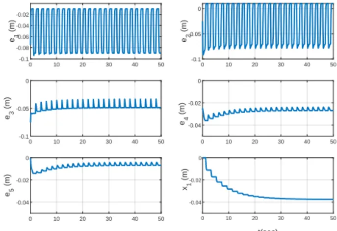
for certainw_ij they can indeed oscillate for ever. An example of such oscillations is presented in Fig. 1 for a platoon with chain sensing graph with n = 6 agents, where the initial positions arex1(0) = 0,x2(0) = 0.5,x3(0) = 1.4,x4(0) = 2.2,x5(0) = 3.1,x6(0) = 4.1, the desired distancesD21= D32 = D43 = D54 = D65 = 1 (all in meter). For the sensor disturbances we take w21 = w56 = 0, let w12 = w23=w34=w45 be a pulse signal with magnitude 0.1m, bias −0.09m, period 2 sec, and pulse width 1 sec, and let w43=w54=w65 be a pulse signal with magnitude 0.1m, bias 0.01 m, period 2 sec, and pulse width 1 sec. Finally, w32 is1sec phase delayed version of w43. The control law is that proposed in [10], i.e., (10), with

Tw¯(x) =







xif |x|>w¯+δw, 0if |x| ≤w,¯

(|x| −w)sgn(x)/δ¯ _welse,

(11) k= 3,w¯ = 0.1 m, andδ_w= 0.02 m. By comparison, Fig.

2 shows that the system does converge when the control laws (9) and (11) are used on the same initial conditions and disturbances.

C. Convergence

Theorem 5: Consider n agents 1, . . . , n, with positions x1(t), . . . , xn(t)∈Rat each time instantt, and a connected undirected sensing graphGas detailed in Section III-A. Un- der control law (9), for any class of nondecreasing functions Tw for whichTw(x) = 0if and only if |x| ≤w,

1Specifically, equation (18) in [5], which the last arguments of the proof rely on, does not hold in general, indicating again the need for convergence results based on condition (1).

0 10 20 30 40 50

-0.1 -0.08 -0.06 -0.04 -0.02

e1 (m)

0 10 20 30 40 50

-0.1 -0.05 0

e2 (m)

0 10 20 30 40 50

-0.1 -0.05 0

e3 (m)

0 10 20 30 40 50

-0.04 -0.02 0

e4 (m)

0 10 20 30 40 50

-0.04 -0.02 0

e5 (m)

0 10 20 30 40 50

t(sec)

-0.04 -0.02 0

x1 (m)

Fig. 1. Example of evolution with time of the errorsei=xi+1− xi−Di,i+1and of the position of the first agentx1for a 6 agent platoon with control laws (10) and (11) and a chain sensing graph, showing that these control laws do not guarantee convergence.

0 10 20 30 40 50

-0.5 -0.4 -0.3 -0.2 -0.1

e1 (m)

0 10 20 30 40 50

-0.2 -0.15 -0.1 -0.05 0

e2 (m)

0 10 20 30 40 50

-0.3 -0.25 -0.2 -0.15

e3 (m)

0 10 20 30 40 50

-0.2 -0.15 -0.1 -0.05 0

e4 (m)

0 10 20 30 40 50

t(sec)

-0.1 -0.05 0 0.05 0.1

e5 (m)

0 10 20 30 40 50

t(sec)

-0.4 -0.3 -0.2 -0.1 0

x1 (m)

Fig. 2. Evolution with time of the errorsei=xi+1−xi−Di,i+1

and of the position of the first agent x1 for a 6 agent platoon with control laws (9) and (11) on the same sensing graph, initial conditions and disturbances as in Fig. 2.

(a) x(t)converges :x^∗= lim_t→∞x(t)exists, and satisfies

X

j:(i,j)∈E

(x^∗_j−x^∗_i −Dji)

≤2d(i) ¯w, (12) where d(i) is the degree of agent i in G and w¯ the bound on the disturbance.

(b) For every agent iand all timet there holds pi+ min(xj(0)−pj)≤xi(t)≤pi+ max

j (xj(0)−pj) (13) Proof: Let us perform a change of variable, defining y_i=x_i−p_i. Noting that p_i−p_j=D_ij, we have

˙

yi= ˙xi=kT_{d(i) ¯w}



 X

j|(i,j)∈E

(yj−yi+wji)





=−kT_{d(i) ¯w}((Ly)i−wi), (14)

where w_i =P

j|(i,j)∈Ew_ji satisfies, |w_i| ≤ d(i) ¯w, and L is the Laplacian matrix of the graph:Lii =d(i),Lji=−1 if i and j are connected, and 0 else. By definition of T and in view of the bound |wi| ≤d(i) ¯w, y˙_i can be positive only if(Ly)_iis negative, and vice versa, so thaty(Ly)˙ _i≤0.

Moreover, It is easy to confirm thatyis absolutely continuous as it is the integral of a measurable locally bounded function.

Hence Theorem 1 shows that y converges to some y^∗ and yi(t) remains at all time in [minyi(t),maxyi(t)], which implies the convergence ofxand the inclusion (13).

We now prove that |(Ly^∗)i| ≤ 2d(i) ¯w, which implies (12), by contradiction. Suppose this condition does not hold, and without loss of generality, that (Ly^∗)i > 2d(i) ¯w.

Since y(t) converges to y^∗, there is a time t^∗ after which (Ly(t))i >2d(i) ¯w+αfor some α >0, and thus we have (Ly(t))i −wi > d(i) ¯w+α, since wi = P

j|(i,j)∈Ewij

satisfies, |wi| ≤ d(i) ¯w. Since T is non-decreasing, this means there is a time after which T_{d(i) ¯w}((Ly(t))i−wi)≥ T_{d(i) ¯w}(d(i) ¯w+α) > 0, where the last inequality follows from Td(i) ¯w(z) = 0 ⇔ |z| ≤ d(i) ¯w. As a result, y˙i would remain negative and bounded away from 0 for all timet > t^∗, in contradiction with its convergence toy^∗. Hence we must have|(Ly^∗)_i| ≤2d(i) ¯wand thus (12).

The particularization of equation (12) to the line graph implies|x^∗₂−x^∗₁−D21| ≤2 ¯wwhen applied to node 1, and

|2x^∗₂−x^∗₁−x^∗₃−D21−D32| ≤4 ¯w.

when applied to node2, so that |x^∗₃−x^∗₂−D₃₂| ≤6 ¯w. An induction argument shows then

|x^∗_k−x^∗_k−1−D_k(k−1)| ≤min (4k−6,4n−4k−2)w^∗, where the second element in the min is obtained by starting the induction from the end of the platoon.

IV. CONCLUSION

In this paper we have analyzed processes where the dynamics is not implicitly determined by (the gradient of) an energy function, but where that only serves as a barrier, leaving more freedom for the possible trajectory.

This framework beautifully matches the scenario of pla- toon formation, where the control of the dynamics has to be more conservative as it needs robustness as a priority over having an optimal configuration.

In both setups we have confirmed convergence of the processes when the energy function is quadratic described by a positive definite or Laplacian matrix. In a more general quadratic positive semi-definite case we have shown a partial concentration result, but we suspect much more is true.

These trajectory-based convergence results opens multiple perspectives: A straightforward challenge is to determine whether it is possible for a trajectory satisfying (2) to diverge or to have multiple accumulation points whenAhas rank at mostn−1 (and is not a Laplacian). Similarly, whether the absence of zero entries in the vectors of the kernel of A, required in condition (b) of Theorem 1, can be relaxed. One obvious extension to broader context is to consider more general energy functions V than quadratic ones.

Condition (2) can also be interpreted as requiring x˙ and

∇V to belong to a same cone among a finite set of cone.

This insight could be use to derive more general conditions with more general and/or position dependent cones.

REFERENCES

[1] Andrea Bacciotti and Francesca Ceragioli. Stability and stabilization of discontinuous systems and nonsmooth Lyapunov functions.ESAIM:

Control, Optimisation and Calculus of Variations, 4:361–376, 1999.

[2] John Baillieul. Remarks on a simple control law for point robot formations with exponential complexity. In Proceedings of IEEE Conference on Decision and Control, pages 357–3362, December 2006.

[3] John Baillieul and Atul Suri. Information patterns and hedging Brock- ett’s theorem in controlling vehicle formations. InProceedings of IEEE Conference on Decision and Control, pages 556–563, December 2003.

[4] Radu Balan. An extension of Barbashin-Krasovski-LaSalle theorem to a class of nonautonomous systems. arXiv preprint math/0506459, 2005.

[5] Dario Bauso, Laura Giarr´e, and Raffaele Pesenti. Consensus for networks with unknown but bounded disturbances. SIAM Journal on Control and Optimization, 48(3):1756–1770, 2009.

[6] Norman L. Biggs. Algebraic Graph Theory. Cambridge University Press, 1993.

[7] Jorge Cortes. Discontinuous dynamical systems - a tutorial on solutions, nonsmooth analysis, and stability. IEEE Control Systems Magazine, 28(3):36–73, 2008.

[8] Hanen Damak, Mohamed A. Hammami, and Boris Kalitine. On the global uniform asymptotic stability of time-varying systems. Differ- ential Equations and Dynamical Systems, 22(2):113–124, 2014.

[9] Claudio De Persis, Paolo Frasca, and Julien M. Hendrickx. Self- triggered rendezvous of gossiping second-order agents. InProceedings of IEEE Conference on Decision and Control, pages 7403–7408, December 2013.

[10] Baris Fidan and Brian D.O. Anderson. Switching control for ro- bust autonomous robot and vehicle platoon formation maintenance.

In Proceedings of 15th Mediterranean Conference on Control and Automation, pages 1–6, 2007.

[11] Mauro Franceschelli, Andrea Gasparri, Alessandro Giua, and Carla Seatzu. Decentralized estimation of Laplacian eigenvalues in multi- agent systems. Automatica, 49(4):1031–1036, 2013.

[12] Julien M. Hendrickx and John N. Tsitsiklis. A new condition for convergence in continuous-time consensus seeking systems. InPro- ceedings of IEEE Conference on Decision and Control and European Control Conference (CDC-ECC), pages 5070–5075. IEEE, 2011.

[13] Aleksandr O. Ignatyev. On the construction of the Lyapunov function with sign-definite derivative with the help of auxiliary functions with sign-constant derivatives. Journal of Mathematical Sciences, 190(4):567–588, 2013.

[14] Ali Jadbabaie, Jie Lin, and Stephen A. Morse. Coordination of groups of mobile autonomous agents using nearest neighbor rules. IEEE Transactions on Automatic Control, 48(6):988–1001, 2003.

[15] Hassan K. Khalil and Jessy W. Grizzle. Nonlinear systems. Prentice Hall, Upper Saddle River, NJ, 2002.

[16] Joseph LaSalle. Some extensions of Liapunov’s second method.IRE Transactions on Circuit Theory, 7(4):520–527, 1960.

[17] Stacy Patterson and Bassam Bamieh. Consensus and coherence in fractal networks. IEEE Transactions on Control of Network Systems, 1(4):338–348, 2014.

[18] Feyyaz Emre Sancar, Baris Fidan, and Jan P. Huissoon. Deadzone switching based cooperative adaptive cruise control with rear-end collision check. InProceeding of IEEE International Conference on Advanced Robotics, pages 283–287, 2015.

[19] N. Sreedhar. Concerning Liapunov functions for linear systems - I.

International Journal of Control, 11(1):165–171, 1970.

[20] Peter Wieland, Rodolphe Sepulchre, and Frank Allg¨ower. An internal model principle is necessary and sufficient for linear output synchro- nization.Automatica, 47(5):1068–1074, 2011.