Generating Distance Fields from Parametric Plane Curves
Gábor Valasek
Eötvös Loránd University valasek@inf.elte.hu
Submitted March 5, 2018 — Accepted September 13, 2018
Abstract
Distance fields have been presented as a general representation for both curves and surfaces [4]. Using space partitioning, adaptive distance fields (ADF) found their way into various applications, such as real-time font ren- dering [5].
Computing approximate distance fields for implicit representations and mesh objects received much attention. Parametric curves and surfaces, how- ever, are usually not part of the discussion directly. There are several algo- rithms that can be used for their conversion into distance fields. However, most of these are based converting parametric representations to piecewise linear approximations [7].
This paper presents two algorithms to directly compute distance fields from arbitrary parametric plane curves. One method is based on the rasteri- zation of general parametric curves, followed by a distance propagation using fast marching. The second proposed algorithm uses the differential geometric properties of the curve to generate simple geometric proxies, segments of os- culating circles, that are used to approximate the distance from the original curve.
Keywords:Computer Graphics, Distance Fields, Geometric Modeling MSC:65D17, 65D18, 68U07
1. Introduction
Distance fields are samples of the signed or unsigned distance function to a geomet- ric object. They are a versatile representation of curves and surfaces and have been
http://ami.uni-eszterhazy.hu
83
successfully applied in many areas of geometric modeling and computer graphics.
Distance fields can simplify otherwise sophisticated operations, such as morphing between geometries with different topologies [3], and also speed up costly queries like collision detection.
Computation of distance fields from implicit representations has been exten- sively studied in the literature [7], but direct conversion of parametric curves or surfaces is less often exposed.
This paper presents two methods to convert parametric plane curves to sampled distance fields over a uniform grid.
The first method discretizes the parametric curve to grid cells. These cells are then used to form the boundary condition of the eikonal equation that defines the signed distance function of the parametric curve. Solving this equation using fast marching results in a highly efficient, approximate solution to the distance field.
The second method uses osculating circle segments to create a piecewise circular approximation to the original curve and extracts gridpoint distances using these circle segments as proxies for the original curve. This approach provides simple means to control the trade-off between accuracy and speed of execution.
These two methods are related in that they consist of a sampling and an approx- imation step. In rasterization, we sample the continouos problem first and then compute an approximate solution. In the osculating circle scenario, first we approx- imate the original curve with continuous proxies and then sample grid distances from these entities.
2. Rasterization-based distance field generation
One of the key components in real-time computer graphics is the high speed ras- terization of geometric primitives. There are highly efficient algorithms to rasterize line segments [1], conic sections, and even higher order algebraic curves [6]. Never- theless, research on the rasterization of general parametric curves is less prominent in the literature and they are usually discussed only in terms of lower degree poly- nomials, e.g. cubic Bezier curves [2].
The first method proposed in this paper to compute the distance field of a parametric curve consists of two steps:
1. Rasterize the input curve onto the distance field grid 2. Propagate distances over the grid from the rasterized cells
Step 1 requires a robust, gap-free, as in 8-connected, discretization of the input curver(t) : [0,1]→E3. This operation is inherently representation-aware, that is, it needs to know the particular basis and control data by whichr(t)is represented.
For the sake of simplicity, we assume we are given a uniform grid, that is, a collection of rectangles of equal width and heigh. This way, the grid can be considered as collection of cells accessed by two dimensional integer indices, i.e.
Grid= [0,1, .., W−1]×[0,1, .., H−1], whereW, H∈Nare the number of colums
and rows, respectively. Rasterization should generate a gap-free subsetRasters⊂ Grid.
Step 2 starts with the cells inRastersand sets the distances to zero for these.
Then it proceeds by using the fast marching method to compute the distance of every cell fromRasters. It does not rely on any prior information about the original representation of the curve, all it requires is the set of rasterized cells and the grid onto which the distances should be propagated.
2.1. Rasterization
Letr(t) : [0,1]→E2 be a regular parametric curve, i.e. |r0(t)| 6= 0, t∈[0,1]. Let D >0 denote the common width and height of all cells, measured in the units of the space in which the curve is embeded in.
The proposed rasterization method relies on a naive, curve traversal approach:
starting from the t = 0 parameter, let us increase the parameter value by some
∆t > 0 such that we travel approximately D units along the curve, i.e. the arc length betweentandt+ ∆tis≈D. Evaluate the curve at this new point, find the closest grid cell, and if it is connected to the last cell inRasters, add its index to it as well. If the connection is broken, we have to decrease∆t until the new point on the curve is rasterized onto a cell that is connected toRasters.
To find the required ∆t > 0 change of parameter, we have to compute the inverse of the arc-length function. The arc-length function is defined as s(t) = Rt
0|r0(x)|dx: [0,1]→[0, L]and sincer(t)is regular, s(t)is strictly increasing, i.e.
it has an inverse denoted byt(l) =s−1(l) : [0, L]→[0,1].
The n-th derivative of the arc-length function can be expressed in terms of the derivatives of the curve up to n. More precisely, in the case of the first three derivatives, we have
s0(t) =|r0(t)|= (r0(t)·r0(t))12 s00(t) = (r0(t)·r0(t))120
= r0(t)·r00(t)
|r0(t)| s000(t) =
r0(t)·r00(t)
|r0(t)| 0
=r00(t)·r00(t) +r0(t)·r000(t)
|r0(t)| −(r0(t)·r00(t))2
|r0(t)|3
The above expressions can be simplified by using the Frenet coordinates of the derivatives: lett,n: [0,1]→R2denote the unit tangent and normal vectors of the curve and let xi(t) =r(i)(t)·t(t)andyi(t) =r(i)(t)·n(t). It can be easily shown that
s0(t) =x1(t), s00(t) =x2(t), s000(t) = y22(t)
x1(t)+x3(t) =κ2(t)x1(t)3+x3(t), whereκ(t)denotes the curvature function of the curve.
Let us now omit the parameter of evaluation from the formulas. Using that the derivative of the inverse function can be written as
t0= (s−1)0= 1 (s0◦s−1) t00= (s−1)00=− s00◦s−1
(s0◦s−1)3
t000= (s−1)000=−s000◦s−1·(s0◦s−1) + 3(s00◦s−1)2 (s0◦s−1)5
the derivatives of the inverse of the arc-length function can be expressed as
t0= 1 x1
, t00=−x2
x31 , t000=−(κ2x31+x3)x1−3x22
x51 =−y22+x1x3−3x22 x51 that is
t(l+ ∆l)≈t(l) + ∆l 1 x1 −∆l2
2 x2
x31−∆l3 6
y22+x3x1−3x22 x51 −...
is the Taylor expansion of t=s−1 aboutl∈[0, L].
We can compute the required∆tchange of parameter to advance approximately D units along the curve by evaluating the Taylor expansion withD
∆t=t(D) =D 1 x1 −D2
2 x2
x31−D3 6
y22+x3x1−3x22 x51 −...
Note that this means that this method is only rasterizing grid cells through which the curve passes through at leastD units long consequitively sans approxi- mation error. As a result, generally, we do not rasterize every cell that the curve touches, but the total arc-length of the curve within the omitted cells is small, provided the inverse arc-length approximation is precise enough andD is selected properly.
In practice, we have to keep track of whether the truncation introduced such an error that creates a gap during rasterization. This can be verified by comparing the integer grid coordinates of the previous and the new rasters. Should a gap occur, we can use a simple binary search betweentandt+ ∆tto find the parameter that corresponds to a curve point that rasterizes onto a grid cell that does not break the connectivity of the rasters or, better yet, until the arc-length between the two points is indeed closer toD. Using the latter as a stop criteria may or may not be possible, depending on our computational and time constraints.
2.2. Distance propogation
The second step of the algorithm can be formulated as an eikonal equation: the rasterized cells, denoted by Rasters, form the zero set of the unknown signed
distance function f(x, y)of the curve r(t), and we are looking for a solution over the entireGridsuch that
|∇f(x)|= 1 forx∈Grid f(x) = 0 forx∈Rasters
This can be solved on the grid using fast marching inO(NlogN)time [8], where N denotes the number of grids, but there are linear solvers for the problem [9].
3. Osculating cirlce-based distance field generation
The rasterization based method proves to be an efficient sequential algorithm, however, its accuracy, as shown in the test results section, may be lacking for certain applications. The method proposed in this section aims to improve on accuracy and provides a user-controllable parameter to balance between speed and precision.
The method constitutes of the following steps:
1. Adaptively sample the curve and compute osculating circles at samples 2. Select segments of the osculating circles to approximate the curve 3. Compute cell distances from osculating circle segments
Step 1 and 2 do a pre-processing of the input curve. The goal is to create a collection of circular segments as the approximation of the original curve from the osculating curcles. The number of osculating circles can be set by the user with or without taking into account the particular geometric complexity of the input curve. The more osculating circles there are, the smaller the mean and maximum error becomes, but the execution time is also increasing.
Step 3 speeds up distance computations by taking advantage of the piecewise circular structure of the curve approximant.
The following subsections discuss these three steps in detail.
3.1. Sampling the curve
In order to adapt the number of segments to the particular curve in question, one has to find a measure of complexity for parametric curves. Initially, we used the curvature function plot to determine this complexity scalar by counting the number of local extrema of the curvature function. The user could select the number of osculating circles we sample between these extrema.
However, our tests have shown that for the case of distance field computation, an equidistant parameter sampling of the curve generates roughly the same quality distance approximation as sampling the curve adapted to the curvature extrema.
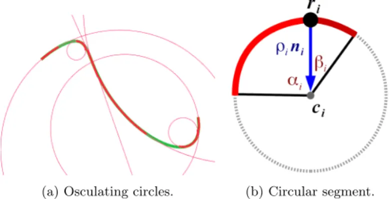
As a result, we suggest the use of equidistant parameter sampling in time critical situations. Figure 1a illustrates the osculating circles obtained by this process.
(a) Osculating circles. (b) Circular segment.
Figure 1: Osculating circles sampled along the curve (left). The representation of a single circular segment consists ofα, β >0an-
gles, associatied with the osculating curve at sampleri(right).
3.2. Determining the piecewise circular curve approximant
If all osculating circles are determined, we have to select segments on each, such that they put together form at least a globallyG0approximation to the curve.
Lett0 = 0 < t1 < t2 < ... < tN = 1 denote the selected sampling parameters along the curve. Then ri =r(ti) are the curve points and the unit tangent and normal vectors are ti = [r0(ti)]0 and ni = [(r0(ti)×r00(ti))×r0(ti)]0, respectively, where[a]0 denotes normalization, i.e. [a]0= |aa| ifa6=0.
Curvature attiis denoted byκi, their recipocals, i.e. the radii of the osculating circles areρi= κ1i, and the centers of the osculating circles areci=ri+ρini.
Since the circular segments have to includeri, we can define the segments used for approximation as two angles measured away fromni, the left angleαi and the right angleβi, see Figure 1b.
At the two endpoints we do not want to extend beyond the original curve, i.e.
α0= 0andβN = 0.
In case of a general point, consider the three osculating circles atti−1, ti, ti+1. If the (i−1)-th andi-th osculating circles intersect, letαi be the angle that cor- responds to the intersection point that is closer to ri and still lies on the left of it, i.e. on the opposite direction of ti. If the circles are non-intersecting, or the intersection lies in the opposite direction, let us pickαi such that it points to the point that is the closest to ri−12+ri. Theβi angle is determined similarly.
3.3. Distance computation
The reason for the gain in execution time lies in the fact that distance computation from a circular arc can be resolved by three point-point distance checks. We can use the distance of the point from the circular segment in the cone determined by ciand theαi, βispans, which is either|x−c|−ρior|x−c|+ρi, depending whether
x−cforms and angle less than 90 degrees withni. For points that are outside of this cone, we can check against the endpoints of the circular segments.
4. Test results
We benchmarked the execution time of both proposed algorithms and used a brute force, geometric Newton-Raphson based distance field as the ground truth for accu- racy tests. A pure Python, sequential CPU implementation was used to compare the run times. After running a batch of 1000 random curves, we obtained the runtime and accuracy statistics for the distance field generation methods. The osculating circle based method used 7 osculating circles to approximate the curve.
execution time (seconds) error
method mean std. dev. max mean std. dev.
brute force 0.36 0.03 0 0 0
raster 0.014 0.0029 30.64% 21.53% 24.65%
osculating 0.16 0.036 7.28% 0.46% 4.23%
The errors are relative errors with respect to the distance values obtained from the brute force method. Both tests were conducted on 1000 random quntic Bézier curves and the distance transform was carried out on a16×16grid.
In a sequential environment, the rasterization based approach proved to be superior, however, the accuracy suffered greatly from the initial quantization of distance values, i.e. the setting of distances to zero for rasterized cells. This, however, is necessary for most fast marching algorithms.
The accuracy (measured as mean error) of the osculating circle based approach is two orders of magnitude better than that of the rasterization method.
Another focus of our tests was to determine how does the number of osculat- ing circles correlate with the error statistics. The following table shows these as we increase the number of equidistantly sampled osculating circles. Interestingly, replacing the equidistant sampling strategy did not alter the error significantly, however, it is subject to future research to find computationally viable sample parameter selection methods that could increase distance field accuracy.
no. of circles mean error std. dev.
5 10.54% 88.86%
10 1.2% 11.95%
15 0.26% 1.79%
25 0.15% 1.4%
35 0.11% 1.08%
It is also important to note that creating a massively parallel implementation of the osculating circle based method is trivial, whereas the rasterization method suffers from the difficulties that arise when migrating fast marching to this setting, making it much harder to implement on e.g. GPUs.
Simple parallelization of the brute force method is also possible, however, one advantage of the osculating circle based method is that the actual distance trans- form part, where we measure the cell distances from the curve approximation, does not depend on the original representation of the curve, while the brute force algorithm has to rely on it throughout its execution.
5. Conclusion
This paper proposed two algorithms for the problem of direct conversion of para- metric plane curves to distance fields. We compared these methods with each other and to a brute force distance field generation algorithm.
In sequential environments, the rasterization based method proved to be the fastest. However, if accuracy is required, the osculating circle based approach offers a superior solution. It relies on the prior knowledge of the representation of the curve, even though to a lesser extent than the brute force approach, which has to be taken into account when it comes to implementation.
References
[1] J. E. Bresenham: Algorithm for computer control of a digital plotter, IBM Systems Journal, Volume 4 Issue 1, March 1965, Pages 25-30
[2] S.-L. Chang, M. S. R. Rocchetti: Rendering cubic curves and surfaces with integer adaptive forward differencing, SIGGRAPH ’89 Proceedings of the 16th annual conference on Computer graphics and interactive techniques, Pages 157 - 166, ISBN:0- 89791-312-4
[3] D. Cohen-Or , D. Levin , A. Solomovici: Three-Dimensional Distance Field Metamorphosis,ACM TRANSACTIONS ON GRAPHICS 1998, Volume 17, Number 2, Pages 116–141
[4] Sarah F. Frisken, Ronald N. Perry, Alyn P. Rockwood, Thouis R. Jones:
Adaptively sampled distance fields: a general representation of shape for computer graphics, Proceeding SIGGRAPH ’00 Proceedings of the 27th annual conference on Computer graphics and interactive techniques 2000, Pages 249-254
[5] C. Green: Improved Alpha-Tested Magnification for Vector Textures and Special Effects, Proceeding SIGGRAPH ’07 ACM SIGGRAPH 2007 courses, 2007, pages 9–
18.
[6] J. D. Hobby: Rasterization of nonparametric curves, ACM Transactions on Graphics, Volume 9 Issue 3, July 1990, Pages 262-277
[7] Mark W. Jones, J. Andreas Baerentzen, Milos Sramek: 3D Distance Fields:
A Survey of Techniques and Applications, IEEE Transactions on Visualization and Computer Graphics, Volume 12 Issue 4, July 2006, Page 581-599
[8] J.A. Sethian: A Fast Marching Level Set Method for Monotonically Advancing Fronts, Proc. Nat. Acad. Sci., 93, 4, pp.1591-1595, 1996.
[9] L. Yatziv, A. Bartesaghi, G. Sapiro: O(N) implementation of the fast marching algorithm, Journal of Computational Physics, Volume 212, Issue 2, 1 March 2006, Pages 393-399