SELF-ORGANIZED CRITICALITY OF THE BRAIN: FRACTAL ANALYSIS OF THE HUMAN SLEEP EEG

(1)

SELF-ORGANIZED CRITICALITY OF THE BRAIN:

FRACTAL ANALYSIS OF THE HUMAN SLEEP EEG

Ph.D. dissertation

Béla Weiss

Supervisor:

Tamás Roska, D.Sc.

ordinary member of the Hungarian Academy of Sciences Scientific advisers:

György Karmos, M.D., Ph.D.

emeritus professor and

Zsuzsanna Vágó, Ph.D.

associate professor

Pázmány Péter Catholic University Faculty of Information Technology

Interdisciplinary Technical Sciences Doctoral School

Budapest, 2010

(2)

(3)

To the memory of my Parents and Grandparents.

(4)

(5)

Acknowledgment

First and foremost, I would like to thank the consistent support of my supervisor and head of the doctoral school, Prof. Tamás Roska. The interdisciplinary environment that he provided turned out to be of a crucial importance for my research.

I would also like to express my gratitude to my advisers, Prof. György Karmos and Zsuzsanna Vágó for sharing their concerns and suggestions related to physiological and mathematical aspects of my work. I am indebted to Prof. Ronald Tetzlaff for his tutoring during my stay at the Institute of Applied Physics, Johann Wolfgang Goethe University in Frankfurt, Germany (IAP). During all these years my research was helped by Prof.

Péter Halász and I appreciate this really much.

I am also thankful to my closest collaborators who contributed to my work. I am very grateful to Zsófia Clemens for all those discussions and her useful advices. I also acknowledge the contribution of Róbert Bódizs. Without the recordings acquired in his laboratory this research would not be possible. Although my work related to epilepsy did not become a part of the dissertation I thank the whole epilepsy monitoring and surgery team at the National Institute of Neuroscience. Special thanks go to István Ulbert, Lóránd Er ss, László Entz, Rita Jakus and Dániel Fabó.

I am also very grateful to my fellow PhD students, especially to Éva Bankó, Csaba Benedek, Mária Ercsey-Ravasz, Gergely Feldhoffer, László Füredi, Gaurav Gandhi, András Kiss, Giovanni Pazienza, Tamás Pilissy, Gergely Soós, Ákos Tar, Róbert Tibold, Dávid Tisza, Gergely Treplán, József Veres and Péter Vizi for all their help, fruitful discussions and the time we spent together. I especially thank György Cserey, Zoltán Fodróczi, Viktor Gál, Kristóf Iván, Kristóf Karacs, Attila Kis, András Oláh and Róbert Wagner for their help at the beginning of my PhD studies.

I also say thank to all my colleagues at the IAP, but especially to Denis Dzafic, Martin Eichler, Gunter Geis, Frank Gollas, Leonardo Nicolosi, Christian Niederhöfer and Hermine Reichau for their friendship and help during my stay in Germany.

I acknowledge the kind help of Anna Csókási, Lívia Adorján, Judit Tihanyi, Vida Tivadarné Katinka and the personnel of the Students’ Office, the Dean’s Office, the Warden’s Office, the Financial Department, the IT Department, the Library, the Reception and the cleaning personnel.

I thank all my friends for being so patient during my busy days.

(6)

I am tremendously grateful to my Parents and Grandparents for all their love and support. Special thanks go to Ómama for her fostering and endless love and to my sister Ági and her family for their help during the toughest years.

Finally, I would like to thank my wife Nóra for her love, support, patient and understanding.

(7)

SUMMARY OF ABBREVIATIONS

Abbreviation Concept

AN adaptive neuro-fuzzy inference system ANOVA analysis of variance

ave unweighted average distance (linkage method) CCC cophenet correlation coefficient

cen centroid distance (linkage method) che Chebychev distance (similarity measure) cit city block metric (similarity measure) CMS selection of channel x measure features com furthest distance (linkage method) cor correlation distance (similarity measure) cos cosine distance (similarity measure)

CS selection of channels considering a same measure CVT cross-validation time

DFA detrended fluctuation analysis

ECG electrocardiogram

EEG electroencephalogram

EMG electromyogram

EOG electrooculogram

euc Euclidean distance (similarity measure) FF feedforward neural network

FFT fast Fourier transform FST feature selection time

IEEG intracranial electroencephalogram LD linear discriminant analysis

LS support vector machine with a linear kernel function mah Mahalanobis distance (similarity measure)

MANOVA multivariate ANOVA

med weighted center of mass distance (linkage method)

(10)

min Minkowski metric (similarity measure) MLR multiple linear regression

MS selection of measures considering a same channel NB naïve Bayes classifier

OA overall accuracy

PN probabilistic neural network PSM power spectral measure

QD quadratic discriminant analysis RB radial basis function neural network RBP relative band power

RS support vector machine with a radial basis kernel function seu standardized Euclidean distance (similarity measure) SFFS sequential forward feature selection

sin shortest distance (linkage method)

SO slow oscillation

SOC self-organized criticality SVM support vector machine

war inner squared distance (linkage method) wei weighted average distance (linkage method)

(11)

C h a p t e r O n e

INTRODUCTION

1.1. Preface

Despite of the broad spectrum of electrophysiological and imaging methods available in the field of neurobiology still little is known about how exactly complex neural dynamics emerge. Hopefully, application of novel theoretical approaches and computational methods aimed for analysis and modeling of complex systems might provide a deeper insight into physiological and pathological mechanisms of the brain.

With advent of relatively cheap and high performance personal computers sophisticated and computation demanding time series analysis methods became available to a broad brain research community. Application of chaos theory and non-linear time series methods gave a deeper insight into brain dynamics reflected by EEG signals. For a comprehensive recent review on non-linear analysis of EEG I refer to [16]. This approach relies on a transition from the time domain to the phase space and generation of trajectories for EEG time series using different embedding techniques. Inferences about brain dynamics were drawn by estimating different characteristics of trajectory attractors using measures such as the correlation dimension D2, the fractal dimension Df, the largest Lyapunov exponent L1, etc. Early results were promising and suggested a deterministic nature of brain dynamics with a rather low-dimensional chaotic behavior in physiological and pathological conditions that could not be revealed using simple linear methods such as the power spectral analyses. Filtered noise, however, can mimic the signatures of deterministic chaos [17]. This latter finding necessitated a revision of results obtained by non-linear techniques. Surrogate data analyses [18] did not entirely support early results on the low-dimensional chaotic behavior of the brain. This was in agreement with the finding that the relatively high complexity of the EEG signals does not allow a reliable dissociation of its waxing and waning oscillations exceeding 2-15 s from that of the filtered white noise [19-21]. As a consequence alternative approaches were developed including novel non-linear and stochastic time series analysis methods.

Unlike deterministic approaches aimed at finding low-dimensional chaos, the self- organized criticality (SOC) framework allows for describing the high-dimensional character of the dynamics and the presence of stochastic effects [22]. SOC is a

(12)

phenomenon characterizing systems that might arrive at a critical state (phase transition) without any tuning of a specific parameter [23]. The proof of presence of SOC requires a demonstration of spatio-temporal long-range correlations and power-law scale-free (also called self-similar or fractal) fluctuations [24]. Scale-free behavior means that no characteristic scales dominate the dynamics of the underlying processes. It also reflects a tendency of complex systems to develop correlations that decay more slowly and extend over larger distances in time and space than the mechanisms of the underlying processes would suggest [24-26]. The long-range correlations build up through local interactions until they extend throughout the entire system. After this stage, the dynamics of the system exhibit power-law scaling behavior and the underlying process operates in a critical state [23, 27].

Several features of neural networks are consistent with SOC, such as a large number of elements (neurons) interacting with each other in a nonlinear way (e.g. presence of threshold for spiking), a possibility to change and save connectivity between the elements (e.g. via synaptic plasticity), absence of any special parameter tuning, and spatio-temporal dynamics obeying power-law statistics [22, 28]. A critical state is a regime of a system where opposing forces are balanced. In the nervous system such a balance might be represented by the relationship between excitation and inhibition, which is known to be important for the transfer of information [29] and for the sustained neuronal activity [30]. Neural network simulations demonstrated that the presence of long-range spatio-temporal correlations is beneficial for the optimal transfer of information since these correlations represent an optimal compromise between high susceptibility to perturbations and stability in the system [31, 32].

All these properties of the brain suggest that the SOC paradigm might be an appropriate tool to investigate and model of neural activities. In line with this fractal geometry of brain structures [33, 34] as well as power-law spatio-temporal properties of neuronal activities have been revealed. Although the spatial power spectral density (PSDx) of scalp EEG recordings might deviate from the ideal power-law scale-free behavior [35], the PSDx of epipial EEG conforms to it [36]. Temporal long-range correlations were observed at different levels of the brain electrical activity hierarchy in different species and during different conditions. For example, Lowen et al. revealed that the individual ion channel currents show long-term correlation and possess fractal properties [37].

Considering spike trains in extracellular recordings, long-term correlations were found among interspike intervals of the medullary sympathetic neurons in cats [38]. Spasic et

(13)

al. showed that the fractal dimension of local field potentials of anaesthetized rats changes significantly after unilateral discrete injury [39]. Fractal exponent of EEG activity in the Gallotia galloti lizard decreased with the increment of temperature from 25

°C to 35 °C [40].

1.2. Motivation and aims

Overall, the motivation of my research is two-fold and the work that I have done may be related to different general steps of brain research (Figure 1.1). From the theoretical point of view I am interested in how complex neural dynamics emerge across different scales and how are these dynamics related to different physiological and pathological mechanisms that thoroughly affect the information sensation, processing, storage and retrieval of the brain. On the other hand, I am interested in practical aspects of brain research as well. Namely, as an engineer I am also motivated to reveal how biologically- inspired information processing models can be transferred into technical applications, including the control of the brain itself. At the confluence of my general research interests I found the investigation of vigilance level and epilepsy to be of a crucial importance given the well-known influence of these basic mechanisms on the information processing properties of the brain. Thus, I devoted my PhD student years to explore the capability of the SOC paradigm to describe the information processing properties of the brain by fractal analyses of physiological sleep and epileptic neural activities. However, due to the size limitations of the dissertation and the difficulties related to the analyses of epileptic activities I will here concentrate on presentation of my results related to fractal analysis of the human sleep EEG only. To draw inferences about fractal properties of the brain activity I assessed topographic and sleep stage-wise distribution of monofractal and multifractal EEG features and the relation of these measures with power spectral properties. With a more practical motivation in the background I assessed whether a combination of fractal and power spectral EEG features

Figure 1.1. A possible process diagram of brain analyses and intervention.

(14)

might improve the classification of the vigilance state.

1.3. Framework of the dissertation

In Chapter 2, a general description of materials and methods that have been used during the investigations is provided. Methods related to specific parts of the research will be provided in the corresponding chapters.

In Chapter 3, topographic and sleep stage-wise distribution of monofractal and multifractal sleep EEG measures and their relation to power spectral measures are assessed.

In Chapter 4, sleep stage discrimination capability of fractal and power spectral measures of EEG signals recorded at different topographic locations was analyzed with a special regard to combination of different features.

Conclusions are given in Chapter 5.

Summary of the new scientific results in form of thesis and delineation of possible applications can be found in Chapter 6.

Chapter 7 contains appendices.

1.3.1. General notes

From now on (except of Chapter 6) I will use “We/we” instead of “I” since most of the research was carried out in collaboration.

Although the notations used within a single chapter are unique, the same symbol may denote diverse quantities in two different chapters.

(15)

C h a p t e r T w o

MATERIALS AND METHODS

2.1. Subjects and EEG recordings

Twenty-two healthy subjects with no sleep disturbances, free of drugs and medications as assessed by an interview and questionnaires on sleeping habits and health participated in the study (age: 17–55 years, mean±S.D.: 31±9 years, 11 males and 11 females). The study was approved by the ethical committee of the Semmelweis University and subjects gave written informed consent to participation. Sleep was recorded in the sleep laboratory for two consecutive nights. The present study was based on the second night.

The timing of lights off was determined by the subjects, and morning awakenings were spontaneous. On average subjects spent 462.39±69.01 (mean±S.D.) minutes in sleep.

Sleep was recorded by standard polysomnography, including electroencephalography (Fp1, Fp2, F3, F4, Fz, F7, F8, C3, C4, Cz, P3, P4, T3, T4, T5, T6, O1 and O2 electrodes), electrooculography (EOG), bipolar submental electromyography (EMG) and electrocardiography (ECG). EEG electrodes were referenced to the contralateral mastoid.

Midline EEG electrodes were referenced to the right mastoid. Impedance of the EEG electrodes was kept below 5 k . Signals were collected, pre-filtered, amplified and digitized at a sampling rate of f_s =249 Hz using the 30 channel Flat Style SLEEP La Mont Headbox with implemented second order filters at 0.5 Hz (high pass) and 70 Hz (low pass) as well as the HBX32-SLP 32 channel preamplifier (La Mont Medical Inc., USA). Additionally, a 50 Hz digital notch filtering was performed by means of the DataLab acquisition software (Medcare, Iceland).

2.2. EEG processing

Pre-processing and feature estimation were accomplished in a self-developed EEG visualization and processing toolbox under Matlab2009b (MathWorks, Natick, MA, USA). This toolbox is freely available under GNU license upon request [41].

Calculations were performed on different hardware configurations and operating systems. Computation times presented later stand for the following configuration: Linux operating system; Intel Xeon 64 bit 3 GHz CPU with 8 cores, 2 MB cache memory; 2

(16)

GB RAM memory. Statistical analyses were performed using STATISTICA (StatSoft, Inc., Tulsa, OK, USA) and Matlab2009b.

2.2.1. Pre-processing

Although hardware filtering had been applied during EEG recording, some artifacts remained. Thus, we first performed software filtering on the raw EEG recordings with Butterworth IIR filters (eight order 0.3 Hz-70 Hz band-pass and 50 Hz notch with a quality factor Q=45). To avoid phase distortion, we used the built-in filtfilt() function of the Matlab for zero-phase digital filtering.

For all subjects a hypnogram was prepared according to the Rechtschaffen and Kales standard [15] using 20 s long epochs. To compare the analyzed EEG features during different sleep stages 90 epochs of 20 s length were selected from sleep stages NREM2, NREM4 and REM (30 minutes/stage) for all subjects. Selection included segments without artifact contamination only.

2.2.2. Fractal analysis

Monofractal and multifractal properties of the selected EEG epochs were evaluated by estimation of the self-similarity parameter H (also called Hurst exponent or Hurst parameter) [42, 43] and the range of fractal spectra ( D) [44], respectively. To estimate H, we applied the rescaled adjusted range based approach, while D was approximated by estimation of generalized dimensions spectra. The brief description of the applied methods can be found in the following subsections.

2.2.2.1.Estimation of the Hurst exponent

The stochastic process ^{X t}

( )

with continuous parameter t is self-similar with the self- similarity parameter H if the distribution of the rescaled process ^{c X ct}⁻^H

( )

is the same as the distribution of ^{X t}

( )

^{, where} ^c^>⁰ is arbitrary [43]. H is widely used to assess monofractality, scale-free properties and the degree of long-range temporal correlations of time series. When 0<H<0.5, an increase in the process is more probably followed by a decrease (anti-persistence) and vice-versa, the process is considered to have short- range dependence. If H =0.5, observations of the process are uncorrelated. When

0.5<H <1, an increase in the process is more probably followed by an increase and a

(17)

decrease is more probably followed by a decrease (persistence), the process is considered to have long-range dependence [42, 43, 45-47].

Basically two kinds of homogenous self-similar signals exist: fractional Gaussian noises (fGn) and fractional Brownian motions (fBm). fGn processes are considered to be stationary with a constant mean value and constant variance over time, while fBm’s exhibit non-stationary property with a time-dependent variance. fGn and fBm signals are interconvertible. Taking the differences between neighboring elements of an fBm time series one might create an fGn signal, while by cumulative summation of fGn elements one can generate a motion process. The corresponding fBm and fGn signals are characterized by the same H. Self-similarity of a time series is also reflected in their power spectrum. The power versus frequency relationship is given by ^{P f}

( )

^∝ ^f⁻^κ^,

where is called spectral or fractal exponent. Depending on the type of a fractal signal the relationship between H and is given by ^H ⁼

(

^κ⁺^{1 2, 1}

)

^{− <}^κ^<¹ for fGn and

(

^{1 2 , 1}

)

³

H = κ− <κ < for fBm. Similarly, H is linearly related to the detrended fluctuation analysis (DFA) exponent [48, 49] as H =λ for fGn signals and H =λ−1 in case of fBm processes. Additionally, the Hurst exponent is also related to the widely used fractal dimension as H = −2 D_f for fBm time series [50, 51]. Although many approaches are available for the estimation of H none of these can be generally considered as an ideal one because of differences of fGn and fBm signals [50, 52-54] and doubts related to the estimation of non-linear parameters from time series of finite length [47, 55-59]. For the estimation of H we used the rescaled adjusted range or R S statistics based method [42, 43, 45]. We implemented this method keeping in mind the stationarity properties of the analyzed EEG segments and the fact that this method is applicable to stationary fGn processes or to differenced fBm signals only.

Here we provide a short description of this approach. Let ^{X n}

( )

be a discrete time series.

The partial sum process is defined as

( ) ( )

1

, .

n

i

Y n X i n

=

= ∈ (2.1)

The sample variance of the process X can be obtained using

( ) ( ) ( )

2 2

1

1 1

.

n

i

S n X i Y n

n = n

= − (2.2)

(18)

The adjusted range is given by

( ) ( ) ( )

1

max1 min ,

i n

R n i n i i

≤ ≤

= ≤ ≤ ∆ − ∆ (2.3)

where

( ) ( )

^Y

( )

ⁿ^.

n i i Y

i = −

∆ (2.4)

The R S statistics or the rescaled adjusted range is defined by

( ) ( ) ( )

^.

R S n =R n S n (2.5)

In [43] it was proven that for self-similar processes the expected value of ^{R S n}

( )

^is

proportional to n^H, i.e.

[ ( ) ]

^~^CH ^,

nH

n S R

E (2.6)

as n→ ∞, where C_H is a positive constant and H is the self-similarity parameter of the process. Using this power-law relationship the Hurst exponent can be estimated by:

[ ( ) ]

⁾ ^log

( )

^.

log(

~ E R S n n

H (2.7)

To estimate H, the N sample point long data segments (N =20 249∗ =4980) were subdivided into K blocks (K =20). Blocks of length N K corresponded to duration of 1 second. ^{R S n}

( )

was computed starting at points k_l =lN K+1, l =0,1,...,K −1. These values can be denoted by R k n S k n

(

l^,

) (

l^,

)

. Overlapping of blocks was avoided, the upper boundary, i.e., the high cut-off point (hcf =249) of n was limited to N K. This resulted K different estimates of ^{R n S n}

( ) ( )

for each value of lag n. By plotting

( ) ( )

log R k n S k n_l, _l, versus ^log

( )

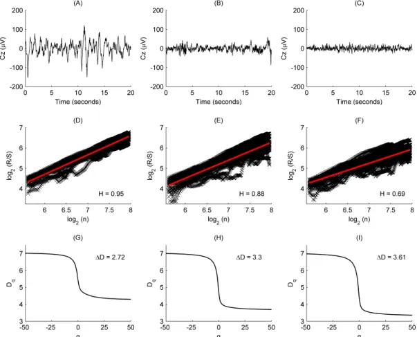
ⁿ we got the so-called pox plot for the R S statistics. H can be estimated by fitting a straight line to the points in this plot. H is equal to the slope of the fitted line. Pox plots for 20s long representative brain electrical activities recorded from subject #16 (channel Cz) during sleep stages NREM4, NREM2 and REM can be seen in Figure 2.1. Due to the transient zone at the low end of the plot we set a low cut-off point as well. The low cut-off point (lcf =50) was ~20% of N K. Thus, we used only values of n that lie between the low and high cut-off points to estimate H. This range of n (lcf ~ 0.2 , s hcf ~ 1 s) was in agreement with the scaling range [0.2 s 1 s] used for estimation of DFA -exponents in [60]. Hereby our estimations

(19)

were not influenced by the frequency cut-offs of the applied 0.3Hz-70Hz or (3.333s)^-1- (0.014s)^-1 band-pass filter. The computation of a single H value took about 1.8 s with these particular settings.

2.2.2.2.Estimation of multifractal spectra

Homogenous self-similar time series can be described by a single scale-free exponent.

These signals are also called monofractal time series. Additionally, heterogeneous multifractal time series showing self-similarity only in local ranges of the structure also exist. Their scale-free property varies in time. Hence they should be decomposed into many sub-sets and characterized by different exponents. This can be carried out by estimation of fractal spectra. Using the Alfréd Rényi’s generalized entropy, a continuous spectrum of generalized dimensions (also called Rényi dimensions or fractal spectrum)

Figure 2.1. (A-C) Examples of EEG segments recorded from subject #16 during sleep stages NREM4 (A), NREM2 (B) and REM (C). (D-F) Pox plots of the R S statistics and the estimated H values for the EEG segments presented in the top row (D: NREM4; E: NREM2; F: REM). (G-I) Generalized dimension spectra and the estimated D values for the EEG segments presented in the top row (G: NREM4; H:

NREM2; I: REM).

(20)

Dq can be defined, where −∞ ≤q≤ ∞ [61]. A common method for estimation of fractal spectra is the box-counting technique. In this study we applied a box-counting approach that is based on estimation of the moments of signal amplitude distribution and was also used in [44]. One reason for choosing this method is that a previous study [62] revealed a promising sleep stage classification performance based on the entropy of amplitudes (ENA), a measure that is closely related to the amplitude distribution of time series. In our case Dq is defined as follows:

( )

0

log ,

lim , 1.

1 log

q V

D q V q

q V

δ

χ δ δ

= → ≠

− (2.8)

δV is the bin width or box length (set to 0.3 V in this case based on the conversion range and the resolution of the analogue to digital converter). The partition function can be obtained using

( )

⁽ ⁾

( )

1

, , ,

b V i i

q V q V

δ

χ δ χ δ

=

= (2.9)

where ^{b V}

(

^δ

)

denotes the number of non-overlapping bins

( )

^V^max ^V^min ^.

b Vδ V

δ

= − (2.10)

Vmax and V_min are the maximum and minimum values of EEG signals recorded during measurements, respectively. χi

(

q V^,δ

)

= pi^q is a weighted measure that represents the percentage of EEG values that falls into the ith bin, and q is the moment or weight of the measure. If n_i is the number of EEG values in the ith bin and N is the total number of the samples, than the probability that the signal falls into the ith bin of length Vδ is:

i .

i

p n

= N (2.11)

Some of the Dq values are known under different names and widely used in the field of time series analysis. D0 is the Hausdorff-Besicovitch or fractal dimension. For q=1 one should use

( )

1

1 0

log

lim ,

log 1

b V

i i

i V

p p

D V

δ

δ δ

=

→

−

= (2.12)

(21)

where the numerator is the well-known Shannon’s entropy and can be related to ENA applied in [62]. D2 is called correlation dimension.

The range of fractal spectra is defined as ^∆^D⁼^max

( )

^D^q ⁻^min

( )

^D^q ^{, where}

( )

max D_q =D_−∞, ^min

( )

^D^q ⁼^D^∞^{, i.e.,} ^∆^{D D}⁼ ^−∞⁻^D^∞^{, since} ^D^q is a monotonically decreasing function. D is a measure of multifractality, indicates deviation from monofractal. Larger D indicates multifractality, while smaller D indicates that the analyzed system tends to possess the monofractal property. We estimated the range values by ∆D D= ₋₅₀−D₅₀ based on preliminary analysis (Fig. 2). The approximation of a single D value took about 2.4 ms with these particular settings.

2.2.3. Power spectral measures (PSMs)

To assess the relationship between fractal measures and power spectral properties of sleep EEG signals, we estimated the relative power of widely used frequency bands (RBPs). Relative powers were used instead of absolute ones in order to avoid the effect of variation of total power across subjects. To describe spectral properties in a more compact way, we calculated the spectral edge frequency (fse) since this measure can be considered as a clinically well-established EEG measure for monitoring sleep cycles and depth of anesthesia [62-65].

Before estimation of power spectral EEG features, Hanning windowing was applied to the selected epochs to damp out the frequency leakage, i.e. the Gibbs phenomenon that originates from truncation of time series. From these windowed time series the power spectra ^{P f}

( )

were obtained using the Fast Fourier Transformation (FFT) with frequency resolution ∆ =f 0.152 Hz and range

[

^{0 Hz,}fs ^{2 Hz}

]

. The relative power of the B frequency band can be calculated from a power spectrum as follows:

( ) ( )

1

,

ub

lb B

i B i B

Br N

T i

i

P P f

P P

P f

=

= = (2.13)

where PT is the total power of the time series, PB is the total power of the B frequency band, fi =

(

i−¹

)

∆f with a maximal value of f_s 2 when i=N, Bub and Blb are indices corresponding to the upper and lower boundary frequencies of the B band, respectively.

The analyzed bands were as follows: SO: (0.5-1] Hz, : (1-4] Hz, : (4-8] Hz, : (8-11]

(22)

Hz, : (11-16] Hz, : (16-30] Hz, : (30-70] Hz. These frequency bands are thought to represent specific EEG patterns. Slow oscillations (SOs) were assessed separately from delta band activity given their distinct characteristics [66, 67].

The spectral edge frequency was defined as the frequency up to which SEP % of the total power of the

[

^{0 Hz,}fcse^Hz

]

frequency range is accumulated:

( ) ( )

0 0

100 .

se cse

f f

P f df =SEP P f df (2.14)

In this study SEP and cut-off fcse frequency parameters were set to 95 % and 70 Hz, respectively. According to Eq. (2.14) and the nature of sleep EEG, lower fse values can be predicted for deeper sleep stages since during these states the power spectrum is biased towards lower frequencies.

Calculation of power spectra and their parameters can be realized almost real-time using the FFT algorithm with appropriate settings and hardware architecture.

(23)

C h a p t e r T h r e e

FRACTAL PROPERTIES OF THE HUMAN SLEEP EEG AND THEIR RELATIONS TO POWER SPECTRAL MEASURES

3.1. Introduction

The exact values of fractal measures may be related to biophysical mechanisms and the neural architecture underlying oscillations [22], however, given the uncertainties related to the estimation of these measures [47, 55-59] it might be more reasonable to compare the variances of features for different conditions. In line with this, a series of human studies revealed differences in the fractal measures between specific conditions. For example Linkenkaer-Hansen et al. showed that mu and alpha oscillations scale similarly, but beta oscillations have a significantly smaller scaling exponent compared to these two latter oscillations during eyes-closed state [22]. Another study showed that long-range temporal correlations are stronger in the eyes-closed condition as compared with the eyes-open condition [68]. In the study of Nikulin and Brismar largest exponent values for alpha and beta oscillations were found during the eyes-closed condition in the occipital and parietal areas [28]. Fractal dimension was found to be significantly higher for drowsy EEG compared to the wake state [69]. Increased sensory input [70] or high level of alertness [71] was shown to disrupt long-range temporal correlations. Several studies also addressed self-similarity of sleep EEG [46, 60, 72-76]. Generally, most of these studies reported higher scaling exponents and thus stronger long-range temporal correlations for deeper sleep stages. However, these studies were limited by a low sampling rate (100Hz in [46, 73-75]; 128Hz in [60]) or a low number of EEG channels (Fpz-Cz and Pz-Cz in [46, 75]; Cz in [73, 74]; C3 in [60, 76]; C4 in [72]). Furthermore, in contrast to the general opinion that the EEG is more regular and synchronized during deeper sleep stages, the only study that assessed multifractality of the sleep EEG found that the EEG is most multifractal during NREM3 and NREM4. It is to be noted that none of the abovementioned sleep studies assessed topographic aspects of the temporal fractal properties. Moreover, as far as we know, no previous study carried out a joint analysis of monofractal and multifractal properties, neither the relationship between fractal and power spectral measures was assessed yet. Therefore, in this study we attempted to address these theoretical controversies and shortcomings by estimation of spatial and

(24)

sleep stage-wise distributions of temporal monofractal and multifractal properties of the human sleep EEG and by assessing the relation of fractal measures with power spectral properties. Our analyses included: comparison of inter-site correlations, estimations of cross-correlations between monofractal and multifractal measures as well as between fractal and power spectral measures, multiple linear regression analysis, hierarchical clustering of the EEG channels and measures, assessment of gender-related differences of particular measures.

3.2. Methods

3.2.1. Recordings and estimated measures

All analyses except of the assessment of gender-related differences were carried out using the recordings of 22 subjects introduced in the previous chapter. Gender analysis was carried out using recordings of 17 subjects only. Nine female (age: 25–37 years, mean±S.D.: 29.1±3.9 years) and eight male (age: 24–37 years, mean±S.D.: 30.5±4.2 years) healthy young adults were selected from the database to form male and female groups with similar case numbers and similar age characteristics (mean, range and S.D.).

Monofractal and multifractal properties of the selected EEG epochs were evaluated by estimation of the self-similarity parameter H and the range of fractal spectra ( D), respectively. Power spectral properties of the human sleep EEG were assessed by calculating relative band powers and the spectral edge frequency. Detailed description of estimation settings can be found in the previous chapter. Additionally, we estimated the multifractal measures for the whole-night EEG recording with 19 s overlap of the 20 s long epochs to reveal general tendencies of the measures across different sleep stages. To emphasize slower dynamics and suppress promiscuous perturbations that can occur due to artefacts we applied moving average to the whole-night courses of the measures.

Moving average of the ^{X i}

( )

discrete time series with a 2a+1, a=1, 2,... long sliding window was defined as:

( )

¹

( )

^.

2 1

i a

j i a

MA i X j

a

+

= −

= + (3.1)

The value of parameter a was set to 45 for visualization purposes, depicting this way averages of 91 estimated values of H and D.

(25)

3.2.2. Statistical analysis

3.2.2.1.Topographic distribution of EEG measures across different sleep stages At the individual level comparisons between sleep stages relied on the selected 3x90 epochs of 20 s length. To test whether the fractal variables H and D are both together affected by the sleep stages, first we performed one-way multivariate analysis of variance (MANOVA). The independent variable “STAGE” contained groups NREM4, NREM2 and REM. Afterwards, to identify the specific dependent variables that contributed to the significant overall effect, one-way ANOVA test was applied to both dependent variables (H and D). Since ANOVA revealed significant main effects for both H and D, Tukey HSD post-hoc test was used for pair-wise comparison of group means. All statistical tests were carried out for all channels separately.

At the group level statistical analyses were carried out using individual medians of fractal and power spectral measures. Normality of the estimated features was tested using the Shapiro-Wilk W test, while the homogeneity of variances was evaluated with the Levene test. Since not all of the estimated measures matched normality and homogeneity in each channel we evaluated the effect of sleep stages using the non-parametric one-way Kruskal-Wallis ANOVA. Individual medians of the estimated measures were grouped using the independent variable “STAGE” having the same factors levels as in the case of individual-level analyses (NREM4, NREM2 and REM). Pair-wise comparison of sleep stages was carried out with rank post-hoc test. To test differences between bilateral symmetric scalp locations we used the Wilcoxon matched pairs test for each measure and sleep stage. For this purpose eight symmetrical channel pairs (Fp1-Fp2, F7-F8, F3-F4, C3-C4, T3-T4, T5-T6, P3-P4, O1-O2) and an additional midline channel pair (Fz-Cz) were formed.

3.2.2.2.Cross-correlation analysis

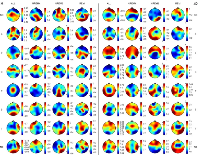
Cross-correlations were calculated between locations for all estimated measures (inter- site correlations) and between the measures at each location. Specifically, cross- correlations were carried out between monofractal and multifractal measures as well as between fractal and power spectral features. Spearman’s correlation coefficients were calculated in all cases using individual medians of particular EEG measures. Sleep stages were considered separately as well as together. To assess the contribution of specific frequency band activities to the compact measures (H, D and fse) we used multiple linear regression analysis.

(26)

3.2.2.3.Hierarchical clustering

Effect of topography was analyzed by hierarchical clustering of channels for all three sleep stages. Z-score standardization of the individual medians was carried out for all measures and channels separately. Hierarchical channel cluster trees were generated by pairing eight similarity measures (Euclidean distance (euc); standardized Euclidean distance (seu); Mahalanobis distance (mah); city block metric (cit); Minkowski metric (min); cosine distance (cos); correlation distance (cor); Chebychev distance (che)) with seven linkage methods (unweighted average distance (ave); centroid distance (cen);

furthest distance (com); weighted center of mass distance (med); shortest distance (sin);

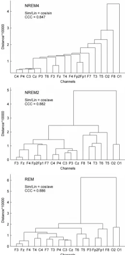
inner squared distance (war); weighted average distance (wei)). Performance of each combination was assessed by calculation of the cophenet correlation coefficient (CCC).

We selected the similarity-linkage pair with highest CCC value to cluster the channels into four and nine clusters. The 4-cluster analysis was aimed to reveal possible groupings of neighbor EEG channels and thus forming e.g. anterior, posterior, central, lateral or similar clusters. The 9-cluster analysis was applied to assess whether symmetrical EEG channels (see section 3.2.2.1) also cluster together.

Clustergrams were generated for measure and channel clustering using group-level medians (medians of individual medians) of all measures in all channels. Standardization of features was performed across channels. Clustergrams, enclosing heat maps and dendrograms were examined for sleep stages separately. Hierarchical channel cluster trees were generated using the cosine similarity metric and the unweighted average linkage method. Measure dendrograms were constructed applying the Euclidean distance as a similarity measure and the unweighted average method for linkage. Channel clustering was also carried out based on the two fractal measures as well as combining the seven relative band powers.

3.2.2.4.Effects of gender

Normality of the estimated features was tested using the Shapiro-Wilk W test. Since not all of the estimated measures matched normality in each channel the effect of gender was assessed by the Mann-Whitney U test. Individual medians of all features in all channels and during all three sleep stages were compared separately according to the “GENDER”

factor.

(27)

3.3. Results

3.3.1. Distribution of EEG measures across vigilance states and topographic locations

Since results found at the individual level were near similar across subjects here we restrict presentation of individual data to a representative subject (#16). Inspection of individual whole-night H and D profiles and corresponding hypnograms in this subject indicated a visually striking correlation with the succession of sleep cycles. As can be seen in Figure 3.1, as sleep deepens H increases and D decreases while with sleep shallowing H and D exhibit an inverse course. In Figure 3.2 H and D measures are shown with an expanded time scale for a single sleep cycle that contains a typical sequence of sleep stages and for three EEG channels to picture the variation of H and D across brain regions and vigilance states.

One-way MANOVA analysis yielded a statistically significant overall effect for all

Figure 3.1. Hypnogram and whole-night courses of H and D in subject #16. (A) Hypnogram prepared according to the Rechtschaffen and Kales standard [15] using 20 s long epochs. Time period between the vertical black lines is expanded in Figure 3.1. (B) Estimated H values for channel Cz and their moving average (aCz) using a=45. (C) Estimated D values for channel Cz and their moving average (aCz) using a=45. A sudden increase of H (B) and drop of D (C) occurring at the beginning of the recording are due to immense artefacts before falling asleep.

(28)

channels (Wilks’ λ =0.05 0.08− ; F_{4, 532} =340.04 437.82− ; p<0.00001). Subsequent one-way ANOVA tests revealed statistically significant main effects for both measures in all channels ( p<0.00001).

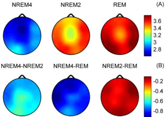
Figure 3.3 depicts the topography of average H (for the selected 90 segments) for the three vigilance states. Highest average H values emerged in the frontal region during all

Figure 3.2. Subject #16, expanded hypnogram, H and D courses corresponding to the interval denoted by the vertical black lines in Fig. 3A. (A) Hypnogram prepared according to the Rechtschaffen and Kales standard [15] using 20 s long epochs. (B) Moving average of the estimated H values for channels Fp2, Cz and O2 using a=45. (C) Moving average of the estimated D values for channels Fp2, Cz and O2 using

a=45.

Figure 3.3. (A) Subject #16, topographic maps of H averages (for the 90 selected segments of 20 s length) for sleep stages NREM4, NREM2 and REM. (B) Topographic maps for differences of the H averages between sleep stages.

(29)

vigilance states, while the minimum was found during REM in the central zone. A HNREM4 > HNREM2 > HREM trend could be observed across the whole head surface. Post- hoc tests revealed significant differences between stages NREM4 and NREM2 as well as between NREM4 and REM in all channels ( p<0.0001). Comparison of NREM2 and REM stages reached significancy at the following recording sites only: Fp1, Fp2, F3, Fz, F4, C3, Cz, C4 and P3 (p<0.0001); T3 (p<0.001); T5 (p<0.01). Difference between NREM4 and REM as well as between NREM2 and REM reached maxima in Cz electrode (Figure 3.3B).

Measure D, as expected based on the inverse course of H and D, showed an opposite trend between sleep stages: DREM > DNREM2 > DNREM4 (Figure 3.4A). During all sleep stages minima of D could be found in the fronto-central region. The central difference peak that was present for H (Figure 3.3B) disappeared in the D difference maps (Figure 3.4B). Multiple comparisons revealed significant D differences ( p<0.0001) for all sleep stage pairs in all channels.

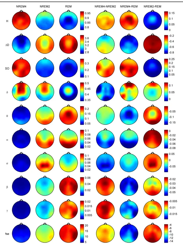
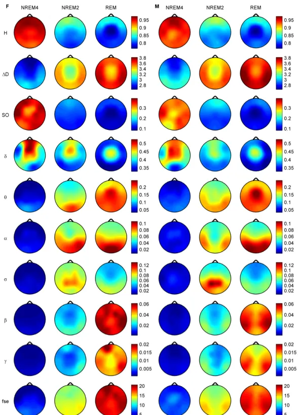
Topographic distributions of group-level medians for the three sleep stages as well as their differences are shown in Figure 3.5. Results obtained for the fractal measures were in agreement with those obtained at the individual level. Namely, highest H values emerged frontally during all sleep stages, while the minimum was found during REM in the central zone. A HNREM4 > HNREM2 > HREM trend was present across the whole head surface. Measure D, showed an opposite trend: DREM > DNREM2 > DNREM4. Minima of D could be found in the fronto-central region during all sleep stages, while higher values were observed in the posterior circumferential channels. Salient H difference peaks that occurred for sleep stage pairs NREM4-REM and NREM2-REM could not be

Figure 3.4. (A) Subject #8, topographic maps of D averages (for the 90 selected segments of 20s length) for sleep stages NREM4, NREM2 and REM. (B) Topographic maps for differences of the D averages between sleep stages.

(30)

observed in the case of D. Power spectral measures also exhibited expected topography.

Relative band powers of slow activities (SO and bands) were higher for NREM4 than NREM2 as well as for NREM2 than REM. Generally, P_SOr showed a more even topographic distribution when compared to P_δ_r in all sleep stages. Across all sleep stages

Figure 3.5. Topographic distribution of group-level medians (medians of individual medians) for the analyzed sleep stages and differences of these medians between sleep stages. Relative band powers are denoted by the labels of the corresponding frequency bands.

(31)

the minimum of P_SOroccurred at the vertex during REM sleep. Frontal regions exhibited slightly higher values of P_SOrcompared to other regions during NREM2 and REM.

During NREM4 higher P_SOr values occurred bilaterally in the fronto-temporal region and in C4, P4, O2 channels. P_δ_r exhibited higher values in the fronto-central channels during NREM4 and NREM2 and in the central region during REM sleep. Generally, faster activities (above 4 Hz) showed an opposite trend with lower relative band power values for deeper sleep stages. During NREM4 relatively even topographic distributions were found for faster activities. During NREM2 higher values appeared in the posterior region, showing maxima in the parietal channels for P_σ_r. REM sleep revealed a more diverse topography of faster activities. Maximum of theta activity was found centrally. Highest values in the and bands occurred in posterior channels. Finally, relative power of and frequency bands peaked in temporal channels. Spectral edge frequency showed lower values for deeper sleep stages as it was conjectured from Eq. (2.14). Slightly higher values of fse were present in posterior channels during NREM4 and NREM2, while during REM higher values were located in temporal channels.

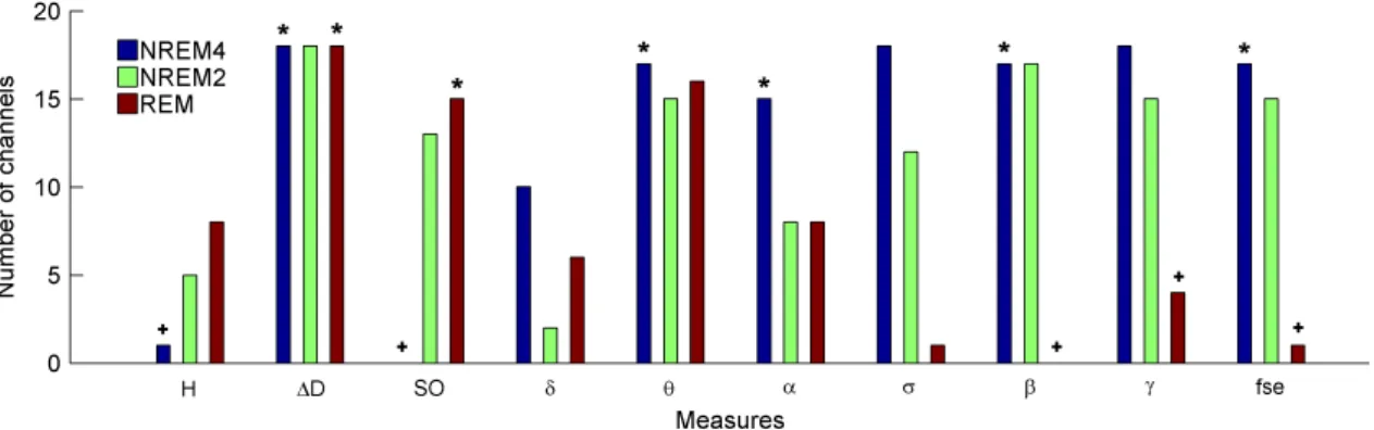
Comparing sleep stages using one-way Kruskal-Wallis ANOVA revealed highly significant (p<0.00001) differences for all measures in all channels except for the relative power of the band (Table 3.I). The level of significance for P_δ_r varied across channels between p<0.01 and p<0.00001. Pair-wise comparison of sleep stages using the rank post-hoc test resulted in most significant differences between sleep stages NREM4 and REM for all measures and channels with the exception of P_σ_r. This latter measure exhibited highest significance values between NREM4 and NREM2 in fronto- centro-parietal channels (F3, Fz, F4, C3, Cz, C4, P3 and P4). In general, least or non- significant differences were observed between sleep stages NREM2 and REM.

Comparison between NREM4 and NREM2 revealed significant values for all measures with the exception of the relative band power which reached significancy in F3, C3, P3 and P4 channels only.

3.3.1.1.Interhemispheric comparisons

As expected, Wilcoxon matched pairs test revealed (Table 3.II) more significant differences for the non-symmetric Fz-Cz channel pair as compared with the other symmetric channel pairs. Out of the 30 cases (10 measures × 3 stages) the Fz-Cz channel

SELF-ORGANIZED CRITICALITY OF THE BRAIN: FRACTAL ANALYSIS OF THE HUMAN SLEEP EEG