Evolutionary Dynamics of Cooperation in a Population with Probabilistic Corrupt Enforcers and Violators
Linjie Liu
School of Mathematical Sciences, University of Electronic Science and Technology of China, Chengdu 611731, China
Xiaojie Chen
School of Mathematical Sciences, University of Electronic Science and Technology of China, Chengdu 611731, China
xiaojiechen@uestc.edu.cn
Attila Szolnoki
Institute of Technical Physics and Materials Science, Centre for Energy Research, Hungarian Academy of Sciences, P.O. Box 49, H-1525 Budapest, Hungary
szolnoki.attila@energia.mta.hu
Abstract
Pro-social punishment is a key driver of harmonious and stable society. How- ever, this institution is vulnerable to corruption since law-violators can avoid sanctioning by paying bribes to corrupt law-enforcers. Consequently, to un- derstand how altruistic behavior survives in a corrupt environment is an open question. To reveal potential explanations here we introduce corrupt enforcers and violators into the public goods game with pool punishment, and assume that punishers, as corrupt enforcers, may select defectors probabilistically to take a bribe from, and meanwhile defectors, as corrupt violators, may select punishers stochastically to be corrupted. By means of mathematical analysis, we aim to study the necessary conditions for the evolution of cooperation in such corrupt environment. We find that cooperation can be maintained in the population in two distinct ways. First, cooperators, defectors, and punishers can coexist by all keeping a steady fraction of the population. Second, these three strate- gies can form a cyclic dominance that resembles a rock-scissors-paper cycle or a heteroclinic cycle. We theoretically identify conditions when the competing strategies coexist in a stationary way or they dominate each other in a cyclic way. These predictions are confirmed numerically.
1. Introduction
Understanding the emergence and persistence of altruistic cooperative be-
havior among selfish individuals has long been an enormous challenge.1, 2, 3, 4, 5, 6, 7, 8, 9, 10, 11, 12, 13, 14, 15
This conundrum is generally studied by using evolutionary game theory as a powerful theoretical framework.17, 18, 19, 16, 20, 21, 22 Particularly, public goods game (PGG), as a standard metaphor of the mentioned social dilemma, has at- tracted a lot of attention from broad range of research disciplines.23, 24, 25, 26, 27, 28, 29, 30, 31
In the PGG, individuals decide whether to contribute to the common pool or not, and the accumulated and enhanced contribution are distributed to group members equally. Thus defectors who contribute nothing will obtain a higher payoff, no matter what other players do. If left controlled, each individual prefers to defect in the game leading to the collapse of cooperation.32
In order to solve the problem of cooperation in the game, an intensive re-
search efforts have been carried out during the past few decades.34, 35, 36, 33, 37, 39, 38, 40, 41, 42, 43
One prominently discussed solution is the employ of punishment, that is, punish- ing uncooperative individuals by lowering their income.46, 49, 47, 50, 51, 52, 48, 44, 45, 53
In particular, two different ways of punishment are studied, namely, peer pun- ishment and pool punishment. The former refers to that group individuals can impose fines on the violators directly and its additional cost.54, 46, 55 The lat- ter means that players can decide whether to contribute to a punishment pool before contributing to the common pool of the basic game and sanctioning de- fection is organized centrally.44, 57, 56 This way of punishment is widespread and generally preferred in modern human societies.57, 56
While punishment can solve the original dilemma of cooperation, but the effectiveness of punishment in promoting cooperation has been challenged by recent theoretical research showing that the existence of corruption where de- fectors bribe corrupt officials to avoid punishment can destroy the positive consequence of costly punishment in cooperation.58, 59, 61, 60, 62 For example, Muthukrishna et al.60 experimentally showed that the possibility of corruption can cause a significant fall in public good provisioning and make empowering leaders decrease cooperative contributions.
It is worth mentioning that in most of the studies involving corruption, it is always assumed that defectors bribe corrupt enforcers and meanwhile enforcers who are involved with corruption take the bribes permanently. Indeed this as- sumption is not always justified in realistic situations where officials who are involved in corruption do not accept all the offered bribes and meanwhile civil- ians who violate the rules are not always going to offer a bribe to the officials.
In other words, corrupt officials and defective civilians may act stochastically and offer or take bribe occasionally.
Motivated by the above mentioned observations in this work we thus in- troduce corrupt enforcers and violators into the public goods game with pool punishment, and we assume that defectors bribe enforcers probabilistically to avoid punishment and meanwhile pool punishers accept a bribe from defectors also stochastically. By applying the replicator equation approach we assume infinite population where the evolutionary game dynamics is used. Our theoret- ical analysis reveals, which is also confirmed by numerical calculations, that the cooperative behavior can be maintained in the population in two different ways.
First, cooperators, defectors, and punishers can coexist where the portions of all strategies are stable in time. Alternatively, the three strategies can dominate
each other in a cyclic way similarly to the well known rock-scissors-paper cycel or a heteroclinic cycle.
2. Model and method
2.1. Public goods game
We consider the PGG played in an infinite well-mixed population. At each time step, N individuals are randomly chosen to form a group to participate in the PGG. Each individual can choose to cooperate or defect. Cooperators (C) contribute to the common pool at a cost c, while defectors (D) contribute nothing. The sum of contributions is multiplied by a factorr(1< r < N) and then the enhanced amount is divided equally among all group members.
We then introduce a third strategist, pool punishers (P), who contributeG to the punishment pool before contributing c to the common pool. They are responsible for monitoring the entire population and punishing those individu- als who are unwilling to contribute to the common pool. Alternatively, some defectors might be tempted to bribe the enforcers, so as to enable them to avoid punishment. In the same way, some enforcers can choose to accept bribes and do not punish the bribers. Here we assume that punishers decide to accept the bribebfrom corrupt defectors with probabilityp. With 1−pprobability they do not accept any bribes and punish defectors in the group. On the other hand, we assume that defector will pay the costhto bribe the corrupt punishers with probabilityq, while with 1−qprobability they are unwilling to do this. Thus, a defector who does not bribe will receive a fineB(B≥h) from every punisher no matter whether he/she is willing to accept bribe.
As a result, the payoffs of cooperators, defectors, and punishers from one PGG can be respectively written as
πC = rc(NC+NP+ 1)
N −c, (1)
πD = rc(NC+NP)
N −(1−pq)BNP−pqNPh, (2) πP = rc(NC+NP+ 1)
N −c−G+pqNDb, (3)
where NC, ND, and NP represent the number of cooperators, defectors, and pool punishers among the otherN−1 group members, respectively, and [1− p+p(1−q)]B denotes the expected fine from each punisher.
2.2. Replicator equation
We apply replicator equations to study the evolutionary dynamics of strate- gies in our model.63, 64, 65 We denote byx, y,andzthe frequencies ofC, D, and P, respectively. Thus, x, y, z≥0 and x+y+z= 1. The replicator equations are written as
{x˙ =x(PC−P¯), (4)
˙
y =y(PD−P¯), (5)
˙
z =z(PP−P¯),
(6)where PC, PD, and PP denote the expected payoffs of C, D, and P, re- spectively, and ¯P = xPC+yPD+zPP gives the average payoff of the entire population. Accordingly, the expected payoffs of the above three strategies can be written as
Pi=
N−1
X
NC=0
N−NC−1
X
ND=0
N−1NCN−NC−1NDxNCyNDzN−NC−ND−1πi, (7) wherei=C, D,or P.
In the next section, we examine the evolutionary dynamics for the men- tioned three strategies. Particulary, we analysize the distribution and stability of equilibrium points in the following section.
3. Theoretical analysis
3.1. Equilibrium points
We consider the replicator dynamics for cooperators (C), defectors (D), and pool punishers (P), with the frequenciesx, y, andz, respectively. We can get the expected payoffs of these three strategies by simplifying the formula presented in Eq. (7) as follows
PC = rc
N(N−1)(x+z) +rc
N −c, (8)
PD = rc
N(N−1)(x+z)−(1−pq)B(N−1)z−pq(N−1)zh, (9) PP = rc
N(N−1)(x+z) +rc
N −c−G+pq(N−1)yb, (10) where (N−1)(x+z) denotes the expected numbers of contributors among the N−1 co-players, and B(N −1)z gives the expected fine on a defector. The detailed analysis of the equilibrium point is shown in theorem 3.1.
The system described by (4) has at most five equilibria (x, y, z) = (1,0,0),(0,1,0),(0,0,1),(0,1−
α, α), and (1−β−µ, µ, β). Here we introduce the abbreviationα= rc/N−c−G+pq(N−1)b (B+b−h)(N−1)pq−B(N−1), β= (1−pq)B(Nc−rc/N−1)+pqh(N−1), andµ= pq(NG−1)b . It is easy to obtain the three
vertex fixed points of the above system, namely, (0,0,1),(1,0,0), and (0,1,0).
In the following, we analyze the boundary and interior equilibria of the system in detail.
We first investigate the interior equilibrium points in the simplexS3. Solving PC=PDresults inz=β. Similarly, by solvingPC =PP, we havey=µ. Thus, there is an interior equilibrium point (1−β−µ, µ, β) whenµ <1,β <1, and 1−β−µ >0.
Then we investigate the fixed points on each edge of the simplexS3. On the edgeC−Dwe havez= 0, resulting in ˙y=y(1−y)(PD−PC) =y(1−y)(c−rcN)>
0. As a result, the systems evolves fromC towardsD state.
On the C−P edge we have y = 0, resulting in ˙x=x(1−x)(PC−PP) = x(1−x)G >0. Thus the direction of the dynamics goes fromP towardCstate.
On theD−P edge we havey+z= 1, and the replicator system changes to
˙
z=z(1−z)(PP−PD). SolvingPP =PD results inz=α. Thus there exists a boundary equilibrium point (0,1−α, α) when 0< α <1.
3.2. Stability analysis of equilibria Here we set that
{f(x, y) = x[(1−x)(PC−PP)−y(PD−PP)], (11) g(x, y) = y[(1−y)(PD−PP)−x(PC−PP)].
(12)Then the Jacobian matrix of the system is J =∂f(x, y)
∂x
∂f(x, y)
∂y
∂g(x, y)
∂x
∂g(x, y)
∂y , (13)
where ∂f(x, y)
∂x = [(1−x)(PC−PP)−y(PD−PP)] +x[−(PC−PP) (14) +(1−x)∂x∂ (PC−PP)−y∂x∂ (PD−PP)], (15)
∂f(x, y)
∂y =x[(1−x)∂y∂ (PC−PP)−(PD−PP)−y∂y∂ (PD−PP)], (16)
∂g(x, y)
∂x =y[(1−y)∂x∂ (PD−PP)−(PC−PP)−x∂x∂ (PC−PP)], (17)
∂g(x, y)
∂y = [(1−y)(PD−PP)−x(PC−PP)] +y[−(PD−PP) (18) +(1−y)∂y∂ (PD−PP)−x∂y∂ (PC−PP)].
(19)
In the following, we study the stabilities of equilibria based on whether the system has an interior equilibrium point.
3.2.1. The system (4) has an interior equilibrium point
When β < 1, µ < 1, and β+µ < 1, there exists an interior fixed point, namely, (x, y, z) = (1−β−µ, µ, β). In the following we discuss the stability of this fix point.
When (1−pq)B+pqh−pqb <0, the existing interior fixed point is stable.
(1) For 0 < α < 1, there is a boundary equilibrium point with z = αon theD−P edge. Thus the system has five fixed points in the parameter space, namely, (0,0,1),(1,0,0),(0,1,0),(0,1−α, α), and (1−β−µ, µ, β).
For (x, y, z) = (0,0,1), the Jacobian is
J =G00−(1−pq)B(N−1)−pq(N−1)h−rc
N +c+G, (20)
thus the fixed equilibrium is unstable sinceG >0.
For (x, y, z) = (1,0,0), the Jacobian is J =−G−(c+G−rc
N)0c−rc
N, (21)
thus the fixed equilibrium is unstable sincer < N. For (x, y, z) = (0,1,0), the Jacobian is
J= rc
N −c0−(G−pq(N−1)b)rc
N −c−G+pq(N−1)b, (22) thus the fixed equilibrium is a saddle point and unstable since rcN −c−G+ pq(N−1)b >0.
For (x, y, z) = (0,1−α, α), the Jacobian is
J =a110a21a22, (23)
wherea11=G−pq(N−1)yb, a21=y(1−y)[pq(N−1)h+ (1−pq)(N−1)B]− y[G−pq(N−1)yb], anda22=y(1−y)(N−1)[(1−pq)B+pqh−pqb], thus the fixed equilibrium is unstable sinceG−pq(N−1)yb >0.
For (x, y, z) = (1−β−µ, µ, β), we define the equilibrium point as (x∗, y∗, z∗) hereafter, thus the elements in the Jacobian matrix are written as
∂f
∂x(x∗, y∗) = x∗[(1−x∗)∂
∂x(PC−PP)−y∗ ∂
∂x(PD−PP)], (24)
∂f
∂y(x∗, y∗) = x∗[(1−x∗)∂
∂y(PC−PP)−y∗ ∂
∂y(PD−PP)], (25)
∂g
∂x(x∗, y∗) = y∗[(1−y∗) ∂
∂x(PD−PP)−x∗ ∂
∂x(PC−PP)], (26)
∂g
∂y(x∗, y∗) = y∗[(1−y∗) ∂
∂y(PD−PP)−x∗ ∂
∂y(PC−PP)], (27)where
∂
∂x(PC−PP) = 0, (28)
∂
∂y(PC−PP) =−pq(N−1)b, (29)
∂
∂x(PD−PP) = (N−1)[pqh+ (1−pq)B], (30)
∂
∂y(PD−PP) = (N−1)[pqh+ (1−pq)B−pqb].
(31)Then we define thatp= ∂f∂x(x∗, y∗)∂g∂y(x∗, y∗)−∂f∂y(x∗, y∗)∂x∂g(x∗, y∗) and q= ∂f∂x(x∗, y∗) +∂g∂y(x∗, y∗). Thus we have
p = ∂f
∂x(x∗, y∗)∂g
∂y(x∗, y∗)−∂f
∂y(x∗, y∗)∂g
∂x(x∗, y∗)
= x∗y∗(1−x∗−y∗)[ ∂
∂x(PC−PP)∂
∂y(PD−PP)
− ∂
∂y(PC−PP) ∂
∂x(PD−PP)]
= x∗y∗(1−x∗−y∗)(N−1)2pqb[pqh+ (1−pq)B]
> 0, (32)
and
q = ∂f
∂x(x∗, y∗) +∂g
∂y(x∗, y∗)
= x∗(1−x∗) ∂
∂x(PC−PP) +y∗(1−y∗)∂
∂y(PD−PP)
− x∗y∗[ ∂
∂x(PD−PP) + ∂
∂y(PC−PP)]
= (N−1)[(1−pq)B+pqh−pqb]y∗(1−y∗−x∗). (33) Thus in the case of (1−pq)B+pqh−pqb < 0, the interior fixed point is stable.
(2) Forα≤0 orα≥1, the boundary equilibrium point of the D−P edge does not exist. Thus the system has four fixed points in the parameter space.
The stability of (0,0,1),(1,0,0),and (1−β−µ, µ, β) will not change, compared with the case of 0< α <1. Ifα≥1, the fixed point (0,1,0) is unstable since the largest eigenvalue ofJ(0,1,0) is positive. Ifα <0, the fixed point (0,1,0) is stable. Particularly, forα= 0 we can prove that this fixed point is stable by using the center manifold theorem66, 67(see Theorem.3.2.1).
When rcN −c−G+pq(N−1)b= 0, the fixed point (0,1,0) is stable.
Because ofy= 1−x−z, the dynamic equations (11) become
{x˙ =x[(1−x)(PC−PD)−z(PP−PD)], (34)
˙
z =z[(1−z)(PP−PD)−x(PC−PD)], (35)where
PC−PD = rc
N −c+ (1−pq)B(N−1)z+ (N−1)pqzh, (36) PP −PD = rc
N −c−G+pq(N−1)(1−x−z)b
+ (1−pq)B(N−1)z+pq(N−1)zh. (37) We know that (x, z) = (0,0) is an equilibrium point of system (34). Conse- quently the Jacobian is
A=rc
N −c00rc
N −c−G+pq(N−1)b. (38) When rcN −c−G+pq(N−1)b= 0, the eigenvalues of the Jacobian for the fixed point (x, z) = (0,0) are 0 and rcN −c. In this condition, we study the stability
of the equilibrium point by further using the center manifold theorem.67 To do that, we construct a matrixM, whose column elements are the eigenvectors of the matrixA, given as
M = 0110. (39)
LetT =M−1, then we have
T AT−1= 000rc
N −c. (40)
Using variable substitution, we have
vu=T xz= 0110xz=zx. (41)
Therefore, the system (3.2.1) can be rewritten as
{v˙ =v(1−v)[rcN −c−G+pq(N−1)(1−u−v)b+ (1−pq)B(N−1)v +pq(N−1)vh]−vu[rcN −c+ (1−pq)B(N−1)v+ (N−1)pqvh], (42)
˙
u =u(1−u)[rcN −c+ (1−pq)B(N−1)v+ (N−1)pqvh]−vu[rcN −c
−G+pq(N−1)(1−u−v)b+ (1−pq)B(N−1)v+pq(N−1)vh].
(43)Using the center manifold theorem,66, 67 we have thatv =e(u) is a center manifold for the above system. Then the dynamics on the center manifold, namely, the dynamics of
˙
u = u(1−u)[rc
N −c+ (1−pq)B(N−1)e(u) + (N−1)pqe(u)h]
− e(u)u[rc
N −c−G+pq(N−1)(1−u−e(u))b+ (1−pq)B(N−1)e(u)
+ pq(N−1)e(u)h], (44)
determine the dynamics near the equilibrium point. Assuming that e(u) = O(u2), thus the system (44) can be expressed as
˙
u=u(1−u)(rc
N −c) +O(|u|3). (45)
By introducingm(u) =u(1−u)(rcN−c), we havem0(u) = (1−2u)(rcN−c). Since m0(0)<0, thus we obtain that u= 0 is asymptotically stable. Therefore, we can conclude that the fixed point (u, e(u)) = (0,0) is also stable for the reduced system (34). Accordingly, the fixed point (0,1,0) is stable in the equation system (4).
Next we study the case when (1−pq)B+pqh−pqb = 0. Here the eigen- values of the Jacobian matrix for the interior equilibrium point are pure imag- inary. Besides, the boundary equilibrium point of the D−P edge does not exist. Hence the system has four fixed points in the parameter space, namely, (0,0,1),(1,0,0),(0,1,0), and (1−β−µ, µ, β). The three vertexes are unstable since the the largest eigenvalues of the Jacobi of these three fixed points are all positive.
When (1−pq)B+pqh−pqb= 0, the interior fixed point is a center surround- ing by periodic closed orbits. We introduce a new variable ε = x+yx , which represents the fraction of cooperators among individuals who do not contribute to the punishment pool. This yields
˙
ε= xy
(x+y)2(PC−PD) =−ε(1−ε)(PD−PC). (46) On the other hand, ˙z=z(PP −P), where¯
P¯ = xPC+yPD+zPP
= x(PC−PD) + (1−z)(PD−PP) +PP. (47) Thus we have
˙
z=z[x(PD−PC)−(1−z)(PD−PP)]. (48) Accordingly the equation system becomes
{ε˙ =ε(1−ε)[rcN −c+ (1−pq)B(N−1)z+ (N−1)pqzh], (49)
˙
z =z(1−z){(1−ε)[rcN −c+pq(N−1)(1−z)b +(1−pq)B(N−1)z+pq(N−1)zh]−G}.
(50)The separability of the factors allows us to write dz
dε = z(1−z)
rc
N −c+ (1−pq)B(N−1)z+ (N−1)pqzh
(1−ε)[rcN −c+pq(N−1)b]−G
ε(1−ε) ,
such that
Z rc
N −c+ (1−pq)B(N−1)z+ (N−1)pqzh
z(1−z) dz
=
Z (1−ε)[rcN −c+pq(N−1)b]−G
ε(1−ε) dε. (51)
The integral of the right-hand side is [rc
N −c+pq(N−1)b] log(ε)−G[log(ε)−log(1−ε)]. (52) The integral of the left-hand side is
(c−rc
N)[log(z)−log(1−z)]−[(1−pq)B(N−1)
+(N−1)pqh] log(1−z). (53) In this way, we identify the constant of motion
H(ε, z) = [rc
N −c+pq(N−1)b] log(ε)−G[log(ε)−log(1−ε)]
+ (c−rc
N)[log(z)−log(1−z)]−[(1−pq)B(N−1)
+ (N−1)pqh] log(1−z). (54)
Therefore, we have
H˙ = ∂H
∂εε˙+∂H
∂zz˙= 0. (55)
Accordingly, the system is conservative and all constant level sets of H cor- respond to closed curves. Besides, the interior fixed point is neutrally stable surrounded by those closed and periodic orbits.
Last, when (1−pq)B+pqh−pqb >0, the existing interior fixed point is unstable.
(1) For 0 < α < 1, there is a boundary equilibrium point on the D−P edge. Then the system has five fixed points in the parameter space, namely, (0,0,1),(1,0,0),(0,1,0),(0,1−α, α), and (1−β−µ, µ, β).
The fixed points (0,0,1),(1,0,0),and (0,1−α, α) are all unstable since the largest eigenvalues of the Jacobi are all positive.
For (x, y, z) = (0,1,0), the Jacobian is J= rc
N −c0−(G−pq(N−1)b)rc
N −c−G+pq(N−1)b, (56) thus this is a stable equilibrium point since rcN −c−G+pq(N−1)b <0.
(2) For α ≤ 0 or α ≥ 1, the boundary equilibrium point of the D−P edge does not exist. Thus the system has four fixed points in the mentioned parameter space. The stability of (0,0,1),(1,0,0),and (1−β−µ, µ, β) will not change, compared with the case of 0< α <1. If α≥1, the fixed point (0,1,0) is unstable since the largest eigenvalue of J(0,1,0) is positive. If α≤ 0, the fixed point (0,1,0) is stable.
WhenrcN−c−G >max{−(N−1)[(1−pq)B+pqh],−pq(N−1)b}andr < N, there is a stable heteroclinic cycle on the boundary of the simplexS3.
When rcN −c−G > max{−(N−1)[(1−pq)B +pqh],−pq(N−1)b}, and r < N, we know that the three vertex equilibrium points (C, D, and P) are all saddle nodes, and the three edges (CD, DP, and P C) are the heteroclinic trajectories. All of these guarantee the existence of the heteroclinic cycle on the boundaryS3. In the following, we will prove that the heteroclinic cycle is asymptotically stable.
Based on the above analysis, we can get the eigenvalues of the Jacobian matrix of the three vertex equilibrium points, namely, λ−P = −(N −1)[(1− pq)B +pqh]−(rcN −c−G), λ+P = G, λ−C = −G, λ+C = c− rcN, λ−D = rcN −c, andλ+D = rcN −c−G+pq(N−1)b, respectively. Then we respectively define that λP = −λ
− P
λ+P, λC = −λ
− C
λ+C, and λD = −λ
− D
λ+D, and we have λ = λPλCλD =
rc
N−c−G+(N−1)[(1−pq)B+pqh]
rc
N−c−G+pq(N−1)b . When (1−pq)B+pq(h−b)>0, we have λ > 1.
Therefore the heteroclinic cycle is asymptotically stable.68 3.2.2. There is no interior equilibrium point in the system (4)
Whenβ≥1, orµ≥1, orβ+µ≥1, the interior fixed point does not exist.
(1) For 0 < α < 1, there is a boundary equilibrium point on the D−P edge. Then the system has four fixed points in the parameter space, namely, (0,0,1),(1,0,0),(0,1,0),and (0,1−α, α).
The fixed points (0,0,1) and (1,0,0) are both unstable since the largest eigenvalues of Jacobi are both positive.
For (x, y, z) = (0,1,0), the Jacobian is J= rc
N −c0−(G−pq(N−1)b)rc
N −c−G+pq(N−1)b, (57) thus the fixed equilibrium is a saddle point and unstable when rcN −c−G+ pq(N−1)b >0, while when rcN −c−G+pq(N−1)b <0, it is stable.
For (x, y, z) = (0,1−α, α) fixed point the Jacobian is
J =a110a21a22, (58)
wherea11=G−pq(N−1)(1−α)b, a21=α(1−α)[pq(N−1)h+ (1−pq)(N− 1)B]−(1−α)[G−pq(N−1)αb], anda22=α(1−α)(N−1)[(1−pq)B+pqh− pqb], thus the fixed equilibrium is stable when pqb > max{(N−1)(1−α)G ,(1− pq)B+pqh}, and it is unstable whenpqb <max{(N−1)(1−α)G ,(1−pq)B+pqh}.
Particularly, whenpqb = max{(N−1)(1−α)G ,(1−pq)B+pqh}, we find that one eigenvalue of the Jacobian matrix at this fixed point is zero and the other one is negative. Accordingly, we study its stability by further using the center manifold theorem67as follows.
For 0< α <1, we knowpqb6= (1−pq)B+pqhand max{(N−1)yG ,(1−pq)B+ pqh} = (N−1)yG . In order to use the center manifold theorem conveniently, we takeξ=y−1 +αandη=z−α, then the equation system becomes
nξ˙ = (1 +ξ−α)
(α−ξ)[c−rcN −(1−pq)B(N−1)(α+η)
−(N−1)pqh(α+η)]−(α+η)[pq(N−1)(1 +ξ−α)b−G] ,
˙
η = (α+η)
(1−α−η)[pq(N−1)(1 +ξ−α)b−G]−(1 +ξ−α)[c
−rcN −(1−pq)B(N−1)(α+η)−(N−1)pqh(α+η)] ,
We further let M be a matrix whose columns are the eigenvectors ofJ(0,1− α, α) which can be written as M= a11−a22a21011. Then we have M−1J(0,1− α, α)M = 00
0a22. We further take [u v]T =M−1[ξ η]T, and thus we have u=ξ/θ and v=η−ξ/θwhere we used the notationθ= a11a−a22
21 . It leads to
˙
u = 1
θ(1−α+uθ)n
(α−uθ) c−rc
N −(1−pq)B(N−1)(α+u+v)
− (N−1)pqh(α+u+v)
−(α+u+v)
pq(N−1)(1 +uθ−α)b−Go .
Using the center manifold theorem, we have thatv=e(u) is a center manifold.
We assume thate(u) =O(|u|2), which yields the reduced system
˙
u = 1
θ(1−α+uθ)n
(α−uθ)(c−rc
N)−(N−1)(α+u)
(α−uθ)(1−pq)B
+ (α−uθ)pqh+pqubθo .
By introducing m(u) = θ(1−α+uθ)n
(α−uθ)(c− rcN)−(N −1)(α+ u)
(α−uθ)(1−pq)B+ (α−uθ)pqh+pqubθo
, we havem0(u) = (α−uθ)(c−
rc
N)−(N−1)(α+u)
(α−uθ)(1−pq)B+ (α−uθ)pqh+pqubθ
+ (1θ− 1θα+ u)
−θ(c− rcN)−(N −1)
(α−uθ)(1−pq)B+ (α−uθ)pqh+pqubθ
−(N − 1)(α+u)
−θ(1−pq)B−θpqh+pqbθ . By calculation, we know m0(0) =
−(1−α)n
c−rcN+(N−1)α1θ[(1−pq)B+pqh]+α(N−1)[pqb−(1−pq)B−pqh]o
<0, thus we obtain thatu= 0 is asymptotically stable. Therefore we also know that the fixed point (u, e(u)) = (0,0) is stable for the reduced system. Accordingly, the fixed point (0,1−α, α) is stable.
(2) Forα≤0 orα≥1, the boundary equilibrium point of the D−P edge does not exist. Then the system has only three fixed points in the parameter space, namely, (0,0,1),(1,0,0),and (0,1,0).
The fixed point (0,0,1) and (1,0,0) are both unstable since the largest eigen- values of corresponding Jacobi are both positive. If rcN −c−G+pq(N−1)b≤0, the fixed point (0,1,0) is stable, while it is a saddle point and becomes unstable when rcN −c−G+pq(N−1)b >0.
4. Numerical examples
We now provide some numerical examples to confirm the above theoretical analysis. We use the simplexS3={(x, y, z) :x, y, z≥0, x+y+z= 1}to depict the state space of above three strategies. Accordingly, the three homogeneous states C (x = 1), D (y = 1), and P (z = 1) correspond to three corners of the simplexS3. All of these are equilibrium points of the system (4). We first present numerical cases when the system (4) has an interior equilibrium point.
Whenβ <1, µ < 1, andβ+µ <1, there is an interior fixed point. From the theoretical analysis we know that its stability is determined by the relationship between the expected loss of defectors [(1−pq)B+pqh] and the expected bribe amount received by punishers (pqb).
4.1. Stable interior equilibrium point
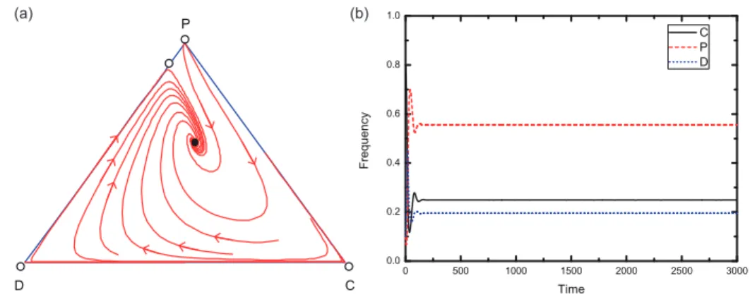
In the following we present a numerical example to confirm that the system can have a stable interior equilibrium point. As shown in Fig. 1(a), we see that there exist five equilibria in the simplexS3. The existing interior equilibrium point is stable and all interior orbits converge to this point, irrespective of the initial conditions. Besides, an interior equilibrium point between all defectors and all punishers enters the edgeD−P, which is unstable. Furthermore, the direction of the evolution on theC−P edge is fromP toC, and fromC toD on theC−D edge. Figure 1(b) depicts the time evolution of the frequencies of cooperators, defectors, and punishers. We can see that all mentioned strategies
can coexist when the system reaches the steady state. Furthermore, the fraction of punishers is the highest, and the fraction of defectors is the lowest.
It is worth noting that all these results above are consistent with the the- oretical results. In particular, when (1−pq)B+pqh−pqb < 0, the interior equilibrium point is stable. And the boundary fixed point withz=αonD−P edge can appear when 0 < α < 1. According to our theoretical analysis, we know that it is unstable sinceG−pq(N−1)(1−α)b >0 (more detailed analysis can be seen in Theorem 3.1 and in Subsection 3.2.1).
4.2. Hamiltonian system
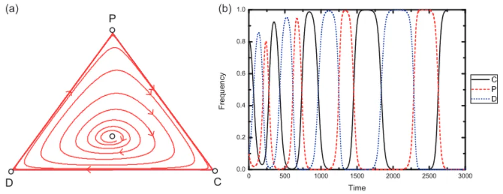
In this section we provide a numerical example to confirm that the system can become Hamiltonian. In Fig. 2(a), we see that the existing interior equilib- rium point is a center surrounded by periodic orbits and the strategy evolution display a limit cycle. No boundary fixed points can be detected on the three edges. And the direction of evolution on theD−P edge is fromD toP, from P toC on theP −C edge, and fromC to D on theC−D edge. Figure 2(b) depicts that the frequencies of these three strategies display periodic oscilla- tions in dependence of time, which is corresponding to the limit cycle shown in Fig. 2(a). All these results are in agreement with the theoretical prediction, namely, when (1−pq)B+pqh−pqb= 0, the interior fixed point is neutrally stable, and the dynamic system is Hamiltonian (see Theorem 3.2.1 of Section 3 for detailed theoretical analysis).
The cyclical evolutionary scenario can be described as follows. If most play- ers are cooperators in the group, it is better to become a defector due to the social dilemma. If defectors are prevalent, corrupt officials can get a lot of bribes from a group of defectors, and thus the number of punishers increases. If most players are punishers, the bribes from a few defectors are usually small enough to subvert cooperators dominance over punishers, and thus cooperators spread.
If the number of cooperators increases sufficiently, then the original cooperation dilemma returns. It is worth noting that cooperative behavior can still emerge even in a completely corrupt environment. As we set that p =q = 1, which means that all defectors are willing to offer a bribe to punishers, and all pun- ishers are corrupt officials. It is inspiring to see that altruistic behavior can still be maintained since the oscillations recurrent increase in cooperation.
4.3. Heteroclinic cycle
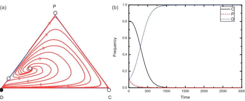
We provide a numerical example to confirm that the heteroclinic cycle can exist in our system. Figure 3(a) shows that there are four unstable fixed points in the simpleS3, and all interior curves of state space converge to the boundary of S3. Besides, the direction of the evolution on the D −P edge is from D to P, on the P −C edge is from P to C, while on the C −D edge is from C to D. Figure 3(b) depicts that the frequencies of the three strategies are oscillating and the amplitudes are gradually growing, eventu- ally forming periodic oscillations. This means that these three strategies can be cyclically dominant in the population and thus can avoid the tragedy of
the commons. Note that these numerical results are in agreement with the theoretical analysis which states that the population converges to a stable heteroclinic cycle on the boundary of S3 for (1 −pq)B +pqh−pqb > 0,
rc
N −c−G > max{−(N −1)[(1−pq)B +pqh],−pq(N −1)b}, and r < N (Theorem 3.2.1 of Section 3).
4.4. Global stability of all-D state
Next we provide a numerical example to confirm that the equation system can converge to the all-D state with global stability when the interior equilib- rium point is unstable. As shown in Fig. 4(a), there are five fixed points in the simplexS3. All interior orbits coverage to the vertexD, which is a global stable equilibrium point. In the boundary case the unstable equilibrium point on the D −P edge reappears. Besides, defectors can always do better than cooperators on theC−D edge, and punishers are always weaker than cooper- ators on the remainingC−P edge. In Fig. 4(b), we show how the frequency of the three strategies evolves in time when the initial fractions of cooperators, defectors, and punishers are 0.8, 0.1, and 0.1, respectively. Finally the fraction of defectors reaches one. This numerical behavior is in agreement with our the- oretical prediction which says that the system converges on the all-D state for
rc
N −c−G+pq(N−1)b≤0 (Subsection 3.2.1).
4.5. Boundary equilibrium point with the coexistence of defectors and punishers Finally we present a numerical example to confirm that there exists a stable boundary equilibrium point with the coexistence of defectors and punishers. In Fig. 5(a), we show that the system converges to the stable boundary equilibrium point on the D−P edge, irrespective of the initial conditions, which means that defectors and punishers can coexist permanently in the population, while cooperators disappear. Besides, the evolutionary direction on C−D edge is from C to D, while it is from P to C on the C−P edge. Figure 5(b) shows that the fraction of cooperators gradually decays to 0, even though their initial frequency is relatively high. In parallel the fraction of punishers finally reaches about 0.8, while the fraction of defectors saturates about 0.2. These numerical results validate our theoretical analysis based on which as long as the interior equilibrium does not exist, the boundary fixed point on the D −P edge is globally stable (Subsection 3.2.2).
5. Conclusions
In this paper, we have introduced probabilistic corrupt enforcers and viola- tors into the public goods game and investigated their consequence on the evo- lution of cooperation and punishment in infinite well-mixed populations. As a result, we have observed basically two different evolutionary scenarios. Namely, the competing strategies either coexist by forming stable time-dependent frac- tions or they dominate each other in a rock-scissors-paper game like manner.
But for both cases the cooperative behavior can be well preserved. We have fur- ther identified the conditions in which the two dynamic behaviors can appear.
We find that when the expected loss is less than the related bribe amount, a stable coexistence state among these three strategists can appear. In the alterna- tive case, when these two quantity values are identical, the replicator dynamical system can be reduced to a Hamiltonian system. Here a center surrounded by closed orbits appears in the interior of the simplexS3, which means that these three strategies are mutually restrained and exhibit periodic oscillations. When the expected loss is larger than the expected bribe amount, the interior fixed point is unstable, and two different evolutionary dynamic behaviors can emerge, namely, stable heteroclinic cycle and global attractorD. The former can guar- antee that cooperators, defectors, and punishers are cyclically dominant in the population, while the latter will lead to the tragedy of commons.
The key feature of our model is that corruption may emerge stochastically, either from the side of violators or from corrupt enforcers. This realistic as- sumption can be modeled in infinite well-mixed population by using replicator equations. The study of such highly nonlinear equation systems is really chal- lenging,69, 37 but we could manage a comprehensive and systematic theoretical analysis. We could identify all equilibrium points and characterize their stabil- ity by appropriately linearizing the equation system. In particular, we cannot determine the stability of an equilibrium point based only on the eigenvalues of the Jacobian. Instead, we investigate its stability by utilizing the center mani- fold theorem.66, 67 Furthermore, we not only prove that the system can exhibit the central limit cycle, but also theoretically confirm the existence and stability of heteroclinic cycle.
Recently, Huang et al.62 investigated the effect of corruption on the evolution of cooperation and punishment in a hierarchical society which is divided into civilians and cops. Our present work, however, focuses on the evolutionary dy- namics of cooperation, defection, and punishment in an integrated society when corruption is possible. Importantly, we consider that defectors probabilistically bribe enforcers to avoid punishment and meanwhile pool punishers probabilisti- cally accept a bribe from defectors, which can reflect a realistic behavior manner of individuals in human societies. This behavior was studied in a population where individuals play the public goods game with pool punishment,70and thus provide an alternative, but reasonable route to study the effects of corruption on collective actions of cooperation. Rather unexpectedly, the introduction of corruption can stabilize cooperation, and more interesting dynamic behaviors can be derived which may provide some implications for designing sanctioning strategies to support the evolution of cooperation.
We point out that although cooperative behavior can occur in a corrupt en- vironment, the long-term existence of corruption will weaken social fairness and justice. We should stress that our present model does not explicitly consider a strategy chance of an anti-corruption control which could be an additional source of cooperation support. Such kind of extension could be the scope of fu- ture research. On the other hand, however, although powerful anti-corruption monitoring and sanctioning have been used to resolve the corruption problem,
the effects of such measures are either transient or uncertain.58, 59, 60, 71, 62 For example, Muthukrishna et al.60 found that anti-corruption strategies are effec- tive under some conditions, but can further decrease public good provisioning when leaders are weak and the economic potential is poor even if these strate- gies are powerful. Consequently, the task how to design efficient anti-corruption strategies for resisting the occurrence of corruption remains an open question.
Acknowledgment
This research was supported by the National Natural Science Foundation of China (Grant No. 61503062) and by the Hungarian National Research Fund (Grant K-120785).
[1] W. D. Hamilton, The evolution of altruistic behavior,Am. Nat.97(1963) 354-356.
[2] E. Fehr and U. Fischbacher, The nature of human altruism, Nature 425 (2003) 785–791.
[3] A. Szolnoki and G. Szab´o, Cooperation enhanced by inhomogeneous activ- ity of teaching for evolutionary Prisoner’s Dilemma games, EPL77(2006) 30004.
[4] F. C. Santos, M. D. Santos, and J. M. Pacheco, Social diversity promotes the emergence of cooperation in public goods games, Nature 454 (2008) 213–216.
[5] N. Bellomo, H. Berestycki, F. Brezzi, and J. Nadal, Mathematics and com- plexity in life and human sciences, Math. Models Methods Appl. Sci. 19 (2009) 1385-1389.
[6] N. Bellomo, F. Brezzi, and M. Pulvirenti, Modeling behavioral social sys- tems,Math. Models Methods Appl. Sci.27 (2016) 1–11.
[7] J. M. Allen, A. C. Skeldon, and R. B. Hoyle, Social influence preserves cooperative strategies in the conditional cooperator public goods game on a multiplex network,Phys. Rev. E98 (2018) 062305.
[8] N. Bellomo and S. Y. Ha, A quest toward a mathematical theory of the dynamics of swarms,Math. Models Methods Appl. Sci.27(2017) 745–770.
[9] M. A. Herrero and J. Soler, Cooperation, competition, organization: The dynamics of interacting living populations, Math. Models Methods Appl.
Sci. 25(2015) 2407–2415.
[10] M. Dolfin and M. Lachowicz, Modeling altruism and selfishness in welfare dynamics: The role of nonlinear interactions, Math. Models Methods Appl.
Sci. 24(2014) 2361-2381.
[11] A. Szolnoki and X. Chen, Competition and partnership between conformity and payoff-based imitations in social dilemmas, New J. Phys. 20 (2018) 093008.
[12] F. C. Santos, F. L. Pinheiro, T. Lenaerts, and J. M. Pacheco, The role of diversity in the evolution of cooperation,J. Theor. Biol.299(2012) 88–96.
[13] M.-J. Fu and H.-X. Yang, Stochastic win-stay-lose-learn promotes cooper- ation in the spatial public goods game, Int. J. Mod. Phys. C 29 (2018) 1850034.
[14] M. Perc, J. J. Jordan, D. G. Rand, and Z. Wang, S. Boccaletti, and A.
Szolnoki, Statistical physics of human cooperation,Phys. Rep.687(2017) 1–51.
[15] X. Chen and A. Szolnoki, Punishment and inspection for governing the commons in a feedback-evolving game, PLOS Comp. Biol. 14 (2018) e1006347.
[16] M. Perc and A. Szolnoki, Social diversity and promotion of cooperation in the spatial prisoner’s dilemma game, Phys. Rev. E77(2008) 011904.
[17] M. Perc and A. Szolnoki, Coevolutionary games–a mini review,BioSystems 99 (2010) 109–125.
[18] F. Fu, M. A. Nowak, and C. Hauert, Invasion and expansion of cooperators in lattice populations: Prisoner’s dilemma vs. snowdrift games, J. Theor.
Biol.266(2010) 358–366
[19] Q. Chen, T. Chen, and Y. Wang, How the expanded crowd-funding mech- anism of some southern rural areas in China affects cooperative behaviors in threshold public goods game, Chaos, Solitons and Fractals 91 (2016) 649–655.
[20] A. Szolnoki and Z. Danku, Dynamic-sensitive cooperation in the presence of multiple strategy updating rules,Physica A511(2018) 371–377.
[21] F. C. Santos, V. V. Vasconcelos, M. D. Santos, P. N. B. Neves, and J.
M. Pacheco, Evolutionary dynamics of climate change under collective-risk dilemmas,Math. Models Methods Appl. Sci.22(2012) 1140004.
[22] V. V. Vasconcelos, F. C. Santos, and J. M. Pacheco, Cooperation dynamics of polycentric climate governance, Math. Models Methods Appl. Sci. 25 (2015) 2503–2517.
[23] M. Milinski, D. Semmann, and H. J. Krambeck, Reputation helps solve the
‘tragedy of the commons’, Nature415(2002) 424.
[24] C. Hauert, S. De Monte, J. Hofbauer, and K. Sigmund, Volunteering as red queen mechanism for cooperation in public goods games, Science296 (2002) 1129–1132.
[25] F. Fu, X. Chen, L. Liu, and L. Wang, Social dilemmas in an online social network: the structure and evolution of cooperation, Phys. Lett. A 371 (2007) 58–64.
[26] C. Hilbe, L. Schmid, J. Tkadlec, K. Chatterjee, and M. A. Nowak, Indirect reciprocity with private, noisy, and incomplete information, Proc. Natl.
Acad. Sci. USA115(2018) 12241-12246.
[27] A. Szolnoki and M. Perc, Resolving social dilemmas on evolving random networks,EPL86(2009) 30007.
[28] T. Wu, F. Fu, P. Dou, and L. Wang, Social influence promotes cooperation in the public goods game,Physica A413(2014) 86–93.
[29] A. Szolnoki and X. Chen, Environmental feedback drives cooperation in spatial social dilemmas,EPL120(2017) 58001.
[30] X. Chen, Y. Zhang, T. Huang, and M. Perc, Solving the collective-risk social dilemma with risky assets in well-mixed and structured populations, Phys. Rev. E90 (2014) 052823.
[31] N. He, X. Chen, and A. Szolnoki. Central governance based on monitoring and reporting solves the collective-risk social dilemma, Appl. Math. Com- put. 347(2019) 334–341.
[32] G. Hardin, The tragedy of the commons,Science162(1968) 1243–1248.
[33] F. C. Santos, C. Francisco, and J. M. Pacheco, Risk of collective failure provides an escape from the tragedy of the commons, Proc. Natl. Acad.
Sci. USA 108(2011) 10421–10425.
[34] M. A. Nowak, Five rules for the evolution of cooperation, Science 314 (2006) 1560–1563.
[35] A. Szolnoki and X. Chen, Reciprocity-based cooperative phalanx main- tained by overconfident players, Phys. Rev. E 98(2018) 022309.
[36] F. Fu, C. Hauert, M. A. Nowak, and L. Wang, Reputation-based partner choice promotes cooperation in social networks, Phys. Rev. E 78 (2008) 026117.
[37] T. Sasaki and T. Unemi, Replicator dynamics in public goods games with reward funds,J. Theor. Biol. 287(2011) 109–114.
[38] X. Chen, A. Szolnoki, and M. Perc, Risk-driven migration and the collective-risk social dilemma, Phys. Rev. E86(2012) 036101.
[39] A. Szolnoki and M. Perc, Evolutionary advantages of adaptive rewarding, New J. Phys.14(2012) 93016.
[40] T. Sasaki, S. Uchida, and X. Chen, Voluntary rewards mediate the evolu- tion of pool punishment for maintaining public goods in large populations, Sci. Rep.5(2015) 8917.
[41] T. Sasaki, A. Br¨annstr¨om, U. Dieckmann, and K. Sigmund, The take-it- or-leave-it option allows small penalties to overcome social dilemmas,Proc.
Natl. Acad. Sci. USA109(2012) 1165–1169,
[42] Z. Pei, B. Wang, and J. Du, Effects of income redistribution on the evolu- tion of cooperation in spatial public goods games,New J. Phys. 19(2017) 013037.
[43] T. Wu, F. Fu, and L. Wang, Coevolutionary dynamics of aspiration and strategy in spatial repeated public goods games, New J. Phys. 20 (2018) 063007.
[44] A. Szolnoki, G. Szab´o, and M. Perc, Phase diagrams for the spatial public goods game with pool punishment,Phys. Rev. E83(2011) 036101.
[45] X. Chen, A. Szolnoki, and M. Perc, Probabilistic sharing solves the problem of costly punishment,New J. Phys.16(2014) 083016.
[46] B. Rockenbach and M. Milinski, The efficient interaction of indirect reci- procity and costly punishment, Nature444(2006) 718–723.
[47] T. Sasaki and S. Uchida, The evolution of cooperation by social exclusion, Proc. R. Soc. B280(2012) 20122498.
[48] A. Szolnoki and M. Perc, Effectiveness of conditional punishment for the evolution of public cooperation, J. Theor. Biol.325(2013) 34–41.
[49] X. Chen, T. Sasaki, ˚A. Br¨annstr¨om, and U. Dieckmann, First carrot, then stick: how the adaptive hybridization of incentives promotes cooperation, J. Roy. Soc. Interface 12(2014) 20140935.
[50] L. Liu, X. Chen, and A. Szolnoki, Competitions between prosocial exclu- sions and punishments in finite populations, Sci. Rep.7(2017) 46634.
[51] L. Liu, S. Wang, X. Chen, and M. Perc, Evolutionary dynamics in the pub- lic goods games with switching between punishment and exclusion,Chaos, 28 (2018) 103105.
[52] A. Szolnoki and X. Chen, Alliance formation with exclusion in the spatial public goods game, Phys. Rev. E95(2017) 052316.
[53] H. X. Yang and X. Chen, Promoting cooperation by punishing minority, Appl. Math. Comput. 316(2018) 460–466.
[54] E. Fehr and S. G¨achter, Altruistic punishment in humans, Nature, 415 (2002) 137.
[55] J. Andreoni, W. Harbaugh, and L. Vesterlund, The carrot or the stick:
Rewards, punishments, and cooperation, Am. Econ. Rev. 93 (2003) 893–
902.
[56] K. Sigmund, H. De Silva, A. Traulsen, and C. Hauert, Social learning promotes institutions for governing the commons,Nature466(2010) 861–
863.
[57] A. Traulsen, T. R¨ohl, and M. Milinski, An economic experiment reveals that humans prefer pool punishment to maintain the commons, Proc. R.
Soc. B279(2012) 3716–3721.
[58] S. Abdallah, R. Sayed, I. Rahwan, B. L. LeVeck, M. Cebrian, A. Ruther- ford, and J. H. Fowler, Corruption drives the emergence of civil society,J.
Roy. Soc. Interface11(2014) 20131044.
[59] J. H. Lee, M. Jusup, and Y. Iwasa, Games of corruption in preventing the overuse of common-pool resources, J. Theor. Biol.428(2017) 76–86.
[60] M. Muthukrishna, P. Francois, S. Pourahmadi, and J. Henrich, Corrupting cooperation and how anti-corruption strategies may backfire, Nat. Hum.
Behav.1(2017) 0138.
[61] P. Verma and S. Sengupta, Bribe and punishment: An evolutionary game- theoretic analysis of bribery,PLoS ONE10(2015) e0133441.
[62] F. Huang, X. Chen, and L. Wang, Evolution of cooperation in a hierarchical society with corruption control,J. Theor. Biol. 449(2018) 60–72.
[63] P. Schuster and K. Sigmund, Replicator dynamics, J. Theor. Biol. 100 (1983) 533–538.
[64] J. Hofbauer and K. Sigmund,Evolutionary games and population dynamics, (Cambridge University Press, 1998).
[65] Q. Wang, N. He, and X. Chen, Replicator dynamics for public goods game with resource allocation in large populations, Appl. Math. Comput. 328 (2018) 162–170.
[66] J. Carr, Applications of Center Manifold Theory, (Springer Verlag, New York, 1981)
[67] H. K. Khalil,Noninear systems, (Prentice-Hall, New Jersey, 1996)
[68] J. Park, Balancedness among competitions for biodiversity in the cyclic structured three species system,Appl. Math. Comput.320(2018) 425–436.
[69] C. Hauert, S. De Monte, J. Hofbauer, and K. Sigmund, Replicator dynamics for optional public good games, J. Theor. Biol.218(2002) 187–194.
[70] K. Sigmund, C. Hauert, A. Traulsen, and H. De Silva, Social Control and the Social Contract: The Emergence of Sanctioning Systems for Collective Action,Dyn. Games Appl.1(2011) 149–171.
[71] P. Verma, A. K. Nandi, and S. Sengupta, Bribery games on inter-dependent regular networks,Sci. Rep.7(2017) 42735.
0 500 1000 1500 2000 2500 3000 0.0
0.2 0.4 0.6 0.8 1.0
Frequency
Time
C P D P
C D
(a) (b)
Figure 1: The evolution of cooperation in an environment where corruption loss and bribe are unequal. The triangle represents the state space where the actual fractions of cooperators, defectors, and punishers are denoted ∆ ={(x, y, z) :x, y, z ≥0 andx+y+z= 1}. The filled circle represents a stable fixed point whereas open circles represent unstable fixed points.
Panel (a) depicts that a stable interior equilibrium appears in the simplexS3, which means that these three strategies coexist by maintaining a stable fraction in the population. Panel (b) depicts time series of the frequencies of three strategiesC (cooperators, black solid line),D (defectors, blue dot line), andP (pool punishers, red dash line). After an initial transient the frequencies of the three strategies eventually stabilizes in time. Initial conditions: (x, y, z) =
22
0 500 1000 1500 2000 2500 3000 0.0
0.2 0.4 0.6 0.8 1.0
Frequency
Time
C P D P
C D
(a) (b)
Figure 2: The evolution of cooperation in a corrupt environment when loss and bribe are equal.
Panel (a) depicts that there is an interior fixed point which is surrounded by periodic orbits in the simplex. Panel (b) depicts a representative behavior when strategies are oscillating amongC,D, andP states. Initial conditions: (x, y, z) = (0.8,0.1,0.1). Parameters: N= 5, r= 3,c= 1,G= 0.5,B= 0.5,h= 0.4, b= 0.4, q= 1, andp= 1.
D C
P
0 500 1000 1500 2000 2500 3000
0.0 0.2 0.4 0.6 0.8 1.0
Frequency
Time
C P D
(a) (b)
Figure 3: The evolution of cooperation in a corrupt environment when bribe acceptance is more intensive. Panel (a) depicts that the interior equilibrium point turns into a repeller, and the interior curves of simplex S3 coverage to the boundary of S3. Panel (b) depicts that the frequencies of these three strategies display growing periodic oscillations. Initial conditions: (x, y, z) = (0.8,0.1,0.1).Parameters: N = 5,r= 3,c= 1,G= 0.5,B= 0.5,
P
D C
0 500 1000 1500 2000 2500 3000
0.0 0.2 0.4 0.6 0.8 1.0
Frequency
Time
C P D
(a) (b)
Figure 4: The evolution of cooperation in an environment when corruption loss exceeds the expected bribe. Panel (a) depicts that the defection has an evolutionary advantage over the other two strategies, and ultimately occupies the entire population. Panel (b) illustrates the time evolution how strategyDprevails in the whole population. Initial conditions: (x, y, z) = (0.8,0.1,0.1).Parameters: N= 5,r= 3,c= 1,G= 0.5,B= 0.5,h= 0.4, b= 0.2, q= 1, and
0 2000 4000 6000 8000 10000 0.0
0.2 0.4 0.6 0.8 1.0
Frequency
Time
C P D
P
C D
(a) (b)
Figure 5: The evolution of cooperation in a corrupt environment when bribe is overvalued by acceptors. Panel (a) depicts that there exists a stable boundary equilibrium point onP−D edge, and all trajectories starting from different initial conditions terminate onto this point.
Panel (b) illustrates thatD and P can form a stable coexistence in the population. Initial conditions: (x, y, z) = (0.8,0.1,0.1).Parameters: N = 5,r= 3,c= 1,G= 0.5,B= 0.5,