correlation
Szil´ard Szalay
Strongly Correlated Systems “Lend¨ulet” Research Group,
Wigner Research Centre for Physics of the Hungarian Academy of Sciences, 29-33, Konkoly-Thege Mikl´os ´ut, Budapest, H-1121, Hungary
E-mail: szalay.szilard@wigner.mta.hu
Abstract. In multipartite entanglement theory, the partial separability properties have an elegant, yet complicated structure, which becomes simpler in the case when multipartite correlations are considered. In this work, we elaborate this, by giving necessary and sufficient conditions for the existence and uniqueness of the class of a given class-label, by the use of which we work out the structure of the classification for some important particular cases, namely, for the finest classification, for the classification based onk-partitionability andk-producibility, and for the classification based on the atoms of the correlation properties.
PACS numbers: 03.65.Fd, 03.65.Ud, 03.67.Mn
1. Introduction
In quantum systems, nonclassical forms of correlations arise, which, although being simple consequences of the Hilbert space structure of quantum mechanics, represent a longstanding challenge for the classically thinking mind. Pure states of classical systems are always uncorrelated; correlations in pure states are of quantum origin, this is what we call entanglement [1, 2]. The correlation inmixed states of classical systems can be induced by classical communication; correlations in mixed states which are not of this kind are of quantum origin, this is what we call entanglement [3, 2].
Bipartitesystems can either be uncorrelated or correlated, and either be separable or entangled, while for multipartite systems, the partial separability properties have a complicated, yet elegant structure [4, 5, 6, 7, 8, 9, 10, 11]. Considering the partial correlation properties of multipartite systems [11], the structure of the classification [10] becomes simpler. In the present work, we elaborate this, by giving necessary and sufficient conditions for the existence and uniqueness of the class of a given class-label, by the use of which we elaborate the structure of the classification in some important particular cases.
Our work is motivated by that quantum correlation and entanglement are of central importance in many fields of research in quantum physics nowadays, first of all in quantum information theory [12, 13, 14] and in strongly correlated manybody systems [15,16,17]. Especially in the latter case, correlation might be more important than entanglement, since in physical properties of manybody systems, the entire correlation is what matters, not only its entanglement part. (The two coincide only for pure states, so almost never inside subsystems.) Fortunately, this also meets
arXiv:1806.04392v2 [quant-ph] 15 Nov 2018
the claim of practice, since the measures of multipartite correlations are feasible to evaluate [10, 11], while this is not the case for the measures of multipartite entanglement [18,19,10].
The organization of the paper is as follows. In section2 we recall the structure of multipartite correlation and entanglement, ending in the definitions of the partial correlation classes, which are labelled by a natural labelling scheme. This formalism allows us to describe all the possible partial correlation based classifications. Because of the structure of the partial correlation properties, this labelling scheme, while being conjectured to be faithful for partial entanglement, is not faithful for partial correlations: on the one hand, there are labels which define empty classes, on the other hand, different labels may lead to the same partial correlation class. In section3 we elaborate this, by giving general necessary and sufficient conditions for the existence and uniqueness of the class of a given label. In section4 we apply our results to some important classifications. The natural way of the description of the classification is the use of the tools of elementary set and order theory (in the finite setting) [20, 21].
For the convenience of the reader, we recall the elements needed in Appendix A.1.
The proofs of some auxiliary results are given in appendices.
2. Multipartite correlation and entanglement
In this section we briefly recall and slightly extend the results about the structure of multipartite correlations and entanglement [10,11]. When we go beyond our previous works ([10] and the supplementary material of [11]), we give the proofs inline, or in appendices.
2.1. Level 0: subsystems
Let L = {1,2, . . . , n} be the set of the labels of the elementary subsystems. All the subsystems are then labelled by subsets X ⊆ L, the set of which, P0 = 2L, naturally possesses a Boolean lattice structure with respect to the inclusion ⊆. For each elementary subsystem i ∈ L, we have finite dimensional Hilbert spaces Hi
associated with it (1<dimHi <∞); from these, the Hilbert space associated with every subsystem X ∈P0 is HX =N
i∈XHi. Thestate of the subsystem X ∈P0 is given by a density operator (positive semidefinite operator of trace 1) acting onHX; the set of the states of subsystemX is denoted withDX.
2.2. Level I: partitions
For handling the different possible splits of a composite system into subsystems, we need to use the mathematical notion of partition of the systemL, which are sets of subsystems ξ = {X1, X2, . . . , X|ξ|}, where the parts X ∈ ξ are nonempty disjoint subsystems, for which∪ξ:=S
X∈ξX =L. The set of the partitions ofL is denoted withPI(its size is given by theBell numbers [22]), it possesses a lattice structure with respect to the refinement , which is the natural partial order over the partitions, defined asυξif for allY ∈υthere is anX ∈ξsuch thatY ⊆X. (For illustration, see figure1.)
For a partitionξ∈PI, theξ-uncorrelated statesare those which are of the product
PI
=⇒
PII=O↓(PI)\ {∅}
=⇒
PIII=O↑(PII)\ {∅}
Figure 1. The lattices of the three-level structure of multipartite correlation and entanglement forn= 3. Only the maximal elements of the down-sets ofPI are shown (with different colors) inPII, while only the minimal elements of the up- sets ofPIIare shown (side by side) inPIII. The partial ordersare represented by consecutive arrows.
form with respect to the partitionξ, Dξ−unc:=n
%L∈ DL
∀X∈ξ,∃%X ∈ DX :%L=O
X∈ξ
%X
o
; (1)
the others are the ξ-correlated states. The ξ-separable states are those, which are convex combinations (statistical mixtures) ofξ-uncorrelated ones,
Dξ−sep:= ConvDξ−unc; (2)
the others are theξ-entangled states. (Theconvex hullofAis ConvA={P
ipiai|ai∈ A,0 ≤ pi,P
ipi = 1}.) These properties show the same lattice structure as the partitions [10],PI, that is,
υξ ⇐⇒ Dυ−unc⊆ Dξ−unc, Dυ−sep⊆ Dξ−sep. (3) (For the proof, see Appendix B.1.) Note that Dξ−unc is closed under LO (local operations), and Dξ−sep is closed under LOCC (local operations and classical communications [23]) [10]. (Here locality can be considered with respect to ξ, but later this will be restricted to the finest split,⊥={ {i} |i∈L}. The LO closedness, although not being proven in [10], is obvious.)
2.3. Level II: multiple partitions
The order isomorphism (3) tells us that if we consider states uncorrelated (or separable) with respect to a partition, then we automatically consider states uncorrelated (or separable) with respect to every finer partition. On the other hand, in multipartite entanglement theory, it is necessary to handle mixtures of states uncorrelated with respect to different partitions [6, 8, 10]. Because of these, for the labelling of the different partial correlation and entanglement properties, we need to use the nonempty down-sets of partitions (also called nonempty ideals of partitions) [10], which are sets of partitions ξ = {ξ1, ξ2, . . . , ξ|ξ|} ⊆ PI, which are closed downwards with respect to(that is, ifξ∈ξ, then everyυξis alsoυ∈ξ).
The set of the nonempty partition ideals ofLis denoted with PII:=O↓(PI)\ {∅}, it possesses a lattice structure with respect to the standard inclusion as partial order, υ ξ if and only if υ ⊆ ξ. (For illustration, see figure 1.) Special cases are the ideals of k-partitionable and k0-producible partitions, µk :=
µ ∈ PI
|µ| ≥ k , νk0 :=
ν ∈ PI
∀N ∈ ν : |N| ≤ k0 , for 1 ≤ k, k0 ≤ |L|, that is, which contain partitions where the number of parts is at leastk, and where the sizes of the parts are at mostk0, respectively. These form chains in the lattice PII, as µlµk ⇔ l ≥k, andνl0 νk0 ⇔ l0≤k0.
For an idealξ∈PII, theξ-uncorrelated states are those which areξ-uncorrelated with respect to aξ∈ξ,
Dξ−unc:= [
ξ∈ξ
Dξ−unc; (4)
the others are the ξ-correlated states. The ξ-separable states are those, which are convex combinations ofξ-uncorrelated ones,
Dξ−sep:= ConvDξ−unc; (5)
the others are theξ-entangled states. These properties show the same lattice structure as the partition ideals [10],PII, that is,
υ ξ ⇐⇒ Dυ−unc⊆ Dξ−unc, Dυ−sep⊆ Dξ−sep. (6) (For the proof, seeAppendix B.1.) Note thatDξ−uncis closed under LO, andDξ−sep is closed under LOCC [10]. (Here locality is understood with respect to the finest partition.) Special cases are the k-partitionably uncorrelated and the k0-producibly uncorrelated states, Dk−part unc :=Dµk−unc and Dk0−prod unc :=Dνk0−unc, which are of the product form of at leastkdensity operators, and of density operators of at most k0 elementary subsystems, respectively. The k-partitionably separable (also calledk- separable[6,24,8,25,26]) and thek0-producibly separable(also calledk0-producible[27, 24,28]) states areDk−part sep:=Dµk−sep andDk0−prod sep :=Dνk0−sep, which can be decomposed intok-partitionably, and k0-producibly uncorrelated states, respectively.
These properties show the same lattice structure (chain) as the corresponding partition ideals, that is, l ≥ k ⇔ Dl−part unc ⊆ Dk−part unc, Dl−part sep ⊆ Dk−part sep, and l0≤k0 ⇔ Dl0−prod unc⊆ Dk0−prod unc, Dl0−prod sep⊆ Dk0−prod sep, that is, if a state is l-partitionably uncorrelated (or separable) then it is alsok-partitionably uncorrelated (or separable) for alll≥k, and if a state isl0-producibly uncorrelated (or separable) then it is alsok0-producibly uncorrelated (or separable) for all l0 ≤k0.
2.4. Level III: classes
The partial correlation and entanglement properties form an inclusion hierarchy (6).
For handling the possiblepartial correlation andpartial entanglement classes (which are state-sets ofwell-defined Level II partial correlation and entanglementproperties, that is, the possible intersections of the state-sets Dξ−unc and Dξ−sep), we need to use the nonemptyup-sets of nonempty down-sets of partitions (also called nonempty filters of nonempty partition ideals) [10], which are sets of partition ideals ξ = {ξ1,ξ2, . . . ,ξ|ξ|} ⊆PII which are closed upwards with respect to(that is, if ξ∈ξ then everyυξis alsoυ∈ξ). The set of the nonempty filters of nonempty partition ideals ofLis denoted withPIII:=O↑(PII)\ {∅}, it possesses a lattice structure with respect to the standard inclusion as partial order, υ ξ if and only if υ ⊆ξ. (For illustration, see figure1.) In the generic case, if the inclusion of sets can be described by a posetP, thenO↑(P) issufficientfor the description of the intersections. (For the proof, seeAppendix A.2.) One may make the classification coarser [10] by selecting a sub(po)set of partial correlation and entanglement propertiesPII∗⊆PII, with respect to which the classification is done,PIII∗:=O↑(PII∗)\ {∅}. (This is not a lattice ifPII∗
has no top element.)
For a filterξ∈PIII∗, thestrictlyξ-separable statesare those which areξ-separable for allξ∈ξ, andξ0-entangled for all ξ0∈ξ=PII∗\ξ[10], theclassof these is
Cξ−sep:= \
ξ0∈ξ
Dξ0−sep∩ \
ξ∈ξ
Dξ−sep. (7)
(Note that the complementξ is always taken with respect toPII∗.) It is conjectured that ξ-separability is nontrivial for all ξ ∈ PIII∗ (that is, Cξ−sep is nonempty) [10].
Note that the Level III hierarchycompares the strength of entanglementamong the classes labelled by PIII∗, in the sense that if there exists a%∈ Cυ−sep and an LOCC map mapping it intoCξ−sep, thenυξ[10].
If we consider the class of strictly ξ-uncorrelated states, being the possible intersections of the state setsDξ−unc, encoded by the filterξ∈PIII∗as
Cξ−unc:= \
ξ0∈ξ
Dξ0−unc∩ \
ξ∈ξ
Dξ−unc (8)
(that is, a state isξ-uncorrelated, if it isξ-uncorrelated for allξ∈ξ, andξ0-correlated for allξ0 ∈ξ), then the structure PIII∗ becomes simpler. In the following section, we elaborate this, by giving necessary and sufficient conditions for the nonemptiness of the classes and for the uniqueness of the labels. Note that if there exists a%∈ Cυ−unc and an LO map mapping it intoCξ−unc, thenυξ. (This can be proven analogously to the partial separability result with LOCC above, see Appendix A.12 in [10], it relies only on the LO closedness of the state setsDξ−unc.) In this sense, the Level III hierarchycompares the strength of correlation among the classes labelled byPIII∗. 3. The structure of the classification of correlations
In this section, after establishing some important facts about the Level I-II structure of multipartite correlations (section 3.1), we give necessary and sufficient conditions for the existence (section3.2) and uniqueness (section3.3) of the class of a given class- label. These results are general, holding for any classification, that is, for any choice ofPII∗.
3.1. The structure of the Level I-II correlations
In the Level I classification of correlations, for the partitionsξ, ξ0∈PI, we have
Dξ−unc∩ Dξ0−unc=D(ξ∧ξ0)−unc. (9)
This can be proven in the same way as the same result for pure states was proven in Appendix A.5 in [10]. Note that, due to the convex hull construction (2), a similar identity does not hold in the Level I classification of entanglement. (∧ and ∨ are the greatest lower bound, or meet, and least upper bound, or join, in the respective lattice, see inAppendix A.1.)
In the Level II classification of correlations, for the idealsξ,ξ0∈PII, we have
Dξ−unc∪ Dξ0−unc=D(ξ∨ξ0)−unc, (10)
and
Dξ−unc∩ Dξ0−unc=D(ξ∧ξ0)−unc. (11)
These can be proven in the same way as the same result for pure states was proven in Appendix A.9 in [10] ((11) relies also on (9)). Note that, due to the convex hull construction (5), similar identities do not hold in the Level II classification of entanglement.
3.2. The structure of the correlation classes: existence
A filter ξ ∈ PIII∗ may lead to empty partial correlation class (8). Here we give necessary and sufficient condition for the labelling of the nonempty partial correlation classes.
Proposition 1 For a filterξ∈PIII∗, the classCξ−unc6=∅ if and only if∧ξ6 ∨ξ.
(We use the notations∧ξ:=V
ξ∈ξξand∨ξ:=W
ξ0∈ξξ0.) Proof: First, for a filterξ∈PIII∗, we write (8) as
Cξ−unc= \
ξ0∈ξ
Dξ0−unc∩\
ξ∈ξ
Dξ−unc= [
ξ0∈ξ
Dξ0−unc∩\
ξ∈ξ
Dξ−unc, where the second equality is De Morgan’s law, then, applying (10) and (11),
Cξ−unc=D(∨ξ)−unc∩ D(∧ξ)−unc. (12)
(Note that ∧ξ,∨ξ ∈PII in general, they are not necessarily contained in PII∗, since PII∗ is not necessarily a lattice.) Now, sinceB⊆A ⇔ A∩B=∅, we have that
Cξ−unc=∅ ⇐⇒ D(∧ξ)−unc⊆ D(∨ξ)−unc, which, applying (6), leads to
Cξ−unc=∅ ⇐⇒ ∧ξ ∨ξ,
the contraposition of which is just Proposition1.
Note that a given filterξ∈PIII∗may lead to empty or nonempty class, depending on the choice of PII∗ ⊆ PII, since, in the condition given in Proposition 1, the complement ξ is given with respect to PII∗. The fulfilment of the nonemptiness condition ∧ξ 6 ∨ξ is hard to check in general, that is, without examining each ξ ∈ PIII∗ one by one. Now we give some tools which can be used for this, and also for presenting general conditions for some important classificationsPII∗, given in the subsequent sections.
Lemma 2 The following properties of a filterξ∈PIII∗ are equivalent:
(i)∀ξ0 ∈PII∗: ifξ0 ∈ξthen∧ξ6ξ0, (i’) ∀ξ∈PII∗: if∧ξξthenξ∈ξ, (ii) ↑{∧ξ} ∩PII∗=ξ.
Proof: The steps are the following:
(i)⇔(i’): they are the contrapositions of each other.
(i’)⇒ (ii): forξ∈PII∗, ∧ξξmeans thatξ∈ ↑{∧ξ} ∩PII∗, that is, by supposing (i’), we have↑{∧ξ} ∩PII∗⊆ξ. The opposite inclusion holds in general: for allξ∈ξ, we have that∧ξξ, since the meet∧ξ is the greatestlower bound of the elements of ξ, so, because we also have ξ ∈ PII∗, we end up with ξ ∈ ↑{∧ξ} ∩PII∗, that is,
↑{∧ξ} ∩PII∗⊇ξ.
(ii)⇒ (i’): all ξ∈PII∗ such that∧ξξ is contained in↑{∧ξ} ∩PII∗, which equals
toξby the assumption, leading to ξ∈ξ.
Lemma 3 For a filterξ∈PIII∗, we have that if∧ξ6 ∨ξ, then↑{∧ξ} ∩PII∗=ξ.
Proof: This can be proven contrapositively: if ↑{∧ξ} ∩PII∗ 6=ξthen ∧ξ ∨ξ. In Lemma 2, (ii) does not hold if and only if (i) does not hold, which means that there existsξ0 ∈ξwhich is∧ξξ0. With thisξ0we have∧ξξ0 ∨ξ, leading to∧ξ ∨ξ
by the transitivity of the partial order.
Lemma 4 For a filterξ∈PIII∗, we have that if∧ξ6 ∨ξ, then↓{∨ξ} ∩PII∗=ξ.
Proof: This is the dual of Lemma3, so it can be proven analogously (by proving also
the dual of Lemma2).
Lemma 3 and Lemma 4 tell us that the nonempty classes can be labelled by principal filters restricted toPII∗. The reverse is not true in general.
Lemma 5 For a filterξ∈PIII∗, we have that∧ξ6 ∨ξif and only if↑{∧ξ}∩↓{∨ξ}=
∅.
Proof: This is the special case of the contraposition of that, for allυ,υ0 ∈PII, we have thatυυ0 if and only if↑{υ} ∩ ↓{υ0} 6=∅.
To see the“if ” implication, we have an ζ ∈ ↑{υ}, which is alsoζ ∈ ↓{υ0}, that is, υζandζυ0, leading to thatυυ0 by the transitivity of the partial order.
To see the“only if ”implication, we have thatυ∈ ↑{υ}obviously, andυ∈ ↓{υ0}by the assumption, soυ∈ ↑{υ} ∩ ↓{υ0}, which is then not empty.
With the help of Lemma5, we can see the role of Lemma3 and Lemma4. For a filterξ∈PIII∗, using Proposition1and Lemma 5, we havein general that
Cξ−unc6=∅ ⇐⇒ ∧ξ6 ∨ξ ⇐⇒ ↑{∧ξ} ∩ ↓{∨ξ}=∅
=⇒ ↑{∧ξ} ∩PII∗
∩ ↓{∨ξ} ∩PII∗
=∅ =⇒ ξ∩ξ=∅, where we have used at the last arrow that ξ⊆ ↑{∧ξ} ∩PII∗ andξ ⊆ ↓{∨ξ} ∩PII∗, which hold in general (see in the (i’) ⇒ (ii) implication of the proof of Lemma 2).
Note that Lemma3and Lemma4tell more: ifCξ−unc6=∅, thenξ=↑{∧ξ} ∩PII∗ and ξ=↓{∨ξ} ∩PII∗ in the above conditions. So the last arrow is⇐⇒, if we restrict to the nonempty case.
Note, on the other hand, that Lemma3and Lemma4 tell us that, fornonempty classes, ξ, ∧ξ and ∨ξ determine one another. For example, if ∧ξ = ∧υ then
↑{∧ξ} = ↑{∧υ}, then ↑{∧ξ} ∩PII∗ = ↑{∧υ} ∩PII∗, then, by Lemma 3, ξ = υ, while the reverse implication is obvious.
3.3. The structure of the correlation classes: uniqueness
Two different filters ξ,υ ∈ PIII∗ may lead to the same partial correlation class (8).
Here we give necessary and sufficient condition for the unique labelling of the partial correlation classes.
Proposition 6 For the filtersξ,υ∈PIII∗, the classesCξ−unc=Cυ−uncif and only if the following conditions hold:
(∧ξ)∧(∨υ) ∨ξ, ∧ξ(∨ξ)∨(∧υ), (∧υ)∧(∨ξ) ∨υ, ∧υ(∨υ)∨(∧ξ).
Proof: This can be proven by standard set theory.
Cξ−unc=Cυ−uncif and only if
Cξ−unc⊆ Cυ−uncandCξ−unc⊇ Cυ−unc, if and only if Cξ−unc∩ Cυ−unc=∅andCξ−unc∩ Cυ−unc=∅.
Using (12) (based on the definition (8)), De Morgan’s law and the distributivity, we end up with that the above is equivalent to
D∨ξ−unc∩ D∧ξ−unc∩ D∨υ−unc
∪ D∨ξ−unc∩ D∧υ−unc∩ D∧ξ−unc
=∅ and D∨υ−unc∩ D∧υ−unc∩ D∨ξ−unc
∪ D∨υ−unc∩ D∧ξ−unc∩ D∧υ−unc
=∅.
Using De Morgan’s law, (10) and (11), and thatA∪B =∅ ⇔ (A=∅and B =∅), this holds if and only if
D∨ξ−unc∩ D(∧ξ)∧(∨υ)−unc=∅ andD(∨ξ)∨(∧υ)−unc∩ D∧ξ−unc=∅and D∨υ−unc∩ D(∧υ)∧(∨ξ)−unc=∅andD(∨υ)∨(∧ξ)−unc∩ D∧υ−unc=∅.
Now, after using thatB⊆A ⇔ A∩B=∅, (6) completes the proof.
Note that the conditions in Proposition 6 are weaker than the emptiness conditions ∧ξ ∨ξ and ∧υ ∨υ by Proposition 1, and express the interrelation ofξandυ.
4. The structure of the correlation classes: examples
In this section, applying the results of the previous section, we elaborate the structure of the classification for some important choices of PII∗, namely, for the finest classification (section 4.1), for chain-based classifications (section4.2), specially for k-partitionability andk-producibility classifications,and for the classification based on theatoms of the correlation properties(section4.3).
4.1. Finest classification
First, consider the finest classification, whenPII∗=PII. We show that the structure of the correlation classes is isomorphic to the dual ofPI.
Lemma 7 LetPII∗=PII, then, for a filterξ∈PIII∗, the classCξ−unc6=∅if and only ifξ=↑{∧ξ} andξ=↓{∨ξ}.
Proof: To see the “only if ” implication, ξ = ↑{∧ξ} ∩PII∗ = ↑{∧ξ} and ξ =
↓{∨ξ} ∩PII∗=↓{∨ξ} by Proposition1, Lemma3and Lemma 4.
To see the“if ” implication, we have↑{∧ξ} ∩ ↓{∨ξ}=ξ∩ξ=∅, then Lemma5 and
Proposition1 lead to the claim.
Proposition 8 LetPII∗=PII, then, for a filterξ∈PIII∗, the classCξ−unc6=∅if and only if∃ξ∈PI such thatξ=↑{↓{ξ}}.
Proof: Proposition8can be reformulated by Lemma7: ξ=↑{∧ξ}andξ=↓{∨ξ}if and only if∃ξ∈PI such thatξ=↑{↓{ξ}}. This can be proven as follows.
To see the “if ” implication, on the one hand, we have that if ξ = ↑{↓{ξ}} for a ξ ∈ PI, then ∧ξ = ↓{ξ}, so ξ = ↑{∧ξ}. On the other hand, ξ = ↑{↓{ξ}} = {ξ ∈ PII|ξ ↓{ξ} }={ξ∈PII|ξ∈ξ}, so its complement (with respect toPII∗=PII) is ξ={ξ0∈PII|ξ /∈ξ0}, and we claim that∨ξ=↑{ξ} ≡ {ξ0∈PI|ξ6ξ0}. To see the
⊇inclusion, we have that ∀ξ0 ∈PI which isξ0 6ξ, for the down-setξ0 :=↓{ξ0} we haveξ /∈ξ0, soξ0 ∈ξ, soξ0∈ξ0 ∨ξ. To see the⊆inclusion, we use contraposition.
For all ξ0 ∈ PI such that ξ0 ξ, every ξ0 ∈ PII∗ for which ξ0 ∈ ξ0 we also have ξ ∈ ξ0, because ξ0 is a down-set, so ξ0 ∈/ ξ. Because this holds for all such ξ0, we have ξ0 ∈ ∨ξ. Now, we have/ ∨ξ=↑{ξ}, and we have to prove thatξ=↓{∨ξ}. By definition, and the results forξand∨ξabove, we have to prove the third equality in
↓{∨ξ}=↓{↑{ξ}}={ξ0 ∈PII|ξ0 ↑{ξ} }={ξ0∈PII|ξ /∈ξ0}=ξ. This can be seen as ξ0 ↑{ξ} if and only if the up-sets ξ0 ↑{ξ} if and only if ξ ∈ξ0 if and only if ξ6∈ξ0.
To see the“only if ”implication, we prove the contrapositive statement. Ifξ6=↑{↓{ξ}}
for a ξ ∈ PI, then we have two possibilities. First, if ξ 6= ↑{ξ} for a ξ ∈ PII, then
∧ξ∈/ ξ, thenξ6=↑{∧ξ}. Second, althoughξ=↑{ξ}, we haveξ=↓M ∈PII, where M = max(ξ) ={ξ1, ξ2, . . . , ξm} withm≥2 (each down-set is the down-closure of its maximal elements). In this case, although we have ξ =↑{ξ} =↑{∧ξ} by ∧ξ = ξ, we will have ↓{∨ξ} 6= ξ. Indeed, ξ = ↑{∧ξ} = ↑{↓M} = {ξ ∈ PII| ↓M ξ} = {ξ ∈ PII|M ⊆ ξ}, then ξ ={ξ0 ∈ PII| ∃ξ ∈ M : ξ /∈ ξ0} 63 ↓M; however, since m ≥ 2, the union of such down-sets ξ0 contains all ξ ∈ M, that is, M ⊆ ∨ξ, so
↓{∨ξ}={ξ0 ∈PII|ξ0 ∨ξ} 3 ↓M, leading to that↓{∨ξ} 6=ξ.
Proposition 9 Let PII∗ = PII, then, for the partitions ξ, υ ∈ PI, the classes C↑{↓{ξ}}−unc=C↑{↓{υ}}−uncif and only if ξ=υ.
Proof: The“if ” implication is obvious, to see the“only if ” implication, we have in Proposition 8 that ifξ =↑{↓{ξ}}and υ =↑{↓{υ}} forξ, υ ∈PI, then ∧ξ =↓{ξ},
∨ξ = ↑{ξ}, ∧υ = ↓{υ}, ∨υ = ↑{υ}, which can be used in the conditions in Proposition 6. For example, the top-right one is then ↓{ξ} ↑{ξ} ∨ ↓{υ}, which, sinceξ∈ ↓{ξ}, tells us that ξ∈ ↑{ξ} ∨ ↓{υ}. Since ξ /∈ ↑{ξ}, we have thatξ∈ ↓{υ}, that is,ξυ. It can be seen similarly (from, for example, the lower right condition
in Proposition6) thatυξ, leading to thatξ=υ.
In summary, we have that the nonempty classes can be labelled by theprincipal filtersgenerated by theprincipal idealsof partitions uniquely. So, contrary to the same case of entanglement, we could actually skip Level II in this case; however, it is needed in the general construction, for example, in k-partitionability and k0-producibility
based classifications. It also follows that the number of the classes is the same as the number of the possible partitions, |PI|, given by the Bell numbers [22]. The strictly
↑{↓{ξ}}-uncorrelated statesare those, which areξ-uncorrelated, while correlated with respect to any finer partition; and no other label is meaningful. For example, for n= 3 we have the five classes C↑{↓{1|2|3}} ={%1⊗%2⊗%3},C↑{↓{ab|c}} ={%ab⊗%c}, C↑{↓{123}} = {%123}, where, contrary to (1), the density operators %X ∈ DX are not of product form, and the formula is given for all choices of a, b, c ∈ L, such that ab|c is a partition of L. (Note that here we use a simplified notation for the partitions and subsystems, e.g., 12|3 ={{1,2},{3}}.) It is important to note here, how simple the finest classification of correlations is (1 + 3 + 1 classes), compared to the finest classification of entanglement (1 + 18 + 1 classes) [10]. Forn= 4 we have the fifteen classesC↑{↓{1|2|3|4}} ={%1⊗%2⊗%3⊗%4},C↑{↓{ab|c|d}}={%ab⊗%c⊗%d}, C↑{↓{ab|cd}}={%ab⊗%cd}, C↑{↓{abc|d}}={%abc⊗%d},C↑{↓{1234}} ={%1234}.
4.2. Chains,k-partitionability and k-producibility
Second, consider the case when the classification is based on properties which can be ordered totally. Let PII∗ be a chain, that is, PII∗ = {ξi|i, j = 1,2, . . . ,|PII∗|, ξi ξj ⇔ i≤j}. We show that the structure of the correlation classes is isomorphic to the dual ofPII∗, so it also forms a chain.
Proposition 10 LetPII∗be a chain, then the classCξ−unc6=∅for all filtersξ∈PIII∗. Proof: An up-setξof a chain PII∗ have a unique minimal element, minξ={ξmin}, and then ξmin = ∧ξ; on the other hand, ξ, the complement of the up-set ξ is a down-set, and, similarly, a down-setξof a chainPII∗have a unique maximal element, maxξ={ξ0max}, and then ξ0max=∨ξ. We also have∨ξ=ξ0max ≺ξmin =∧ξ, since all pairs of elements in a chainPII∗ can be compared, andξ0max6ξmin, since in the other case ξ0max would be contained in ξ, being an up-set. Now, if ∨ξ ≺ ∧ξ, then
∨ξ6 ∧ξ, and Proposition1 leads to the claim.
Proposition 11 Let PII∗ be a chain, then, for the filters ξ,υ ∈ PIII∗, the classes Cξ−unc=Cυ−uncif and only if ξ=υ.
Proof: The “if ” implication is obvious, to see the “only if ” implication, we have in Proposition 10 that, using the same notation, ∨ξ = ξ0max ≺ ξmin = ∧ξ, and
∨υ=υ0max≺υmin=∧υ, which can be used in the conditions in Proposition6. For example, the top-right one is then ξmin ξ0max∨υmin, where the right-hand side is min{ξ0max,υmin}, since every pair of elements in a chain can be ordered. Since ξ0max≺ξmin, the one remaining possibility on the right-hand side isυmin, leading to ξminυmin. It can be seen similarly thatξminυmin, leading to thatξmin=υmin,
thenξ=υ.
Note that ifPII∗ is a chain, then its up-sets in PIII∗ form also a chain. Then, in summary, we have that the nonempty classes can be labelled by all the principal filters restricted to PII∗ uniquely. It also follows that the number of the classes is the same as the number of the elements of the properties taken into account,
|PII∗|. Special cases are the partitionability and producibility classifications, when PII∗ =PII part:={µk|k= 1,2, . . . , n} andPII∗=PII prod:={νk0|k0 = 1,2, . . . , n}, leading to the classes ofstrictlyk-partitionably andstrictlyk0-producibly uncorrelated
states, Ck−part unc := C↑{µk}−unc and Ck0−prod unc := C↑{νk0}−unc, respectively. In these cases we always have n classes, the class of genuine correlated states is the class of strictly 1-partitionably, or equivalently, strictly n-producibly uncorrelated states; while the class of totally uncorrelated states is the class of strictly n- partitionably, or equivalently, strictly 1-producibly uncorrelated states. (In general, there is no one-to-one correspondence between the partitionability and producibility correlations.) For example, for n = 3 we have C1−part unc = C3−prod unc = {%123}, C2−part unc = C2−prod unc = {%ab⊗%c}, C3−part unc = C1−prod unc = {%1⊗%2⊗%3}, with the notations used before. For n= 4, the two chains are different,C1−part unc = C4−prod unc ={%1234}, C2−part unc ={%ab⊗%cd, %abc⊗%d}, C3−prod unc={%abc⊗%d}, C3−part unc ={%ab⊗%c⊗%d}, C2−prod unc ={%ab⊗%c⊗%d, %ab⊗%cd}, C4−part unc = C1−prod unc={%1⊗%2⊗%3⊗%4}.
4.3. An antichain
Third, consider the case when the classification is based on properties which cannot be ordered. LetPII∗be an antichain, that is,PII∗={ξi|i, j= 1,2, . . . ,|PII∗|, ξi6ξj ⇔ i6=j}. Then every subset of this is automatically an up-set, soPIII∗= 2PII∗\{∅}. One cannot formulate a general result in this case, as was done for chains, Proposition1and Proposition 6have to be checked for the filters ξ∈PIII∗. For at least one particular antichain, the antichain of the atoms of the correlation properties, however, we can obtain the complete classification.
Proposition 12 Let PII∗ ={ ↓{ξ} |ξ ∈PI,|ξ|=n−1}, then, for a filter ξ∈PIII∗, the class Cξ−unc6=∅ if and only if |ξ|= 1.
Proof: To see the “if ” implication, |ξ| = 1 for a ξ ∈ PIII∗ means that ξ =
↑{↓{ξ}} ∩PII∗ for a ξ ∈ PI. Then ∧ξ = ↓{ξ}, so ξ ∈ ∧ξ. On the other hand, ξ =↑{ ↓{ξ0} ∈ PII∗|ξ0 6=ξ} ∩PII∗, soξ /∈ ∨ξ, since ξ /∈ ↓{ξ0} for all ξ0 6= ξ, since
↓{ξi0} ={ξ0i,⊥} (where⊥ ∈PI is the finest partition, the bottom element ofPI). So we have that∧ξ6 ∨ξ, then Proposition1 leads to thatCξ−unc6=∅.
To see the“only if ” implication, we prove the contrapositive statement. Let |ξ| ≥2 for a ξ ∈ PIII∗, that is, for some distinct partitions ξ1, ξ2, . . . , ξm ∈ PI, we have ξ=↑{↓{ξ1},↓{ξ2}, . . . ,↓{ξm}} ∩PII∗ form=|ξ| ≥2. Since↓{ξi}={ξi,⊥}, we have that ∧ξ={⊥}. Since {⊥}is the bottom element ofPII, we have ∧ξ ∨ξ, without the need for the calculation ofξ, then Proposition1 leads to thatCξ−unc=∅.
Proposition 13 Let PII∗ = { ↓{ξ} |ξ ∈ PI,|ξ| = n−1}, then, for the partitions ξ, υ∈PI with |ξ|=|υ|=n−1, the classesC↑{↓{ξ}}−unc=C↑{↓{υ}}−uncif and only if ξ=υ.
Proof: The “if ” implication is obvious, to see the “only if ” implication, we have in Proposition 12 that if ξ = ↑{↓{ξ}} ∩PII∗ and υ = ↑{↓{υ}} ∩PII∗ for ξ, υ ∈ PI, then ∧ξ = ↓{ξ} 3 ξ and ∧υ = ↓{υ} 3 υ, while ξ /∈ ∨ξ and υ /∈ ∨υ, which can be used in the conditions in Proposition 6. For example, the top-right one takes the form ↓{ξ} (∨ξ)∨ (↓{υ}), so, since ξ ∈ ↓{ξ} and ξ /∈ ∨ξ, we have that ξ∈ ∧υ=↓{υ}={υ,⊥}, leading to thatξ=υ.
Note that the antichainPII∗ we considered here is the antichain of theatoms of the lattice PII, being the principal ideals generated by the (n−1)-partitions, being
the atoms of PI. In the (n−1)-partitions the only non-singlepartite subsystem is bipartite, the correlations given by these partitions can be considered “elementary”
in some sense. Then, in summary, we have that the nonempty classes can be labelled by theprincipal filters restricted toPII∗ generated by the principal ideals of (n−1)- partitions uniquely. It also follows that the number of the classes is n2
. For example, for n = 3 we have the three classes C↑{↓{ab|c}} = {%ab⊗%c}, for n = 4 we have the six classes C↑{↓{ab|c|d}} ={%ab⊗%c⊗%d}, with the notations used before. This classification does not cover the whole state space. More useful would be to consider the classification, analoguous to this by duality, based on the antichain of the principal ideals generated by thebipartitions(PII∗={ ↓{ξ} |ξ∈PI,|ξ|= 2}), being thecoatoms ofPI. This cannot be done simply by duality, because we have to consider down-sets in both cases, they cannot be replaced with up-sets, which are the dual notions. In this case one has to check Proposition1and Proposition 6for all filtersξ∈PIII∗one by one.
5. Summary, remarks and open questions
In this work, we have considered the partial correlation classification (8), and we have given necessary and sufficient conditions for the existence (Proposition 1) and uniqueness (Proposition6) of the class of a given class-label. The importance of the results, and the reason for using the robust machinery, is that all the possible partial correlation based classifications can be described in this general way. Particular cases we considered were the finest classification, the classification based on chains in general (includingk-partitionability andk-producibility), and the classification based on the atoms of the correlation properties, in which cases we could formulate the classification in an explicit manner.
For the partial entanglement classification (7), such results cannot be obtained.
The reason for this is that the lattice isomorphism (10)-(11), which holds for the partial correlation, does not hold for partial entanglement, we have only [10]
Dξ−sep∪ Dξ0−sep⊆ D(ξ∨ξ0)−sep (13)
and
Dξ−sep∩ Dξ0−sep⊇ D(ξ∧ξ0)−sep. (14)
It is still a conjecture thatCξ−sepis nonempty and unique for allξ∈PIII∗ [10]. Note, however, that entanglement in pure states is simply the correlation, so our present results can be applied for the partial entanglement classification of pure states.
Note that, although Level II of the construction is originally motivated by the need for the description of statistical mixtures of different product states (5) in multipartite entanglement theory [10], it is also meaningful when multipartite correlations are considered [11] (without mixtures (4)). In the latter case, it describes the different possibilities for productness: taking the union of state spaces (4) expresses logical disjunction, so using Level II makes possible to handle correlation and entanglement properties in an overall sense, without respect to a specific partition. This is why we identify Level II as encoding the aspects or properties of partial correlation and entanglement.
We mention that the corresponding (information-geometry based)correlationand entanglement measuresare given for allξ-correlation andξ-entanglement (Level I), and for allξ-correlation andξ-entanglement (Level II), specially, for all k-partitionability
and k0-producibility correlation and entanglement [10, 11]. In a nutshell, these are the most natural generalizations of themutual information[13,14], theentanglement entropy[29] and theentanglement of formation[23] for the multipartite setting. These are strong LO and LOCC monotones, moreover, they show the same lattice structure as the partitions on Level I, PI, and the partition ideals on Level II, PII, which is called multipartite monotonicity [10]. For examples on the multipartite correlation measures, evaluated for ground states of molecules, see [11].
Acknowledgments
Discussions with Mih´aly M´at´e are gratefully acknowledged. This research was financially supported by the National Research, Development and Innovation Fund of Hungary within the Researcher-initiated Research Program (project Nr: NKFIH- K120569) and within theQuantum Technology National Excellence Program (project Nr: 2017-1.2.1-NKP-2017-00001), and the Hungarian Academy of Sciences within the J´anos Bolyai Research Scholarship, within the “Lend¨ulet” Program and within the Czech-Hungarian Bilateral Mobility Grant (project no: P2015-102).
References
[1] Ervin Schr¨odinger. Die gegenwrtige Situation in der Quantenmechanik. Naturwissenschaften, 23:807, 1935.
[2] Ryszard Horodecki, Pawe l Horodecki, Micha l Horodecki, and Karol Horodecki. Quantum entanglement. Rev. Mod. Phys., 81(2):865–942, Jun 2009.
[3] Reinhard F. Werner. Quantum states with Einstein-Podolsky-Rosen correlations admitting a hidden-variable model. Phys. Rev. A, 40(8):4277–4281, Oct 1989.
[4] Wolfgang D¨ur, J. Ignacio Cirac, and Rolf Tarrach. Separability and distillability of multiparticle quantum systems. Phys. Rev. Lett., 83:3562–3565, Oct 1999.
[5] Wolfgang D¨ur and J. Ignacio Cirac. Classification of multiqubit mixed states: Separability and distillability properties. Phys. Rev. A, 61:042314, Mar 2000.
[6] Antonio Ac´ın, Dagmar Bruß, Maciej Lewenstein, and Anna Sanpera. Classification of mixed three-qubit states. Phys. Rev. Lett., 87:040401, Jul 2001.
[7] Koji Nagata, Masato Koashi, and Nobuyuki Imoto. Configuration of separability and tests for multipartite entanglement in Bell-type experiments. Phys. Rev. Lett., 89:260401, Dec 2002.
[8] Michael Seevinck and Jos Uffink. Partial separability and entanglement criteria for multiqubit quantum states. Phys. Rev. A, 78(3):032101, Sep 2008.
[9] Szil´ard Szalay and Zolt´an K¨ok´enyesi. Partial separability revisited: Necessary and sufficient criteria. Phys. Rev. A, 86:032341, Sep 2012.
[10] Szil´ard Szalay. Multipartite entanglement measures. Phys. Rev. A, 92:042329, Oct 2015.
[11] Szil´ard Szalay, Gergely Barcza, Tibor Szilv´asi, Libor Veis, and ¨Ors Legeza. The correlation theory of the chemical bond. Scientific Reports, 7:2237, May 2017.
[12] Michael A. Nielsen and Isaac L. Chuang. Quantum Computation and Quantum Information.
Cambridge University Press, 1 edition, October 2000.
[13] D´enes Petz. Quantum Information Theory and Quantum Statistics. Springer, 2008.
[14] Mark M. Wilde. Quantum Information Theory. Cambridge University Press, 2013.
[15] Luigi Amico, Rosario Fazio, Andreas Osterloh, and Vlatko Vedral. Entanglement in many-body systems. Rev. Mod. Phys., 80:517–576, May 2008.
[16] ¨Ors Legeza and Jen˝o S´olyom. Quantum data compression, quantum information generation, and the density-matrix renormalization-group method. Phys. Rev. B, 70:205118, Nov 2004.
[17] Szil´ard Szalay, Max Pfeffer, Valentin Murg, Gergely Barcza, Frank Verstraete, Reinhold Schneider, and ¨Ors Legeza. Tensor product methods and entanglement optimization for ab initio quantum chemistry. Int. J. Quantum Chem., 115(19):1342–1391, 2015.
[18] Martin B. Plenio and Shashank Virmani. An introduction to entanglement measures. Quant.
Inf. Comp., 7:1, Jan 2007.
[19] Christopher Eltschka and Jens Siewert. Quantifying entanglement resources. Journal of Physics A: Mathematical and Theoretical, 47(42):424005, 2014.
[20] Brian A. Davey and Hilary A. Priestley. Introduction to Lattices and Order. Cambridge University Press, second edition, 2002.
[21] Steven Roman. Lattices and Ordered Sets. Springer, first edition, 2008.
[22] The On-Line Encyclopedia of Integer Sequences, A000110. Bell or exponential numbers: ways of placingnlabeled balls intonindistinguishable boxes.
[23] Charles H. Bennett, David P. DiVincenzo, John A. Smolin, and William K. Wootters. Mixed- state entanglement and quantum error correction. Phys. Rev. A, 54:3824–3851, Nov 1996.
[24] Otfried G¨uhne, G´eza T´oth, and Hans J Briegel. Multipartite entanglement in spin chains. New J. Phys., 7(1):229, 2005.
[25] Paolo Facchi, Giuseppe Florio, and Saverio Pascazio. Probability-density-function characteriza- tion of multipartite entanglement. Phys. Rev. A, 74:042331, Oct 2006.
[26] Paolo Facchi, Giuseppe Florio, Ugo Marzolino, Giorgio Parisi, and Saverio Pascazio. Classical statistical mechanics approach to multipartite entanglement. J. Phys. A, 43(22):225303, 2010.
[27] Michael Seevinck and Jos Uffink. Sufficient conditions for three-particle entanglement and their tests in recent experiments. Phys. Rev. A, 65:012107, Dec 2001.
[28] G´eza T´oth and Otfried G¨uhne. Separability criteria and entanglement witnesses for symmetric quantum states. Appl. Phys. B, 98(4):617–622, 2010.
[29] Charles H. Bennett, Herbert J. Bernstein, Sandu Popescu, and Benjamin Schumacher.
Concentrating partial entanglement by local operations. Phys. Rev. A, 53:2046–2052, Apr 1996.
[30] The On-Line Encyclopedia of Integer Sequences, A000112. Number of partially ordered sets (”posets”) with n unlabeled elements.
Appendix A. Partially ordered sets Appendix A.1. Elements in order theory
Here we recall some elements inorder theory[20,21], which are used in the main text.
Apartially ordered set, orposet, (P,) is a setP endowed with apartial order , which is a binary relation beingreflexive (∀x∈P: xx),antisymmetric (∀x, y∈P: ifxy andy xtheny=x) andtransitive (∀x, y, z∈P: if xy andy z then xz). We consider finite posets (|P| <∞) only. If every pair of elements can be related by, then the partial order is a total order, and the poset is called achain. If no pair of distinct elements can be related by, then the partial order is trivial, and the poset is called anantichain.
A poset P may have a bottom element, ⊥ ∈ P, and a top element, > ∈ P, if
∀x∈P: ⊥ x, andx >, respectively. (If they exist, then they are unique, because of the antisymmetry of the ordering.) If a (finite) posetP has a bottom element, then its atoms are those xelements for which ∀y ∈ P ify ≺ xthen y =⊥; if a (finite) posetP has a top element, then itsco-atoms are thosexelements for which ∀y∈P ifx≺y theny=>.
Theminimal andmaximalelements of a subsetQ⊆P are minQ={x∈Q|(y∈ Qandyx) ⇒ y=x}, maxQ={x∈Q|(y∈Qandxy) ⇒ y=x}.
A down-set, or order ideal, is a subset Q⊆P, which is “closed downwards”: if x∈ Qand y xthen y ∈Q. An up-set, ororder filter, is a subset Q⊆P, which is “closed upwards”: ifx∈Q andxy then y ∈Q. The sets of all down-sets and up-sets ofP are denoted with O↓(P) andO↑(P), respectively.
Thedown closure and theup closure of a subset Q⊆P are↓Q={x∈P| ∃y∈ Q: xy}, ↑Q ={x∈ P| ∃y ∈ Q: y x}, which are a down-set (ideal) and an up-set (filter), respectively. If Qis a singleton, {x}, then its down and up closures,
↓{x} and↑{x}, are calledprincipal ideal andprincipal filter, respectively.
Elementsx, y∈P may havegreatest lower bound, ormeet,x∧y(x∧yx, y, and
∀z∈P ifzx, ythenzx∧y) andleast upper bound, orjoin,x∨y (x, yx∨y, and∀z∈P ifx, yz then x∨y z). A (finite) posetP is called a lattice, if there exist meet and join for all pairs of its elements. A (finite) lattice always has bottom
a b c P1:
C{a,b,c}
C{b,c}
C{a,c}
C{a,b}
C{a}
C{b} C{c}
C∅
∅
{a} {b} {c}
{b, c} {a, c} {a, b}
{a, b, c}
O↑(P1):
a b
c P2:
C{a,b,c} C{b}
C{a,c}
C{b,c}
C{c}
C∅ ∅
{b} {c} {b, c} {a, c}
{a, b, c} O↑(P2):
a b
c P3:
C{a,b,c}
C{a,c} C{b,c}
C{c}
C∅
∅ {c}
{a, c} {b, c}
{a, b, c}
O↑(P3):
a
b c
P4:
C{a,b,c}
C{b,c}
C{b} C{c}
C∅ ∅
{b} {c}
{b, c}
{a, b, c}
O↑(P4):
a b c P5:
C{a,b,c}
C{b,c}
C{c}
C∅ ∅
{c}
{b, c}
{a, b, c}
O↑(P5):
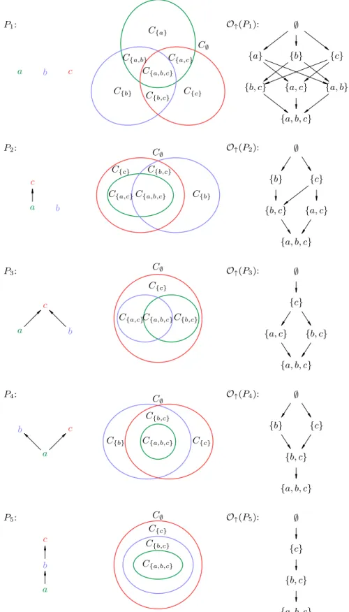
Figure A1. The poset of labels,P, the Venn diagram of the inclusion of sets Axfor the generic case, and the lattice of the labels of the intersections (classes) being not empty by construction, O↑(P), are shown for the five possible posets (up to permutation) of three labelsP={a, b, c}[30].
and top elements. Note that in the main text we use order ideals and filters,which are just the down- and up-sets. In the cases when the posets are lattices, lattice ideals and filters are considered automatically in the literature [21]. (Lattice ideals and filters are nonempty down- and up-sets which inherit (finite) joins and meets.) However, in our case, even when the posets considered are lattices, our construction always uses order ideals and filters.
If we consider a power set, the natural partial order is the set inclusion ⊆, then the meet∧ is the intersection∩, and the join∨is the union∪. For a poset P, O↓(P) andO↑(P) are lattices with respect to the inclusion. IfP is a lattice, then also O↓(P)\ {∅}andO↑(P)\ {∅}are lattices with respect to the inclusion.
Appendix A.2. Intersections of sets
Let us have a setA, and a finite number of its (different) subsetsAx∈2A, labelled by elementsx∈P in a label setP. All the possible intersections of the setsAx can be labelled by a subsetx∈2P as
Cx:= \
x0∈x
Ax0∩ \
x∈x
Ax∈2A, (A.1)
where the complement of the subset Ax is in 2A, that is, Ax0 = A\Ax0, while the complement of the subsetxis in 2P, that is, x=P\x. (We use the convention that the empty intersection is the whole setA, while the empty union is the empty set∅.
Note that, forAx0, there does not necessarily existx∈P such thatAx=Ax0.) We would like to exploit the possible inclusions of the subsetsAxin the labelling of the intersections. In order to do this, we endow the setPof the labels with a partial order, based on the inclusion of the subsetsAx:
∀y, x∈P : yx ⇐⇒ Ay ⊆Ax. (A.2) Lemma 14 In the above setting, we have that if Cx6=∅then x∈ O↑(P).
Proof: This can be proven contrapositively: Ifxis not an up-set (x∈ O/ ↑(P)), then there exists a pair of elements x∈ x and x0 ∈ x such that x x0, then Ax ⊆Ax0
by (A.2), thenAx0∩Ax=∅, thenCx=∅by (A.1).
Lemma 15 In the above setting, when S
x∈PAx =A, we have that if Cx 6=∅ then x∈ O↑(P)\ {∅}.
Proof: This is Lemma 14together with that in the case of the stronger assumption we have that ifCx6=∅ thenx6=∅. This, again, can be proven contrapositively: Let x=∅, thenC∅=T
x0∈PAx0 =S
x0∈PAx0 =A=∅, where (A.1) and De Morgan’s law
were used.
Examples can be seen in figureA1(note that the up-set lattice O↑(P) is drawn upside-down, which is intuitive in the case of correlation and entanglement theory).
Lemma14and Lemma15givenecessarycondition for the nonemptiness of the classes.
(If the condition does not hold, then the class can be calledempty by construction[10].) It is not sufficient, as one can see, for example, in figure A2: in the case when P is an anti-chain, it is possible thatAa 6⊆Ab, Aa 6⊆Ac, whileAa ⊆Ab∪Ac, leading to C{a}=Ab∩Ac∩Aa=∅(empty not by construction).
Earlier version of these results was shown in [10] in the special setting where it was used (P =PII∗). Note that the present formulation is more general, hereP does not have to be a lattice, and the setsAxdo not have to coverAentirely (S
x∈PAx⊆A).
a b c P1:
C{a,b,c}
C{b,c}
C{a,c}
C{a,b}
C{b} C{c}
C∅
∅
{a} {b} {c} {b, c} {a, c} {a, b}
{a, b, c} O↑(P1):
Figure A2. Example for a class (C{a}), which is empty, but not by construction.
(Compare with the first row of figureA1)
Appendix B. Multipartite quantum states Appendix B.1. Order isomorphisms for Level I-II
Proof of (3) and (6): The first inclusion in (3), υ ξ ⇔ Dυ−unc ⊆ Dξ−unc, was proven in Appendix A.4 in [10] forpureξ-separable (hence pureξ-uncorrelated) states only. For mixedξ-uncorrelated states, a slight modification is needed.
To see the “only if ” implication, let us have % ∈ Dυ−unc, then % = N
Y∈υ%Y = N
X∈ξ
N
Y∈υ,Y⊆X%Y
∈ Dξ−unc, where the first equality is (1); and at the second equality we have used the assumption υ ξ, which gives by definition that ∀Y ∈υ,
∃X ∈ ξ such that Y ⊆ X, making possible to collect the states of subsystems Y contained in a givenX, which can be done for all subsystemsX.
To see the“if ”implication, we prove the contrapositive statement,υ6ξ ⇒ Dυ−unc6⊆
Dξ−unc. Let us have % ∈ Dυ−unc, then, using the notation %X = TrL,X%, consider N
X∈ξ%X =N
X∈ξTrL,X%=N
X∈ξTrL,XN
Y∈υ%Y =N
X∈ξ
N
Y∈υTrY,X∩Y%Y = N
Y∈υ
N
X∈ξTrY,X∩Y %Y
6= N
Y∈υ%Y = %, where at the second and the last equalities we used the assumption that % ∈ Dυ−unc (we use the notation TrX,X0 = N
i∈X∩X0TrHi : LinHX → LinHX0 for the partial trace, when X0 ⊆ X); the third equality can be checked by the decomposition of tensors into linear combination of elementary tensors, and using the linearity of the partial trace and the tensor product;
the fourth equality is just the associativity of the tensor product. The nonequality comes from the assumption thatυ 6 ξ, which gives that ∃Y ∈υ for which ∀X ∈ ξ we haveY 6⊆X, then the termN
X∈ξTrY,X∩Y %Y 6=%Y for thisY, if%Y is not of the product form, which is an extra assumption, which can be fulfilled, since dimHi>1.
Thesecond inclusion in (3), υξ ⇔ Dυ−sep⊆ Dξ−sep, has already been proven in Appendix A.4 in [10].
The first inclusion in (6), υ ξ ⇔ Dυ−unc ⊆ Dξ−unc, was proven in Appendix A.8 in [10] for pure ξ-separable (hence pure ξ-uncorrelated) states only. For mixed ξ-uncorrelated states, the same steps can be applied.
Thesecond inclusion in (6), υξ ⇔ Dυ−sep⊆ Dξ−sep, has already been proven in
Appendix A.8 in [10].
Note that (3) and (6) immediately lead to that υ =ξ if and only if Dυ−unc = Dξ−unc,Dυ−sep = Dξ−sep, while υ = ξ if and only if Dυ−unc = Dξ−unc,Dυ−sep = Dξ−sep, since an order isomorphism is automatically bijective.