The multiple hierarchical legislatures in representative democracy ∗
Katsuya Kobayashi
†Attila Tasn´ adi
‡May 2, 2012
Abstract
Multiple hierarchical models of representative democracies in which, for instance, voters elect county representatives, county representatives elect district representatives, district representatives elect state representatives and state representatives a president, reduces the number of electors a representative is answerable for, and therefore, con- sidering each level separately, these models could come closer to direct democracy. In this paper we show that worst case policy bias increases with the number of hierarchical levels. This also means that the opportunities of a gerrymanderer increase in the number of hierarchical levels.
Keywords: Electoral systems, Median voter, Gerrymandering, Council democracies.
JEL Classification Number: D72.
1 Introduction
In many parliamentary democracies each representative is elected within a single-member district. Because of the huge difference in the number of representatives and the number of voters a representative is answerable for too many voters, which is problematic since this might lead to a misrepresentation of voters’ interests, lower participation rates among other negative effects. A possible extension of this model could reduce this huge difference by introducing intermediate levels with intermediate districts and representatives. Voters in the same single-member district would elect an intermediate representative, who grouped together
∗This project started when Kobayashi of Hosei University visited the Corvinus University of Budapest by the exchange program from February 20, 2012 through March 30, 2012. Kobayashi thanks the Corvinus University of Budapest for their financial support and their hospitality.
†Faculty of Economics, Hosei University, Tokyo, Japan. E-mail katsuyak@hosei.ac.jp
‡Department of Mathematics, Faculty of Economics, Corvinus University of Budapest, Budapest, Hungary.
E-mail attila.tasnadi@uni-corvinus.hu
with an appropriate number of other intermediate representatives into an intermediate single- member district could vote for one of the final representatives. Clearly, one can extend this model further by increasing the number of intermediate levels, and thus, obtaining a model of multiple hierarchical representative democracy.
In fact our suggested model can be basically found in the literature and they were, though not in its pure form, attempts for its implementation in the past one and a half century.
In expressing his views on democracy, Jefferson (1816) outlined a so-called ward system in which he distinguished between the national, the state, the county and the ward level. He characterized this system by
“It is by dividing and subdividing these republics from the great national one down through all its subordinations, until it ends in the administration of every man’s farm by himself; by placing under every one what his own eye may superintend, that all will be done for the best.”
The so-called council system is based on a similar idea (for its history, we refer to Olsen, 1997).
However, the council system only existed just formally, in the sense that contrary to its spirit it did not result in a democracy, but merely in a bureaucratic executing system of a totalitarian state. Though our real-life experiences with council systems are extremely negative, it still has its advocates like Arendt (1977).1 From another point of view understanding council systems may help us in understanding democracy as stated by Medearis (2004):
“An understanding of the council movement’s ideas and practices might have (and could still) contribute to an enrichment of democratic theory. ... The majority of movement participants did not reject parliamentary institutions, but attempted to achieve their democratizing goals in tandem with them, apparently envisioning an interplay between different social entities that would bring about the desired unleashing of democratic agency.”
We are not aware of a formal analysis proving why the council system might have gone wrong. In this paper, by extending the model of districting by Gilligan and Matsusaka (2006), we show that in the worst-case or in case of extreme gerrymandering a multiple hierarchical model of representative democracy can serve the interest of a minority. In particular, by increasing the number of intermediate levels we get closer and closer to a dictatorship. Con- cerning random districting the same results as obtained by Gilligan and Matsuasaka (2006) prevail for the multi-level hierarchical model of representative democracy. In particular, policy bias emerges with positive probability and expected bias equals zero in a symmetric setting, while in a skewed setting expected bias is also positive.
The remainder of the paper is organized as follows. Section 2 presents our extended model of multiple hierarchical representation and a motivating example. Section 3 considers the
1For a discussion of Arendt’s work see, for instance, Isaac (1994).
worst case bias, which can emerge by coincidence or in case of an optimal gerrymandering.
Section 4 investigates random districting. Finally, we conclude in Section 5.
2 The model
We use a multiple application of the median voter theorem by extending Gilligan & Mat- susaka’s model that is a double application of it. According to the median voter model introduced by Black (1958) which is well known, the policy which the median voter prefers prevails over any other policies in case of a uni-dimensional policy space and single-peaked preferences of voters.
Gilligan & Matsusaka define and calculate a bias between the median policy and the policy decided in the legislature composed of representatives elected in single-member districts, where each voter is allocated to exactly one district. They mention that there is a possibility for gerrymandering in the indirect democracy that is to divide voters into districts for giving one group an advantage in the election, and that as a result, the final policy chosen by representatives in the legislature may be away from the policy the median voter prefers.
As we pointed out in the introduction, the political system in which the policy is decided hierarchically is adopted in some societies. In this paper, by extending Gilligan & Matsusaka’s model, more accurately extending the median voter theorem vertically, we will show in the following part how the final policy, which the representative being finally elected in “multiple levels legislatures” chooses and implements, is decided in gerrymandered districts and we will show how the final policy can deviate from that of the median voter theorem.
Basically, the settings and notations of our model are similar to Gilligan & Matsusaka’s model. The population of citizens consists of N assumed as an odd number of people, all of them vote, and they are called voters hereafter, so that the voters set is defined as N = {1,2,3, . . . , N}. We assume that each voteri∈ N has an ideal policy at own position xi ∈R, and that each voter’s utility decreases strictly monotonically as an implemented policy is getting farther away from its own ideal position. Then the median of all voters is voter
N+1
2 . We also assume that voters with smaller numbers (the left wing from the median) are more liberal and that those with larger numbers (the right wing from the median) are more conservative for convenience. Thus we denotex1 ≤x2 ≤. . .≤xN. LetF(x) be the cumulative distribution function of voter ideal points. We assume there is a unique median voter in the population with ideal pointx∗P OP such thatF(x∗P OP) = 12. The distance of a policyxfrom the median of all voters is called a bias, which we define below in an analogous way to Gilligan &
Matsusaka:
Definition 1. The measure of a policy bias equals B =|F(x)−F(x∗P OP)|.
Observe that policy choice x is unbiased or has minimal bias when B = 0, and x has maximal bias when B = 1/2.
We considert+1 decision levels starting fromt = 0. On each decision leveli∈ {1,2, . . . , t, t+
1}voters grouped into equally sized districts send a representative to the next, thei+ 1-th de- cision level. On thet-th decision level, representatives are elected and sent to thet+ 1 decision level, which is the final decision level. On the t+ 1-th decision level, only one representative who decides the final policy is elected. We assume that none of the representatives can make a binding commitment regarding the final policy so that the final representative choses and implements its most favored policy, that is its own ideal policy.
Since now we are considering hierarchical legislatures composed of representatives elected among voters, the above decision process can also be described in the following way: the lowest decision level consists of the voters, the second decision level is legislature 1, the third decision level is legislature 2, and so on. Finally the t-th decision level is legislature t − 1, and the t + 1-th decision level is legislature t that is composed of only one district and that elects only one representative who is called the final representative. Thus t means the number of hierarchical legislatures inserted between voters and the final representative, which are like ward representatives, county representatives, state representatives and the national representatives.
Each legislature is composed of representatives as follows. LetKi be the number of districts on thei-th decision level, i∈ {0,1,2, . . . , t, t+ 1}. Since on thet+ 1-th decision level there is only one district, we letKt+1 = 1. We assume single-member districts, consequentlyKi is also the number of representatives in legislature i on the i+ 1-th decision level. For convenience, let K0 = N when t = 0. Thus in case of t = 0 only one representative is elected directly among the voters, who implements the final policy, that is viewed as the direct democracy.
When t ≥ 1, our model becomes an indirect democratic system, especially when t ≥ 2, it has hierarchical multiple decision levels, namely hierarchical legislatures with multi-levels. We assume that these representatives on each decision level are elected among voters or repre- sentatives in districts of one level below by a majority rule. We also assume that every voter and representative on eachi-th decision level cast a ballot sincerely and then only one among them is elected as a single-member district representative. Consequently the median voter of each district is elected as the representative. Thus the legislature on thei+ 1-th decision level is composed of the median voters from each district from a level below. Since every district on the same level is assumed to have the same size, the population of each district on thei-th decision level equals Ki/Ki+1. Since usually the numbers of districts in upper legislatures are smaller than those in lower legislatures, Ki ≤Kj, i > j is assumed.
The basic structure of our model is like the following. First,N voters divided in K1 equal- sized districts with N/K1 =K0/K1 voters on the first decision level elect the representatives of legislature 1 on the second decision level, consequently K1 representatives are in legislature 1. Second, the representatives of legislature 1 divided in K2 equal-sized districts withK1/K2 members elect the representatives of legislature 2 on the third decision level, consequently K2 representatives are in legislature 2. Third, the representatives of legislature 2 divided
in K3 equal-seized districts with K2/K3 members elect the representatives of legislature 3 on the forth decision level, consequently K3 representatives are in legislature 3, and so on.
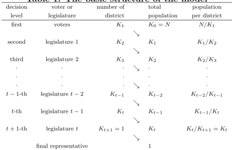
Finally, since the t+ 1-th decision level is the final one and Kt+1 = 1, the Kt representatives in legislature t on the t + 1-th decision level elect only one representative who is the final representative. The representative decides and implements only one policy, which is a number on the real line, applying to all voters. Table 1 depicts the above structure. Here, since all voters and representatives cannot commit to policies at all, the final representative implements its own ideal policy. We can say that Gilligan & Matsusaka’s model is the special case oft= 1 in our model. Since every districts is equal-size at each level, there is no disparity in the number of voters per representation.
Table 1. The basic structure of the model
decision voter or number of total population
level legislature district population per district
first voters K1 K0=N N/K1
&
second legislature 1 K2 K1 K1/K2
&
third legislature 2 K3 K2 K2/K3
· · · & · ·
· · · · ·
· · · & · ·
t−1-th legislaturet−2 Kt−1 Kt−2 Kt−2/Kt−1
&
t-th legislaturet−1 Kt Kt−1 Kt−1/Kt
&
t+ 1-th legislaturet Kt+1= 1 Kt Kt/Kt+1=Kt
&
final representative 1
From the above structure, we can immediately obtain the lemma below:
Lemma 1. The number of hierarchical levels is at most the number of prime factors of N. Proof. We will prove this by contradiction. Let N = a1 ·a2 ·a3· · ·at, where each ai, i ∈ {1,2,3, . . . , t}, is a prime factor ofN. We assume that for givenN we can makej+ 1 decision levels, noting Kj+1 = 1, where j > t. Then the populations of each district on each of level 1,2,3, . . . , j are KN
1,KK1
2,KK2
3, . . . ,KKt−1
t , . . . ,KKj
j+1, respectively, where Kj+1= 1. Thus N = N
K1
· K1 K2
·K2 K3
· · ·Kt−1
Kt
· · · Kj Kj+1
,
and the number of the factors of N is j+ 1. However, N cannot be the product of more than t numbers from its prime factorization; a contradiction.
At first sight it might look like that Lemma 1 imposes a severe restriction on the number of possible decision levels in our hierarchical model of representative democracy. For instance, if N is a prime number, we can construct only one district on the first decision level, accordingly t = 0 emerges as the only possible case because of the assumption of equal-sized districts.
We can overcome this problem by allowing for almost equal-sized districts, that is rounding either down or up value Ki/Ki+1, and picking consistently one of the two electors from “the middle” in the case of even district sizes, so that the district sizes can be different on the i-th decision level from each other. In this case, some disparities in the number of voters per representation occur on the i-th decision level. However, this extension would just complicate our analysis without substantial gain, and therefore we assume that Ki/Ki+1 are integers for alli = 0,1, . . . , t−1, t, whereK0 =N, and that districts of all levels have an odd number of voters.
Let x∗i+1,k be the ideal point of the median representative or voter in district k on the i+ 1-th decision level that is legislaturei. Since one district is on the final decision level, that is Kt+1 = 1, the policy outcome decided in the final legislature becomes x∗t+1,1.
In the next example, we will exhibit how far away the final policy in the multiple hierar- chical electoral system in case of extreme gerrymandering can be from the policy decided in the direct democracy, that is the median voter’s ideal policy, and we will also compare the final policy in our model with that in Gilligan & Matsusaka’s model in the next example.
Example 1. We will consider an example of three hierarchical legislatures where t+ 1 = 3, N = 27, voters set N ={1,2,3, . . . ,25,26,27} and voters have different ideal points, that is x1 < x2 < . . . < xN. We will compare the indirect democracies of two decision levels (t = 1) and three decision level (t= 2) with the direct democracy (t = 0). 2 In this case, the median voter is N+12 = 14 as shown in Table 2, so that the final policy is decided atx∗1,1 =xP OP = 14 in the direct democracy.
Table 2. The case of N = 27, K1 = 1
{1,2,3,4,5,6,7,8,9,10,11,12,13,14,15,16,17,18,19,20,21,22,23,24,25,26,27}
↓ 14
However, as Gilligan & Matsusaka is showing, the final policy is not always decided at the median of voters with gerrymandered districts in the indirect democracy. We will exhibit that the selected policy is decided at the father away from the median of voters as the levels of delegation increase in this example. The Table 3 and Table 4 illustrate the most extreme gerrymandering to give advantage to the liberal (left) voters in the case of two decision levels (t= 1), which can be regarded as regular indirect democracies, where the legislature composed of the representatives elected in single-member districts decides the final policy.
How do liberal voters gerrymander for maximizing their own political payoff? We shall assume that a liberal extremist who is voter-1, hereafter called “she”, can arrange all districts
227 equals 3·3·3 by the prime factor decomposition. From this, in case of two decision levels, each district on the first decision level and that on the second level are composed of 9 voters and 3 representatives, respectively, or of 3 and 9, respectively. In case of three decision levels, each district is composed of three voters or representatives on every decision level. As a result, we can obtain combinations of K1 = 1, (K1, K2) = (3,1),(9,1) and (K1, K2, K3) = (9,3,1) for the one decision level case, the two decision levels case and the three decision levels case, respectively.
without loss of generality. 3 Then she will attempt to put the median of all representatives in each district on each decision level on a position being as left as possible. In this paper, we use the well-known “cracking and packing” algorithm as it is formulated by Gilligan &
Matsusaka of which the explanation is in the following quotation for each discrete voter with an ideal point on the real line:
“first, citizens with high-value ideal points are “cracked” into districts where they are the minority, maximizing the influence of citizens with low-value ideal points, and second, the remaining high value citizens are “packed” into districts contain- ing a preponderance of like-minded citizens in order to waste their votes through overkill.”
For t = 1 and N = 27 we can consider two cases, where (K1, K2) = (3,1) and (9,1).
Then we can easily find the policies that are as close as possible to voter-1 who is the liberal extremist like in the example with nine voters in Gilligan & Matsusaka. In both Tables 2 and 3, the policies are decided by voter-10 whose ideal position is 4 positions away from the median voter. Even if there are several districts patterns in a combination of N and t, it can be shown that the maximum distances between the final policies and the median in the case of an optimal gerrymandering for either the liberal or conservative extremists who are
“partisan”s remain identical.
Table 3. The case of N = 27, K1 = 3, K2 = 1
{1,2,3,4,5,24,25,26,27} {6,7,8,9,10,20,21,22,23} {11,12,13,14,15,16,17,18,19}
↓ ↓ ↓
{5 10 15}
↓ 10
Table 4. The case of N = 27, K1 = 9, K2 = 1
{1,2,27} {3,4,26} {5,6,25} {7,8,24} {9,10,11} {12,13,14} {15,16,17} {18,19,20} {21,22,23}
↓ ↓ ↓ ↓ ↓ ↓ ↓ ↓ ↓
{2 4 6 8 10 13 16 19 22}
↓ 10
Finally, what is the policy decided by the upper representatives if an additional level of representation is incorporated in the above policy decision process in case of gerrymandering?
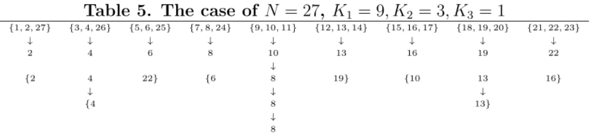
In the same way as in our previous two decision levels examples, the districts on the second decision level are arranged by one liberal extremist in order to enforce the final policy coming as close as possible to her own ideal point. In case of three decision levels the districts pattern is only (K1, K2, K3) = (9,3,1). Table 5 illustrates the case. The policy is decided by voter-8 who is even father away from the median than in the case of two decision levels, that is 6 positions away from the median.
3Of course, in the same way we can also consider a conservative extremist instead of a liberal extremist.
Table 5. The case of N = 27, K1 = 9, K2 = 3, K3 = 1
{1,2,27} {3,4,26} {5,6,25} {7,8,24} {9,10,11} {12,13,14} {15,16,17} {18,19,20} {21,22,23}
↓ ↓ ↓ ↓ ↓ ↓ ↓ ↓ ↓
2 4 6 8 10 13 16 19 22
↓
{2 4 22} {6 8 19} {10 13 16}
↓ ↓ ↓
{4 8 13}
↓ 8
As a result, this example is suggesting that the final policy decided by the representative becomes a farther away position from the median of all voters as hierarchical decision processes are added in the democratic representative system in case of many voters. Indeed, we will mention this fact generally in Proposition 1 in the next section. Additionally, from the result of Lemma 1, many voters are required to construct a higher hierarchical representative system since we can only construct the decision levels within the number of prime factors of voters number, N, at most. Actually, in this example where N = 27, the liberal extremist can construct only three decision levels at most, consequently she can slide the final policy to the left side by only 6-position from the median voter’s position. Thus this example is also suggesting that an extreme voter needs so many other voters in order to obtain an political advantage by gerrymandering. We will also show this fact generally in Corollary 2 in the next section.
3 Worst case bias or liberal optimal gerrymandering
From Example 1 we can conjecture that the final policy outcome is getting farther from the median of all voters as we add more hierarchical levels of legislatures, when all districts on each level are arranged by a liberal extremist’s gerrymandering. The below lemma determines the policy position finally decided in the case oft+1 decision levels, namely the policy position is decided in a political decision system composed of both all voters and t+ 1 hierarchical legislatures including the final representative in the indirect democracy.
Lemma 2. (Generalization of Gilligan & Matsusaka (2006)) In case of liberal ger- rymandering the policy outcome decided by the political decision system composed of t+ 1 hierarchical decision levels is
x∗t+1,1 = 1 2
1 2
t
1
KtKt−1· · ·K2K1(Kt+1)(Kt+Kt−1)(Kt−1+Kt−2)· · ·(K2+K1)(K1+N). (1) Proof. (1) will be proved by the induction.
(I) Suppose t = 0. This case is the direct democracy case with no legislature. When t= 0, in the right-hand side of (1), both K 1
tKt−1···K2K1 and (Kt+Kt−1)(Kt−1+Kt−2)· · ·(K2+ K1)(K1+N) include no terms. Thus (1) becomes
x∗1,1 = 1 2
1 2
0
(K0+ 1) = N + 1 2 .
This is consistent with the median of all voters.
(II) Suppose t = 1. This case is already proved in Proposition 1 of Gilligan & Matsusaka (2006).
(III) Suppose, when t =n, (1) is correct. Then it is sufficient to show that (1) is correct when t=n+ 1. We can transform (1) at t=n to
x∗n+1,1 = Kn+ 1 2
| {z }
median ofn+1-th level
1 2
Kn−1 Kn + 1
| {z }
n-th level
1 2
Kn−2 Kn−1
+ 1
| {z }
n−1-th level
· · ·1 2
K1 K2 + 1
| {z }
second level
1 2
N K1 + 1
.
| {z }
first level
This formula means the following: the last term is the median of the first district on the first decision level, the second term from the last is the median of the first district on the second decision level, and so on. Finally the first term is the term to indicate the Kn2+1-th representative on the n+ 1-th decision level at which there is only one district. By this term, the median in the district on the n+ 1-th decision level is indicated.
Here when t=n+ 1, the final decision level is the n+ 2-th, and Kn+1 representatives are on the n+ 2-th decision level. Thus, noting that Kn+2 = 1, the median representative on this decision level is 12(KKn+1
n+2+ 1) = Kn+12+1 that is changed from Kn2+1 of the median on then+ 1-th decision level. Thus since for t =n+ 1 the Kn representatives on the n+ 1-th decision level have to be grouped into Kn+1 districts, x∗n+2,1 has to be multiplied by 12(KKn
n+1 + 1)· KKn+1+1
n+1 . Then we can obtain
x∗n+2,1 = x∗kn+1,1 ·1 2
Kn
Kn+1 + 1
· Kn+1+ 1 Kn+ 1
= Kn+ 1 2
1 2
Kn−1
Kn + 1 1
2
Kn−2
Kn−1
+ 1
· · ·
· · ·1 2
K1 K2 + 1
1 2
N K1 + 1
1 2
Kn Kn+1 + 1
Kn+1+ 1 Kn+ 1
= 1
2 1
2 n+1
1
Kn+1Kn· · ·K2K1(Kn+1+ 1)(Kn+1+Kn)(Kn−1+Kn−2)· · ·
· · ·(K2 +K1)(K1+N) This formula is (1) at t=n+ 1 exactly.
Lemma 2 is the case of the most extremely liberal gerrymandering with t+ 1 decision levels. Of course, we can also obtain an analogous result for the most extremely conservative gerrymandering. Additionally, from the proof of Lemma 2, (1) is also indicating the policy position in the direct democracy at t = 0. Concerning the final policy position, the direct democracy can be viewed as a special case of a hierarchical political system.
Incidentally, we can use the result of Lemma 2 to explain the partisan voters effect like one of Gilligan & Matsusaka’s applications: how many partisan voters are needed in order to implement their favorite policy in the legislature on the top-level by gerrymandering.
In our model, we rearrange all voters to those who are supporting a policy of xi ∈ {0,1}, namely the set of voters’ ideal points isN ={0,0,0, . . . ,0,1,1,1, . . . ,1}, where the population
of voters is still N. Let voters who prefer 0 be called partisan. Then, how many partisan voters are needed at least? This problem can be solved backwardly. Note that only one representative is on the t + 1-th decision level, that is Kt+1 = 1. First, one of partisans need to become the final representative to implement their favorite policy. Second, since the partisan final representative is elected from legislature t on the t+ 1-th decision level, they need a majority of the legislators in legislature t, that is at least
Kt Kt+1+1
2 = Kt2+1 electors because of Kt+1 = 1. Third, since each representative of legislature t on the t+ 1-th decision level is elected in a district in legislature t−1 on the t-th decision level, partisans need a majority of representatives in a majority of districts in legislaturet−1, that is at least
Kt−1
Kt +1
2
representatives in at least Kt2+1 districts on the t-th decision level, consequently they need
Kt−1
Kt +1
2
Kt+1
2 representatives in legislaturet−1 to have a majority in legislaturet. Forth, since each representative in legislature t− 1 on the t-th decision level is elected in a district in legislature t−2 on the t−1-th decision level, partisans need a majority of representatives in a majority of districts in legislature t−3, that is at least
Kt−2 Kt−1+1
2 representatives in at least
Kk−1
Kt +1
2
Kt+1
2 districts on thet−1-th decision level, consequently they need
Kt−2 Kt−1+1
2
Kt−1
Kt +1
2
Kt+1 2
representatives in legislature t−2 to have a majority in legislature t−1. The same logic is continuing until the voters level. Then we can obtain the same formula as (1) by using the same transforming in the proof of Lemma 2. Thus the next corollary can be obtained:
Corollary 1. The minimum population of partisans in voters is 1
2 1
2 t
1
KtKt−1· · ·K2K1(Kt+ 1)(Kt+Kt−1)(Kt−1+Kt−2)· · ·(K2+K1)(K1+N) in order that the final policy becomes partisans’ favorite policy by their gerrymandering in the hierarchical system with t+ 1 decision levels.
This corollary can also be obtained by applying the “crack and pack” method at each level. As Gilligan & Matsusaka is mentioning “majority-minority”, Corollary 1 and Lemma 2 require strictly optimal gerrymandering for minorities to implement a policy they prefer.
To put it another way, if a liberal extremist has the authority to arrange all districts in each level and if liberal voters are minorities in all voters, in any levels the extremist should not make super-majority minorities districts where the minorities have super-majorities in a few districts. Even if it might seem partially good for minorities to make a few districts composed of super-majority minorities, particularly if the final policy is decided in proportion to the number of representatives on the t + 1-th decision level, it actually prevents the minorities from their favorite policy even in the system with the multiple decision levels where they need fewer liberal voters than in the single level legislature by gerrymandering.
In Lemma 2, (1) can be obtained as the final policy being the nearest to the extremist in the left side. From this result, as the characterization of the formula, the next proposition says the monotonicity of alienation in the hierarchical legislatures.
Proposition 1. The final policy is getting farther away from the median of voters monotoni- cally as the number of hierarchical stages increases.
Proof. We calculate the ratio of x∗t+1,1 and x∗t+2,1. x∗t+1,1
x∗t+2,1 =
1 2
1 2
t 1
KtKt−1···K2K1(Kt+ 1)(Kt+Kt−1)(Kt−1+Kt−2)· · ·(K2+K1)(K1+N)
1 2
1 2
t+1 1
Kt+1Kt···K2K1(Kt+1+ 1)(Kt+1+Kt)(Kt+Kt−1)· · ·(K2+K1)(K1+N)
= Kt+ 1
1 2
1
Kt+1(Kt+1+ 1)(Kt+1+Kt)
= 2Kt+1(Kt+ 1) (Kt+1+ 1)(Kt+1+Kt)
Here, since ∀t ∈ {1,2,3, . . . , n}, Kt ≥ Kt+1, 2Kt+1(Kt + 1) − (Kt+1 + 1)(Kt+1 + Kt) = (Kt+1−1)(Kt−Kt+1)≥0, so that the numerator is always more than the denominator. Thus
xkt+1,1
xkt+2,1 ≥1.
For a given number of voters N and a given number of levels t we determine the number of districts K1, . . . , Kt that may result in the most biased outcome. Noting that K0 =N, the next proposition can be obtained.
Proposition 2. In the case of N voters and t+ 1 decision levels, the multi-level districting given by
∀i= 1, . . . , t, t+ 1 :Ki =Nt−(i−1)t+1 (2) admits the largest possible bias.
Proof. Determining maximum bias is equivalent with minimizing x∗t+1,1/N with respect to K1, . . . , Kt. In the next formula
x∗t+1,1
N =
1 2
t+1
1
KtKt−1· · ·K2K1K0(Kt+1)(Kt+Kt−1)(Kt−1+Kt−2)· · ·(K2+K1)(K1+K0), we multiply 1/K0,1/K1, . . . ,1/Kt to the terms from the last in the reverse order. Hence, we have to minimize expression
1 2
t+1 1 + 1
Kt 1 + Kt Kt−1
· · ·
1 + K2
K1 1 + K1 K0
(3) yielding first-order conditions equivalent with
0 =−Ki+1 Ki2
1 + Ki Ki−1
+
1 + Ki+1 Ki
1 Ki−1
for all i= 1, . . . , t; from which we can obtain by simple rearrangements
Ki+1Ki−1 =Ki2 (4)
for alli= 1, . . . , t, whereKt+1 = 1. It can be verified that the first-order conditions determine the minimum value for expression (3).
We claim that
Kt−(i−1) = (Kt−i)i+1i (5)
for all i = 1, . . . , t, which we prove by induction. Clearly, our claim holds true for i = 1 by equation (4). Assume that (5) is valid foriand we show that it also holds true fori+ 1. From (4) we have
Kt−i+1Kt−i−1 = (Kt−i)2, and by employing our induction hypothesis we get
(Kt−i)i+1i Kt−i−1 = (Kt−i)2 ⇔ Kt−i = (Kt−i−1)i+1i+2, which is what we wanted to show.
Finally, by employing (5) recursively we obtain the statement of our proposition.
In fact Proposition 2 describes the hierarchical structure of a multi-level gerrymandering.
Our next corollary determines the respective worst case bias.
Corollary 2. If the number of levelstis fixed, then as the number of votersN tends to infinity worst-case bias approaches
F x∗t+1,1
−F (x∗P OP) = 1
2 − 1
2 t+1
Proof. From (5) one obtains
Kt−(i−1)
Kt−i
= 1
(Kt−i)i+11
. (6)
By substituting (6) into (3) and letting N tend to infinity, we obtain our corollary.
Now by increasing the number of levels t maximum bias approaches its highest possible level, which we state in the next corollary.
Corollary 3. Asttends to infinity maximum worst-case bias in case of liberal gerrymandering tends to x∗P OP −x1.
In particular, if party A is at the left end and party B on the right end of the unit interval, then, for instance, party A’s most preferred outcome will be the national outcome independently form the voters preferences.
4 Random districting
One may hope that the extent of the worst case bias shown in the previous section will not cause a severe problem because, for instance, random districting (that is, voters are randomly grouped into districts) could solve the problem. However, in this section we show that the results on random districting obtained by Gilligan and Matsusaka (2006) remain valid for our multiple hierarchical model of representative democracy.
First, assume thatN is odd,dN/2e+ 1 voters have their ideal points at 1 andbN/2cvoters have their ideal points at 2.4 We assume again for simplicity that the number of voters N takes a value such that for givenK1, . . . , Ktat-level districting can be carried out in integers.5 The median voter’s ideal point equals 1. However, one can group the voters into equally sized first-level districts such that the ideal point of the first-level median representative equals 2, which means that we have more first-level districts with a median representative at 2 than at 1.
Now on the second-level one can also construct a districting having more representatives with ideal points 2 than 1. We can proceed in the same way until we arrive at the top level, which then has a median representative with ideal point 2. Since these type of districting emerge with positive probability the expected ideal point will exceed the voters’ median point.
In the described example voters’ ideal points are a bit skewed. The next Proposition, which is analogous to Proposition 2 of Gilligan and Matsusaka (2006), investigates the cases of symmetric and up-wards skewed distribution of voters’ ideal points.
Proposition 3. Assuming that each districting is equally probable, the expected bias of random districting
1. is zero if the voters’ ideal points are symmetrically distributed around their median, and 2. is biased up-wards if the voters’ ideal points are skewed up-wards.
Proof. Assume that the voters’ ideal points are ordered increasingly, i.e. x∗1 ≤x∗2 ≤. . .≤x∗N. Let M = (N + 1)/2. We shall denote by the p(xi) the probability that voter i becomes the top-level representative, that is, policy-maker or legislator.
We start with proving point 1. Because of the symmetric setting we must have p(xM−i) = p(xM+i) and xM −xM−i =xM+i−xM for all i= 0, . . . , M −1. Hence,
E(x∗LEG) =
N
X
i=1
p(xi) =
M−1
X
i=1
p(xM−i)xM−i +p(xM)xM +
M−1
X
i=1
p(xM+i)xM+i =xM. (7) For establishing point 2, we just have to replacexM−xM−i =xM+i−xM withxM−xM−i ≤ xM+i−xM for alli= 0, . . . , M−1, which holds since the distribution of ideal points is up-wards skewed, in equation (7).
5 Concluding remarks
In this paper we introduced a multiple hierarchical model of representative democracy in the hope that it might result in a “more direct” democracy since the connections between a rep- resentative and its voters can be strengthened by the fact that a representative is answerable for less voters as the number of hierarchical levels increases. However, instead of supporting
4This example is an extension of an example by Gilligan and Matsusaka (2006, p. 387).
5Hence, each district has a uniquely determined median voter.
evidence for our hierarchical model we found its increased vulnerability to gerrymandering and policy bias. This might contribute to a formal explanation to why the attempts of imple- menting hierarchical models of representative democracy in the past failed and contribute to a better understanding of representative democracy.
In future research we plan to investigate random districting further and introduce infor- mational structures into our model such as the verifiability of representatives behavior and the privacy of individual votes.
References
[1] Arendt, H. (1977): On Revolution. New York: Penguin.
[2] Black, D. (1958): The Theory of Committees and Elections. Cambridge: Cambridge University Press.
[3] Buchanan, J.M., Tullock, G. (1962): The Calculus of Consent: Logical Foundations of Constitutional Democracy. Ann Arbor, MI: Univeristy of Michigan Press.
[4] Gilligan, T.W., Matsusaka, J.G. (2006): Public Choice Principles of Redistricting.Public Choice 129, 381–398.
[5] Isaac, J.C. (1987): Oases in the Desert: Hannah Arendt on Democratic Politics. The American Political Science Review 88, 156–168.
[6] Jefferson, T. (1816): Letter to Joseph C. Cabell. In: Kurland, P.B., Lerner, R.
(eds.) The Founders’ Constitution, Volume 1, Chapter 4, Document 34, http://press- pubs.uchicago.edu/founders/documents/v1ch4s34.html, The University of Chicago Press (2000).
[7] Medearis, J. (2004): Lost or Obscured? How V. I. Lenin, Joseph Schumpeter, and Hannah Arendt Misunderstood the Council Movement. Polity 36, 447–476.
[8] Olson, J. (1997): The Revolutionary Spirit: Hannah Arendt and the Anarchists of the Spanish Civil War. Polity 29, 461–488.