The Multiple Hierarchical
Legislatures in a Representative Democracy: Districting for Policy Implementation
by
Katsuya Kobayashi, Atilla Tasnádi
C O R VI N U S E C O N O M IC S W O R K IN G P A PE R S
http://unipub.lib.uni-corvinus.hu/1774
CEWP 19 /2014
The Multiple Hierarchical Legislatures in a Representative Democracy: Districting for Policy Implementation
Katsuya Kobayashi
∗Attila Tasn´ adi
†December 17, 2014
Abstract
We build a multiple hierarchical model of a representative democracy in which, for instance, voters elect county representatives, county representatives elect district repre- sentatives, district representatives elect state representatives, and state representatives elect a prime minister. We use our model to show that the policy determined by the final representative can become more extreme as the number of hierarchical levels increases be- cause of increased opportunities for gerrymandering. Thus, a sufficiently large number of voters gives a district maker an advantage, enabling her to implement her favorite policy.
We also show that the range of implementable policies increases with the depth of the hierarchical system. Consequently, districting by a candidate in a hierarchical legislative system can be viewed as a type of policy implementation device.
Keywords: Electoral Systems, Median Voter, Gerrymandering, Council Democracies.
JEL Classification Number: D72.
∗Faculty of Economics, Hosei University, 4342 Aihara-machi, Machida-shi, Tokyo 194-0298, Japan. E-mail katsuyak@hosei.ac.jp
†MTA-BCE “Lend¨ulet” Strategic Interactions Research Group, Department of Mathematics, Faculty of Eco- nomics, Corvinus University of Budapest, F¨ov´am t´er 8, Budapest H-1093, Hungary. E-mail attila.tasnadi@uni- corvinus.hu
1 Introduction
In many parliamentary democracies, each representative is elected within a single-member district. However, although having many citizens elect one representative may mean a govern- ment is elected efficiently, the relationship between a representative and his/her voters could be weak. This can result in a misrepresentation of citizens’ diverse interests, many wasted votes, and lower participation rates. Shugart and Carey (1992) point out that there are trade- offs between the efficiency of citizens’ choosing one government and the representativeness of their diverse interests. To reduce this misrepresentation, an electoral system in which a small number of citizens elect one representative can be better than a system in which many citizens elect one representative. While the former system is effective in avoiding misrepresentation, if there are many citizens, they need to be grouped into districts. Then, the system needs to form legislatures, councils, or assemblies comprising the elected representatives as efficiently as possible. However, a legislature may still have too many representatives, making it difficult to organize a single government (e.g., by electing a prime minister). In this case, both efficiency and representativeness may be improved by forming an upper legislature comprising a few rep- resentatives from those in the legislature. Depending on the number of citizens, it may then be necessary to add further levels, thus creating a multiple hierarchical legislature. Here, citizens in the same single-member district elect an intermediate representative. Clearly, we can extend this system further by increasing the number of intermediate levels, thus obtaining a multiple hierarchical representative democracy. The purpose of this study is to determine the possible policy outcomes in such a system.
According to their constitution, China is an example of a representative democracy with a multiple hierarchical legislative system, as described above. The legislative system has four- levels, namely the nation, provinces, counties/cities/municipal districts, and townships/towns, with a government at each level. Representatives of legislatures at the national and provincial levels are elected by the legislatures at the next lower level (Article 97 in the Constitution of the People’s Republic of China).1 However, since the central and local governments, including each
1Initially, representatives at the county level were also elected by the legislatures at the next lower level. In
legislature, are “under the leadership of the Communist Party” (Preamble of the Constitution) in China, the party controls all elections (Institute of Chinese Affairs 2011).
The proposed model can also be found in related literature and attempts have been made to implement it during the past one and a half centuries, although not in its pure form. In expressing his views on democracy, Jefferson (1816) outlined the so-called “ward republics,”
in which he distinguished between the national, the state, the county, and the ward level. He characterized this system as follows:
“It is by dividing and subdividing these republics from the great national one down through all its subordination, until it ends in the administration of every man’s farm by himself; by placing under every one what his own eye may superintend, that all will be done for the best.”
The so-called council system is based on a similar idea (for its history, we refer to Olson (1997)).
However, even if the problems of misrepresentation or wasted votes are solved by districting citizens prior to an election, there is another potential problem: who groups citizens into districts? Should it be the incumbent representatives, citizens, or perhaps an outsider? If the district maker has a particular political position, she may construct the districts in such a way as to give an advantage to those candidates who have a similar political position to hers. This is referred to as “gerrymandering,” and can cause misrepresentations. Gilligan and Matsusaka (2006) measure how misrepresentative a policy determined in the single level legislature is in the case of most extreme gerrymandering. On the other hand, Coate and Knight (2007) show the conditions necessary for socially optimal districting when the independents’ policy positions are determined stochastically. From the standpoint of democracy, gerrymandering can be viewed normatively as one of the worst results. However, it can also be viewed as a type of implementation that provides district makers or social planners with a method of implementing their favorite policy.
the reform of the electoral law in 1979 (this change was also reflected in the Constitution in 1982), citizens’
direct election was expanded (Institute of Chinese Affairs 1980 and 1983). Since then, representatives at the county level have been elected by citizens directly, in addition to the township/town levels.
In this paper, we extend the districting model of Gilligan and Matsusaka and show that, by extreme gerrymandering, a multiple hierarchical model of a representative democracy can serve the interests of a minority. In particular, we show that as the number of voters increases, the district maker can construct more intermediate levels. Accordingly, the district maker’s policy implementability becomes stronger and, even in the case of an extreme political position, gains dictatorial power.2 In addition, we explicitly show the policy range that can be implemented by the hierarchical gerrymandering of every level. From these results, when each voter has the right to become the district maker with an equal probability, the most probable policy is the same as the case of gerrymandering by the extremists. We conclude that gerrymandering districts can be regarded as a method available to a district maker to implement her favorite policy.
In addition, her policy implementability is stronger when the legislative system is hierarchical, and is far stronger when there are many citizens in the society. Furthermore, our results may indicate why, despite the advantages pointed out by Jefferson, we find so few historical examples of a multiple hierarchical legislative system such as the ward republic, other than that of China, since the system gives stronger policy implementability to the district maker.
It is worthwhile mentioning that we abstract away from inherent geographical constraints, which pose a problem in the political districting problem. For works on measuring district compactness, we refer the reader to Chambers and Miller (2010, 2013) and Fryer and Holden (2011). In a normative framework, geographical constraints are considered by Puppe and Tasn´adi (2014), as well as the references therein. Details on redistricting in practice can be found, for instance, in Altman and McDonald (2010).
The remainder of the paper is organized as follows. Section 2 presents our extended model of a multiple hierarchical representation and a motivating example for the case of an extreme dis- trict maker. Section 3 considers the extremists’ policy implementability in the case of optimal gerrymandering. Then, Section 4 investigates the policy implementability by politically mod- erate district makers’ gerrymandering. Finally, Section 5 concludes the paper and applications of our model are provided in the Appendix.
2On this point, Galam and Wonczak (2000) use a numerical simulation to show that a dictatorship can appear under a hierarchical election. In contrast, we derive more general analytical results along a real line.
2 The model
We use a multiple application of the median voter theorem by nesting Gilligan and Matsusaka’s model into itself a finite number of times. According to the well-known median voter model introduced by Black (1958), the policy preferred by the median voter prevails over any other policies in the case of a uni-dimensional policy space and voters’ single-peaked preferences.
Gilligan and Matsusaka define and calculate the bias between the median policy and the policy decided in the legislature, which is composed of representatives elected in single-member districts, where each voter is allocated to exactly one district. They find that there is a possibil- ity for gerrymandering in an indirect democracy that divides voters into districts and gives one group an advantage in the election. As a result, the final policy chosen by the representatives in the legislature may not be the policy the median voter prefers.
As we pointed out in the introduction, some societies can adopt a political system in which policies are decided hierarchically. In this paper, by extending the model of Gilligan and Matsusaka, we show how the final policy chosen and implemented by the representative elected from the “multiple-level legislatures” is decided in gerrymandered districts. In addition, we show how the final policy can deviate from that of the median voter theorem and how much power the district maker has to implement her favorite policy through gerrymandering.
The settings and notation we use in our model are essentially the same as those of Gilligan and Matsusaka. The population of citizens3 consists of N people (hereafter, referred to as voters), all of whom vote. We assume that N is an odd number. The set of voters is defined asN ={1,2,3, . . . , N}. We assume that each voterj ∈ N has an ideal policy at own position xj ∈R, and that each voter’s utility strictly decreases monotonically as an implemented policy moves further from her own ideal position. For convenience, we also assume that voters with smaller numbers (the left wing from the median) are more liberal and that those with larger numbers (the right wing from the median) are more conservative. Thus, we label the voters
3In our model, each citizen is a voter who can cast a ballot for her favorite candidate and is a candidate for the final representative who implements her own preferred policy, as in the citizen-candidate models of Besley and Coate (1997).
such that x1 < x2 < . . . < xN. Then, the index of the median of all voters is equal to N+12 . LetF(x) be the cumulative distribution function of voter ideal points, such thatF(x1) = 1/N, F(x2) = 2/N,. . .,F(xN) = 1, which shows the relative position of each voter’s ideal policy. We assume that there is a unique median voter in the population with ideal point x∗P OP such that F(x∗P OP) = N2N+1.4 The distance of a policy x from the median’s ideal policy x∗P OP, measured byF, is called a bias, which we define as follows.
Definition 1. The measure of a policy bias is equal to B(x) =|F(x)−F(x∗P OP)|.
Observe that policy choice x is unbiased or has minimal bias when B = 0, and x has maximal bias when B = 1− N+12N = N+12N − N1 = N−12N .
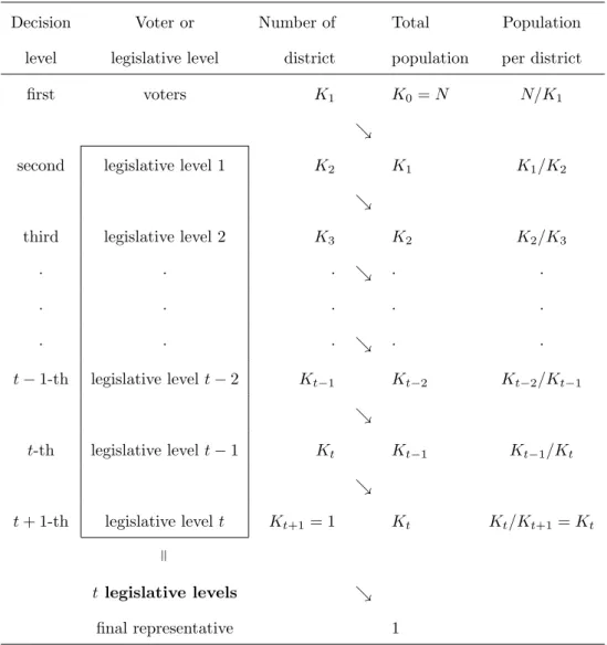
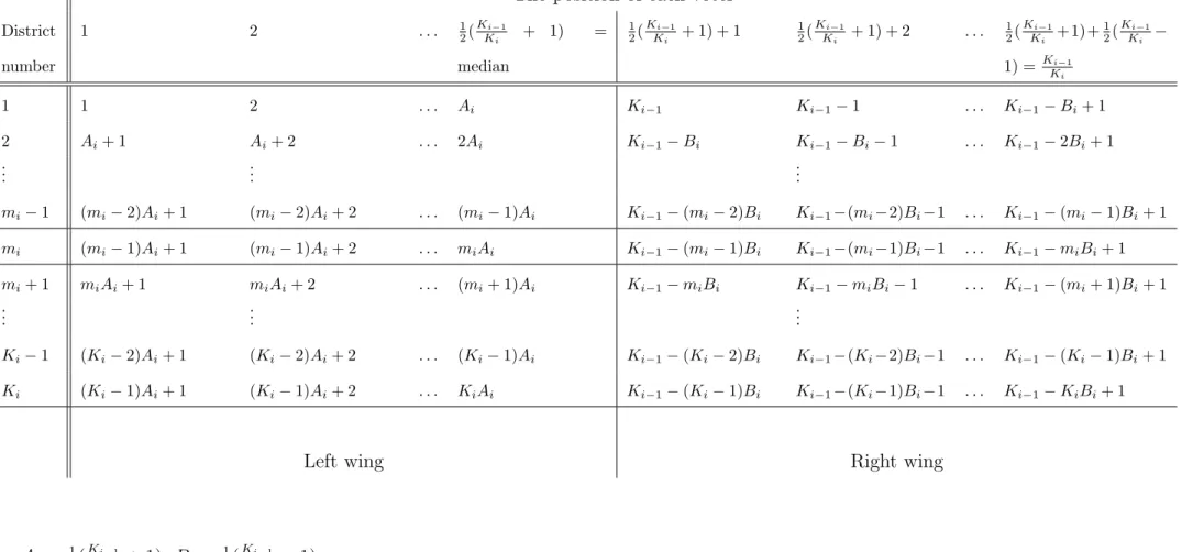
We considert+ 1 decision levels, starting fromt= 0. At decision level i∈ {1,2, . . . , t−1, t}, voters grouped into equally sized districts send a representative to a legislature at thei+ 1-th decision level. Let Ki be the number of districts at the i-th decision level. In order to finally elect a single representative who decides on a policy, only one district is formed at the t+ 1-th decision level. Thus, we let Kt+1 = 1. For convenience, let K0 =N.
Assumption 1. N is odd and the district size Ki−1/Ki at level i is an odd integer for any i∈ {1, . . . , t+ 1}.
If not stated otherwise, we assume that Assumption 1 holds.5
When t= 0, there are no legislatures between voters and the final representative. Only one representative, who implements a policy, is elected directly from among the voters. We view this as a direct democracy. When t ≥ 1, our model becomes an indirect democratic system and, especially when t ≥ 2, has hierarchical legislatures with multiple levels. We assume that every voter and representative at each i-th decision level casts a ballot sincerely and that only one among them is elected as a single-member district representative by a majority rule.
4In Gilligan and Matsusaka, the cumulative distribution function F(x∗P OP) = 1/2 at the median’s ideal policy is defined. However, this definition is not appropriate because the authors assume discrete voters andN is odd. For example,N = 27,F(x∗pop) = 14/276= 1/2.
5Nevertheless, in the statements of our lemmas, propositions, and corollaries, we explicitly require Assump- tion 1 whenever needed.
Accordingly, the median voter of each district is elected as the representative, and every district at thei+ 1-th decision level is composed of the median voters from each district at next lower level. Thus, Ki is also the number of representatives at the i+ 1-th decision level. From the assumption of equally sized districts at the same level, the population of each district at the i+ 1-th decision level isKi/Ki+1. Naturally, we must haveKi+1 < Ki, since we elect fewer and fewer representatives as we move upwards in the hierarchy.
In summary, the basic structure of our model is as follows. First, N voters are divided into K1equal-sized districts. Then,N/K1 =K0/K1voters per district at the first decision level elect the representatives of legislative level 1 at the second decision level. Consequently, legislative level 1 comprises K1 representatives. Second, the representatives of legislative level 1 are divided into K2 equal-sized districts andK1/K2 members per district elect the representatives of legislative level 2 at the third decision level. Consequently, legislative level 2 comprises K2
representatives. Third, the representatives of legislative level 2 are divided into K3 equal-sized districts and K2/K3 members per district elect the representatives of legislative level 3 at the fourth decision level. Consequently, legislative level 3 comprisesK3 representatives, and so on.
Finally, since the t+ 1-th decision level is the final level and Kt+1 = 1, the Kt representatives of legislative level t at the t+ 1-th decision level elect only one representative, who is the final representative. Thus,tdenotes the number of hierarchical legislative levels inserted between the voters and the final representative. These levels are, for example, ward representatives, county representatives, state representatives, and national representatives. The final representative decides and implements only one policy, which is a number on the real line, that applies to all voters. Table 1 depicts the above structure. Here, we assume that neither voters nor representatives can commit to policies. Thus, the final representative implements his/her own ideal policy. Note that Gilligan and Matsusaka’s model is a special case of our model, where t = 1. Additionally, there is no vote-value disparity because of the equal-size districts at each level.
From the above structure, we can immediately obtain the following lemma:
Lemma 1. Under Assumption 1, the number of hierarchical levels is at most the number of
Table 1: The basic structure of the model
Decision Voter or Number of Total Population
level legislative level district population per district
first voters K1 K0=N N/K1
&
second legislative level 1 K2 K1 K1/K2
&
third legislative level 2 K3 K2 K2/K3
· · · & · ·
· · · · ·
· · · & · ·
t−1-th legislative levelt−2 Kt−1 Kt−2 Kt−2/Kt−1
&
t-th legislative levelt−1 Kt Kt−1 Kt−1/Kt
&
t+ 1-th legislative levelt Kt+1= 1 Kt Kt/Kt+1=Kt
=
t legislative levels &
final representative 1
prime factors of N.
Proof. We prove this by contradiction. Let N = a1 ·a2 ·a3· · ·at·at+1, where each ai, i ∈ {1,2,3, . . . , t, t+ 1}, is a prime factor of N. We assume that for given N we can make j + 1 decision levels, noting Ki > Ki+1 and Kj+1 = 1, where j > t. Then, the populations of each district at each level 1,2,3, . . . , j, j+ 1 are KN
1,KK1
2,KK2
3, . . . ,KKt−1
t , . . . ,KKj
j+1, respectively. Thus, N = N
K1 ·K1 K2 · K2
K3 . . .Kt−1
Kt . . . Kj Kj+1,
and the number of the factors of N is j+ 1. However, N cannot be the product of more than t integers larger than 1 from its prime factorization, which is a contradiction.
Hereafter, for convenience, t∗ + 1 is regarded as the maximum number of decision levels (under Assumption 1) and the number of the prime factors of N. Note that we can set up
hierarchical decision levels between 0 and t∗+ 1 by multiplying together any prime factors of N. For instance, supposeN = KN
1 ·KK1
2 ·KK2
3 . . .KKt∗
t∗+1. We can also set up t∗−1 decision levels in addition tot∗+ 1 levels if we multiply the first three prime factors, KN
1·KK1
2·KK2
3, with populations per district of KN
3,KK3
4, . . . ,KKt∗
t∗+1 at each decision level, respectively. See also Example 1.6 Letx∗i,k be the ideal point andji,k∗ be the index (i.e.,xj∗
i,k =x∗i,k) of the median representative or voter in districtk at thei-th decision level (i.e., legislative leveli−1). When there aret+ 1 decision levels, at the final decision level, where Kt+1 = 1, the policy outcome decided in the final legislative level becomes x∗t+1,1.
How do liberal voters gerrymander to maximize their own political payoff? We shall assume that a liberal extremist, called voter 1, can arrange all districts.7 Then, this person will attempt to put a representative who is as left as possible on the median position in each district at each decision level. We can say that the more to the left the final representative falls, the stronger is her policy implementability. In this paper, we use the well-known “cracking and packing”
algorithm at each decision level, as formulated by Gilligan and Matsusaka. They describe the algorithm as follows.
“First, citizens with high-value ideal points are “cracked” into districts where they are the minority, maximizing the influence of citizens with low-value ideal points, and second, the remaining high-value citizens are “packed” into districts contain- ing a preponderance of like-minded citizens in order to waste their votes through overkill.”
In the next example, we specifically show how far away the final policy in the multiple hierarchical electoral system under the extremist’s gerrymandering can be from the policy
6 It might look as though Lemma 1 imposes a severe restriction on the number of possible decision levels.
For instance, ifN is a prime number, we can construct only one district at the first decision level because of the assumption of equal-sized districts. We can overcome this problem by changing “equal-sized districts” slightly to “almost equal-sized districts” by roundingKi/Ki+1either up or down. Then, we consistently pick one of the two electors from “the middle” in the case of even district sizes. However, this extension would just complicate our analysis and would produce the same results. See also Example 2.
7Of course, in the same way, we can also consider a conservative extremist instead of a liberal extremist.
decided in a direct democracy (i.e., the median voter’s ideal policy). We compare the final policy in our model with the policy in the model of Gilligan and Matsusaka in the next example.
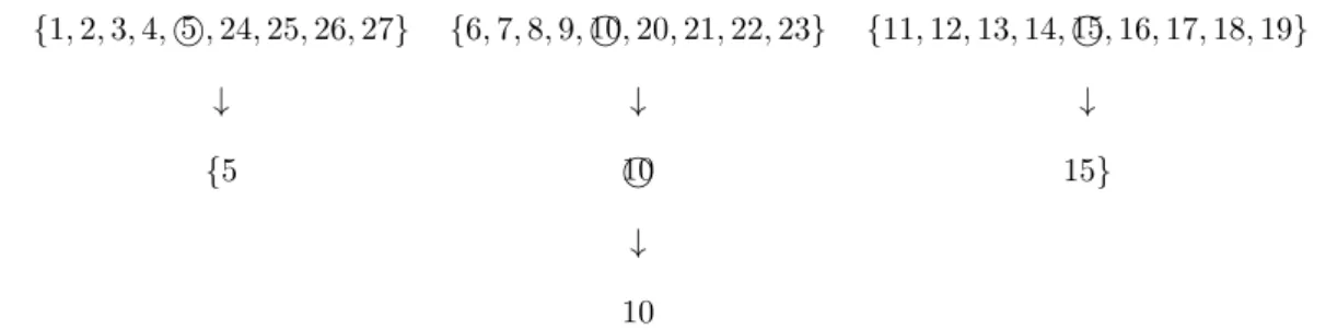
Example 1. We consider an example of three decision levels, where t+ 1 = 3, N = 27, voters set N = {1,2,3, . . . ,25,26,27}, and voters have ideal points at xj = j. We compare the indirect democracies of two decision levels (t = 1) and three decision levels (t = 2) with the direct democracy (t = 0).8 In this case, the median voter is N+12 = 14, as shown in Table 2, so that the final policy is decided at x∗1,1 = x14 in the direct democracy. However, as shown
Table 2: The case of N = 27, K1 = 1
{1,2,3,4,5,6,7,8,9,10,11,12,13,14,15,16,17,18,19,20,21,22,23,24,25,26,27}
↓ 14
by Gilligan and Matsusaka, the final policy is not always decided at the median of all voters in an indirect democracy with gerrymandered districts. Here, we show that the selected policy becomes further from the median as the levels increase. Table 3 and Table 4 illustrate the most extreme gerrymandering to give an advantage to liberal (left) voters in the case of two decision levels (t = 1). These can be regarded as regular indirect democracies, where the final representative is elected from the legislature composed of the representatives elected in single-member districts.
For t= 1 and N = 27, we can consider two cases where (K1, K2) = (3,1) and (9,1). Then, we can easily find the final representative who is as close as possible to voter 1, who is a liberal extremist, as in the example with nine voters in Gilligan and Matsusaka. In both Tables 3 and 4, the policies are decided by voter 10, whose ideal position is 4 positions away from the
8Here, 27 is equal to 3·3·3 by the prime factor decomposition. From this fact, in the case of two decision levels, each district at the first decision level and at the second level are composed of 9 voters and 3 representatives, respectively, or of 3 and 9, respectively. In the case of three decision levels, each district is composed of three voters or representatives at every decision level. As a result, we can obtain combinations of K1 = 1, (K1, K2) = (3,1),(9,1), and (K1, K2, K3) = (9,3,1) for the cases of one decision level, two decision levels, and three decision levels, respectively.
Table 3: The case of N = 27,K1 = 3, K2 = 1
{1,2,3,4,,5 24,25,26,27} {6,7,8,9,10,20,21,22,23} {11,12,13,14,15,16,17,18,19}
↓ ↓ ↓
{5 10 15}
↓ 10
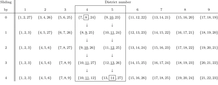
Table 4: The case of N = 27,K1 = 9, K2 = 1
{1,,2 27} {3,,26}4 {5,,25}6 {7,,8 24} {9,10,23} {11,12,22} {13,14,21} {15,16,20} {17,18,19}
↓ ↓ ↓ ↓ ↓ ↓ ↓ ↓ ↓
{2 4 6 8 10 12 14 16 18}
↓ 10
median voter. Even if there are several district patterns in a combination of N and t, it can be shown that the maximum distances between the final representative and the median are identical in the case of optimal gerrymandering for either the liberal or conservative extremists who are “partisan.”
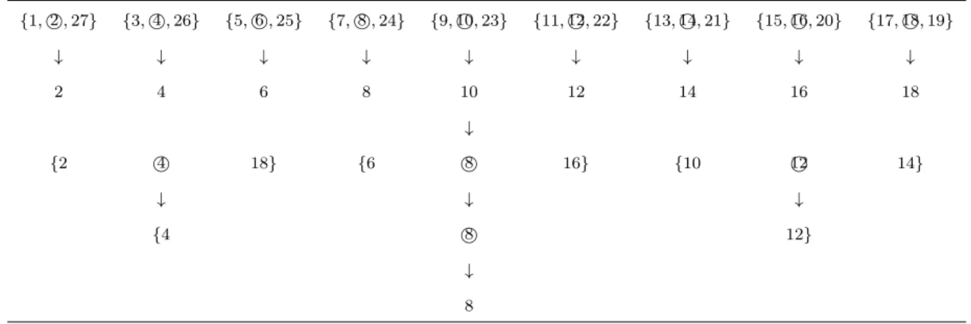
Finally, what is the policy decided by the upper representatives if an additional level of representation is incorporated in the above decision process in the case of gerrymandering? In the same way as in our previous examples with two decision levels, the districts at the second decision level are arranged by one liberal extremist in order to implement a final policy as close as possible to her own ideal point. In the case of three decision levels, the districts pattern is only (K1, K2, K3) = (9,3,1). Table 5 illustrates this case. The policy is decided by voter 8, who is 6 positions away from the median. This is even further from the median than in the case of two decision levels. This example suggests that the final policy decided in the gerrymandered districts becomes further from the median as we add more hierarchical decision levels to the democratic representative system. We revisit this fact in Proposition 1 in the next section. Additionally, from the result of Lemma 1, many voters are required to construct a higher hierarchical representative system.
Table 5: The case of N = 27, K1 = 9, K2 = 3, K3 = 1
{1,,2 27} {3,,26}4 {5,,25}6 {7,,8 24} {9,10,23} {11,12,22} {13,14,21} {15,16,20} {17,18,19}
↓ ↓ ↓ ↓ ↓ ↓ ↓ ↓ ↓
2 4 6 8 10 12 14 16 18
↓
{2 4 18} {6 8 16} {10 12 14}
↓ ↓ ↓
{4 8 12}
↓ 8
Actually, in Example 1, where N = 27, the liberal extremist can only construct at most three decision levels if we require strictly equal-sized districts and odd district sizes. We already mentioned in footnote 6 that Lemma 1 is not as restrictive as it might first appear. To see this we provide another example withN = 27 voters.
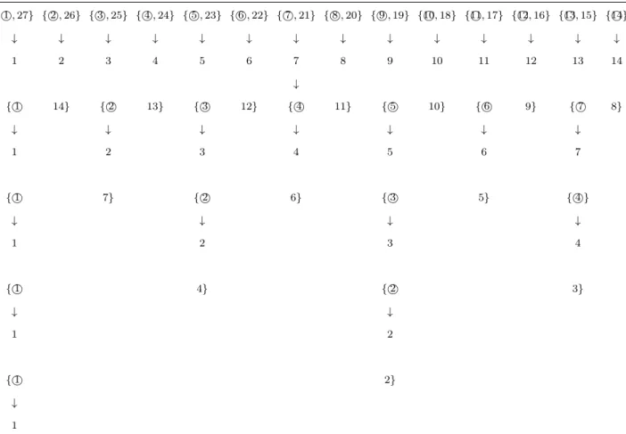
Example 2. LetN = 27 and the target district size be 2, which means that districts contain either 1 or 2 voters. Clearly, if we put just one voter in a district, she will be the winner of her district. If we put two voters in a district, the median voter is not uniquely defined. In this example, we assume that the left of the two voters in the middle will be elected. 9 Table 6 illustrates this case.
We make two observations based on Example 2. First, for a given N, we can have more biased outcomes in the case of indivisibilities and even-numbered district sizes. This statement will become clearer after the discussion of Lemma 2. Second, once almost-equal-sized districts and even-numbered district sizes are allowed, while neither is allowed in Lemma 1, the maximum number of levels monotonically increases as the number of voters increases. In particular, if at the i-th decision level, Ki−1 is not divisible by Ki, then there exists a unique positive integer si and integer 0 ≤ ri < Ki such that Ki−1 = siKi −ri. Then, we have si = dKi−1/Kie, and we can form Ki−ri districts of size si and ri districts of size si−1. Clearly, we can obtain a maximum number of decision levels by taking sequence Ki =N −i as the number of districts
9Clearly, one could choose the right-hand voter or determine the winner randomly. In the latter case, the most extreme outcome would be if, at each level and each district, the left or right voter was always chosen.
Table 6: The case of N = 27, K1 = 14, K2 = 7, K3 = 4, K4 = 2, K5 = 1
{,1 27} {,26} {2 ,25} {3 ,4 24} {,5 23} {,22} {6 ,7 21} {,8 20} {,19} {109 ,18} {11,17} {12,16} {13,15} {14}
↓ ↓ ↓ ↓ ↓ ↓ ↓ ↓ ↓ ↓ ↓ ↓ ↓ ↓
1 2 3 4 5 6 7 8 9 10 11 12 13 14
↓
{1 14} {2 13} {3 12} {4 11} {5 10} {6 9} {7 8}
↓ ↓ ↓ ↓ ↓ ↓ ↓
1 2 3 4 5 6 7
{1 7} {2 6} {3 5} {}4
↓ ↓ ↓ ↓
1 2 3 4
{1 4} {2 3}
↓ ↓
1 2
{1 2}
↓ 1
at leveli. In this case, the number of decision levels is equal to the number of voters.
A more natural way to generate a sequenceK0, K1, . . . , Kt, Kt+1 would be to fix a sequence s1, s2, . . . , st of target district sizes. This means we have either si or si−1 representatives in each district at decision level i, the number of districts Ki at decision level i is determined by Ki−1 = siKi −ri, where 0 ≤ ri < Ki and si = dKi−1/Kie, and we have Ki −ri districts of size si and ri districts of size si −1. Of course, not every sequence s1, s2, . . . , st of positive integers is admissible. It would make sense to look for sequences that remain constant as long as possible (i.e.,s =s1 =s2 =. . .=sq for a q≤t as large as possible), since then the number of representatives decreases at the same rate as we move upwards in the hierarchy. If choosing s as the target size for each decision level is possible, then the number of hierarchical decision levels is given bydlogsNein the function ofN. Hence, as the number of voters tends to infinity, the number of decision levels also tends to infinity.
Finally, we investigate whether si is a valid target value for the number of representatives
at decision level i. Since ri has to satisfy 0 ≤ri < Ki, we obtain 0 ≤siKi−Ki−1 < Ki, which in turn implies
Ki−1
si ≤Ki < Ki−1
si−1. (1)
A sufficient condition for the existence of an integer Ki satisfying (1) is Ki−1
si−1 −Ki−1
si ≥1 ⇐⇒ si(si−1)≤Ki−1. (2) Since si(si−1) < s2i, a sufficient condition for the existence of an integer Ki satisfying (1) is given by
si ≤p
Ki−1. (3)
Assuming that we are striving for a constant sequence s = s1 = s2 = . . . = st, then the violation of condition (3) means that adding two more levels with target district sizess would be impossible. Therefore, for the top two levels, the target district size s has to be reduced appropriately and, at the same time, we can still achieve at least dlogsNe decision levels.
3 Extremists’ policy implementability
From Example 1, we can conjecture that the final elected voter is getting further from the median of all voters as we add more hierarchical levels of legislatures, when all districts at each level are arranged by a liberal extremist’s gerrymandering. The following lemma determines the final elected voter’s position in the t+ 1 decision levels, composed of both voters and t hierarchical legislative levels in the indirect democracy. Note that, by Lemma 1, there are at most t∗+ 1 decision levels in the case of N voters and that the number of decision levels lies between 0 and t∗+ 1. Then, the final elected voter’s position is shown in the next lemma.
Lemma 2. (Generalization of Gilligan and Matsusaka (2006)) If Assumption 1 is sat- isfied, then in the case of liberal gerrymandering, the policy outcome is decided by voter
jt+1,1∗ = 1 2
1 2
t
1
KtKt−1· · ·K2K1(Kt+ 1)(Kt+Kt−1)(Kt−1+Kt−2)· · ·(K2+K1)(K1+N) (4) in the political decision system composed of t+ 1 (t ∈ {0,1,2, . . . , t∗}) hierarchical decision levels.
Proof. We prove formula (4) by backward induction. First, the final representative (she) is elected at the t+ 1-th decision level. Given thatKt+1 = 1, for her final win, she needs at least a minimum majority: that is, 12
Kt
Kt+1 + 1
= 12(Kt+ 1) representatives with smaller numbers than hers and herself at the t+ 1-th decision level.
Second, since each representative at the t+ 1-th decision level is elected in each district at the t-th decision level, to win a majority at t+ 1-th decision level, she needs at least 12(Kt+ 1) districts, including 12
Kt−1
Kt + 1
representatives with smaller numbers than hers per district and herself at thet-th decision level. Consequently, she needs 12
Kt−1
Kt + 1 1
2(Kt+1) representatives with smaller numbers than hers and herself at the t-th decision level.
Third, given that each representative at the t-th decision level is elected in each district at thet−1-th level, for the final representative to win with 12
Kt−1
Kt + 1 1
2(Kt+ 1) representatives supporting her at the t-th decision level, she needs at least 12
Kt−1
Kt + 1 1
2(Kt+ 1) districts, including 12(KKt−2
t−1+ 1) representatives with smaller numbers than hers and herself per district at thet−1-th level. Consequently, she needs 12(KKt−2
t−1+ 1)12(KKt−1
t + 1)12(Kt+ 1) representatives with smaller numbers than hers and herself at the t−1-th decision level. The same logic continues until we reach the voters level.
Finally, at voters level (i.e, the first level), she needs at least 1
2 K0
K1 + 1 1
2 K1
K2 + 1
. . .1 2
Kt−2
Kt−1
+ 1 1
2
Kt−1
Kt + 1 1
2(Kt+ 1) (5) representatives with smaller numbers than hers and herself. This formula is equal to (4). Hence the position of the final representative with the smallest number is (4).
Lemma 2 includes the case of the most extremely liberal gerrymandering with t+ 1 decision levels. By symmetry of voters, we can easily obtain the position N −jt+1,1∗ + 1 by the most extremely conservative gerrymandering. Additionally, (4) also indicates the representative po- sition in the direct democracy at t= 0. Thus, the direct democracy can be viewed as a special case of this hierarchical legislature.
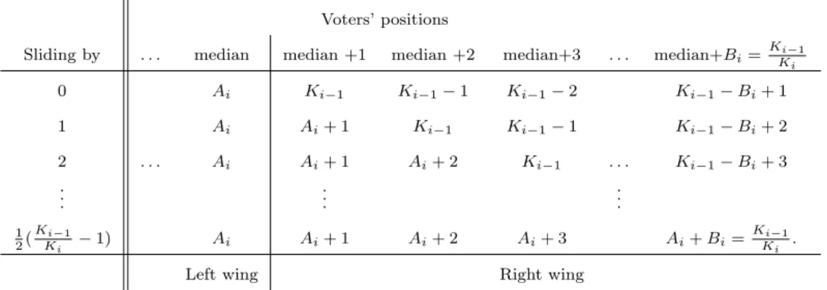
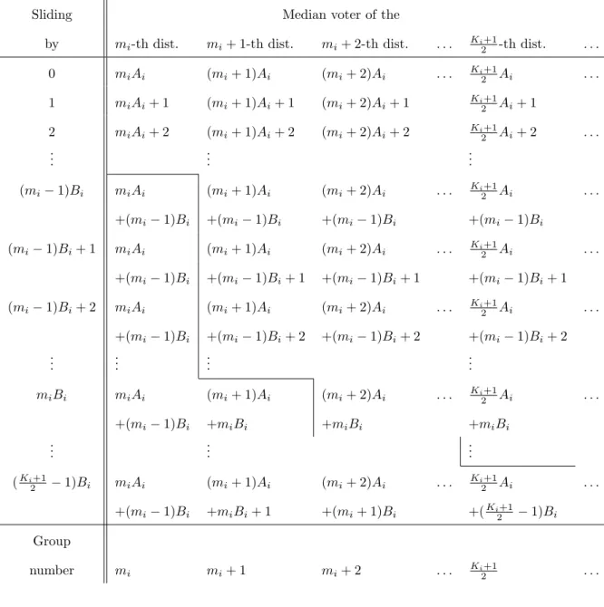
Focusing on (5), in the most extremely liberal gerrymandering with t+ 1 decision levels, the final elected voter’s position is determined by constructing districts as nested boxes, with
they have the decision power. In other words, voters with higher values than hers have no influence in this gerrymandering. Thus, the result does not depend on the order of packing voters into districts.
Example 2 already explained how we can get rid of our assumptions of equal- and odd-sized districts (i.e., Assumption 1). Now, we explain how to obtain an upper bound on the most leftward voter deciding the policy outcome, based on Lemma 2, if we also allow for almost equal and even-sized districts, as described in Example 2.
Lemma 3. In the case of liberal gerrymandering, we have the following upper bound on the voter deciding the policy outcome:
jt+1,1∗ ≤ 1 2
1 2
t
1
KtKt−1· · ·K2K1(Kt+ 1)(Kt+Kt−1)(Kt−1+Kt−2)· · ·(K2+K1)(K1+N) (6) in the political decision system composed of t+ 1 hierarchical decision levels.10
Proof. In order to obtain an upper bound for jt+1,1∗ for the more general case, we just have to follow the steps of the proof of Lemma 2. First, if Kt is even, the final representative needs at least a minimum majority: that is, 12Kt representatives with smaller numbers than hers and herself at the t+ 1-th decision level, which is less than the 12(Kt+ 1) obtained for the odd-size case. Second, since each representative at thet+ 1-th decision level is elected in each district at the t-th decision level, to win a majority at the t+ 1-th decision level, she needs at least either 12Kt or 12(Kt+ 1) districts, including either 12KKt−1
t representatives from each of the even-sized districts, or 12
Kt−1
Kt + 1
representatives from each of the odd-sized districts with smaller numbers than hers per district and herself at thet-th decision level. Consequently, she does not need more than 12
Kt−1
Kt + 1
1
2(Kt+ 1) representatives with smaller numbers than hers and herself at the t-th decision level. By analogous modifications in the remaining steps
10Note that the indexes ji,k∗ can be extended in an obvious way to the case in which Assumption 1 does not hold. More precisely, if an even district size emerges at level i in district k in our electoral system, then the actual value ofji,k∗ depends on how we choose between the two voters in the “middle.” Here, and in what follows, we assume in the extension ofj∗i,kthat the left of the two representatives in the middle will be elected to the next higher level, since this results in the most biased outcome. For more on this, we refer to the discussion after Example 2.
of the proof of Lemma 2, we find that the right-hand side of (4) provides an upper bound on jt+1,1∗ for the general case.
Formula (4) is obtained as the representative with the policy that is implementable and nearest to the liberal extremist’s ideal policy for given t+ 1 decision levels and N. As a conse- quence of the formula, the next proposition states the monotonic decrease of the representative’s position ast increases for given N.
Proposition 1. Under Assumption 1, for given N, the final representative position is moving further from the median of voters monotonically as the number of hierarchical stages increases.
Proof. Let N =a1 ·a2 ·a3. . .·at∗·at∗+1, where all of ai, (i = 1, . . . , t∗+ 1) are prime factors of N. From Lemma 1, N = KN
1 · KK1
2 · KK2
3 ·. . .· KKt∗−1
t∗ · KKt∗
t∗+1, noting that Kt∗+1 = 1 in the case of the maximum number of hierarchical levels, t∗+ 1. Without loss of generality, we let
N K1,KK1
2,KK2
3, . . . ,KKt∗−1
t∗ ,KKt∗
t∗+1 equal a1, a2, a3, . . . , at∗, at∗+1, respectively. Then, we obtain K1 =
N
a1,K2 = aN
1a2, K3 = a N
1a2a3, . . .,Kt∗ = a N
1a2a3...at∗, Kt∗+1 = a N
1a2a3...at∗at∗+1 = 1.
In the case in which there are t+ 1 (t = 1, . . . , t∗) decision levels, N = b1b2. . . bt+1, where each bi (i = 1, . . . , t) is a product of some prime factors of N. Using the same method, we obtain K1 = Nb
1, K2 = bN
1b2, K3 = b N
1b2b3, . . ., Kt = b N
1b2b3...bt, Kt+1 = b N
1b2b3...btbt+1 = 1. Here, when the number of total levels is t, we choose any two factors in {b1, b2, . . . , bt+1}and find the product. For simplicity, we choose the last two factors,btbt+1. Then, we getK1 = Nb
1,K2 = bN
1b2, K3 = b N
1b2b3, . . ., Kt−1 = b N
1b2b3...bt−1, Kt0 = b N
1b2b3...btbt+1 = 1. Comparing the case of t levels with the case oft+ 1 levels, each ofK1 through Kt−1 is identical.
We calculate the ratio of jt,1∗ and jt+1,1∗ : jt,1∗
jt+1,1∗ =
1 2
1 2
t−1 1
Kt−1Kt−2···K2K1(Kt−1 + 1)(Kt−1+Kt−2)(Kt−2+Kt−3)· · ·(K2+K1)(K1+N)
1 2
1 2
t 1
KtKt−1···K2K1(Kt+ 1)(Kt+Kt−1)(Kt−1+Kt−2)· · ·(K2+K1)(K1+N)
= Kt−1+ 1
1 2
1
Kt(Kt+ 1)(Kt+Kt−1)
= 2Kt(Kt−1+ 1) (Kt+ 1)(Kt+Kt−1).
Here, since ∀t ∈ {1,2,3, . . . , t∗}, Kt−1 > Kt > 1, and 2Kt(Kt−1 + 1)−(Kt+ 1)(Kt+Kt−1) = (Kt−1)(Kt−1 −Kt) > 0, the numerator is larger than the denominator. Thus, jt,1∗ > jt+1,1∗ ,
By this proposition, we can say that a voter with a policy position nearer to the extremist’s ideal policy becomes electable as the decision levels get higher for given N. In other words, the hierarchical legislative system with more levels increases the policy implementability of the extremist.
For given numbers of voters N and levels t, we can determine the number of districts K1, . . . , Kt that results in the most biased outcome that is the furthest representative position from the median. Noting that K0 =N, the next proposition can be obtained.
Proposition 2. If Assumption 1 is satisfied, then in the case of N voters and t+ 1 decision levels for which t+1√
N is an integer, the multi-level districting given by
∀i= 1, . . . , t, t+ 1 :Ki =Nt−(i−1)t+1 (7) admits the largest possible bias.
Proof. Determining the maximum bias is equivalent to minimizing jt+1,1∗ /N with respect to K1, . . . , Kt. Noting thatN =K0,
jt+1,1∗
N =
1 2
t+1
1
KtKt−1· · ·K2K1K0
(Kt+ 1)(Kt+Kt−1)(Kt−1+Kt−2)· · ·(K2+K1)(K1+K0), we multiply 1/K0,1/K1, . . . ,1/Ktby the terms in the previous formula in reverse order. Hence, we have to minimize the expression
1 2
t+1 1 + 1
Kt 1 + Kt Kt−1
· · ·
1 + K2
K1 1 + K1 K0
, (8)
yielding first-order conditions equivalent to 0 =−Ki+1
Ki2
1 + Ki Ki−1
+
1 + Ki+1 Ki
1 Ki−1
,
for all i= 1, . . . , t. Thus, by simple rearrangements, we obtain
Ki+1Ki−1 =Ki2, (9)
for all i= 1, . . . , t, where Kt+1 = 1. It can be verified that the first-order conditions determine the minimum value for expression (8).
We claim that
Kt−(i−1) = (Kt−i)i+1i , (10)
for all i = 1, . . . , t, which we prove by induction. Clearly, our claim holds true for i = 1, by equation (9). Assume that (10) is valid for i. Therefore, we show that it also holds true for i+ 1. From (9), we have
Kt−i+1Kt−i−1 = (Kt−i)2, and by employing our induction hypothesis, we get
(Kt−i)i+1i Kt−i−1 = (Kt−i)2 ⇔ Kt−i = (Kt−i−1)i+1i+2 , which is what we wanted to show.
Finally, by employing (10) recursively, we obtain the statement of our proposition.
Assuming in Proposition 2 that t+1√
N is an integer may appear to be too restrictive.11 Clearly, for arbitrary combinations of N and t, the sequence (Ki)t+1i=1 given by equation (7) is typically a non-integer sequence and does not determine legitimate numbers of districts for all levels. However, we only use the result of Proposition 2 to get an idea of how to find a lower bound for the largest possible bias while keepingt fixed.
Proposition 3. If the number of levels t is fixed, then as the number of voters N tends to infinity, we have the following lower bound on the bias of the most biased case:
Nlim→∞max
F(x∗t+1,1)−F(x∗P OP) ≥ 1
2− 1
2 t+1
.
Proof. Noting that lim
N→+∞F(x∗P OP) = 1/2, from Lemma 3, we get
Nlim→∞maxB(x) = 1
2 −jt+1,1∗
N ≥ 1
2 −
1 2
K0
K1 + 1
1 2
K1
K2 + 1
· · ·12
Kt−1
Kt + 1
1
2(Kt+ 1)
K0
K1
K1
K2 · · ·KKt−1
t
Kt
Kt+1
= 1
2 −1 2
1 + K1 K0
1 2
1 + K2 K1
· · ·1 2
1 + Kt Kt−1
1
2(1 +Kt). (11) Now, in the hierarchical construction described in Example 2, we substitute bt+1√
Nc for the target district size s. Since we are only interested in the case of many voters, we can assume,
11Not to mention, if all prime factors ofN are identical, for example,N =at+1, whereais a prime, t+1√ N is
without loss of generality, that blogsNc −1 ≥ t. It can be verified that for fixed t, for the determined value ofs, and for sufficiently largeN, a sequenceK1, . . . , Ktof numbers of districts can be chosen in the way described at the end of Example 2. Hence, substituting the target district sizes into (11), we obtain
lim
N→∞maxB(x)≥ lim
N→∞
1 2 −
1 2
t+1 1 + 1
s 1 + 1 s
· · ·
1 + 1 s
= 1 2−
1 2
t+1
,
since s tends to infinity as N tends to infinity for a given t.
Noting that (8) is not jt+1,1∗ , but rather jt+1,1∗ /N, which is the relative position of the final elected voter, this proposition says that the relative position of the voter moves left as N increases. Now, from Proposition 3, it follows that as the maximum number of levels t increases, the maximum bias approaches its highest possible level, which we state in the next corollary.
Corollary 1. As t tends to infinity, the maximum bias in the case of liberal gerrymandering tends to 1/2.
Proposition 3 and Corollary 1 mean that the more voters there are, the more extreme the relative position of the policy that political extremists can realize becomes. As a result, many voters provides the extreme district maker with an expedient way to implement her favorite policy. In particular, if party A is at the left end and party B is at the right end of the unit interval, then, party A’s most preferred outcome will be the national outcome, independent of voters’ preferences.
Our model is applicable to other democratic issues. In the Appendix, we apply our model to solve and explain the issues of random districting and the partisan bias.
4 Moderates’ policy implementability
So far, we have only considered the cracking and packing method in the case in which a political extremist is a district maker who wants to implement a policy as low or as high as possible.
However, someone with a moderate political position around the median can also be a district