Robust estimation in time series with long and short memory properties

Robust estimation in time series with long and short memory properties

Valdério Anselmo Reisen, Fabio Fajardo Molinares

Departamento de Estatística, Universidade Federal do Espírito Santo, Vitória/ES, Brazil valderioanselmoreisen@gmail.com,fabio.molinares@ufes.br.

Dedicated to Mátyás Arató on his eightieth birthday

Abstract

This paper reviews recent developments of robust estimation in linear time series models, with short and long memory correlation structures, in the presence of additive outliers. Based on the manuscripts Fajardo, Reisen &

Cribari-Neto 2009 [7] and Lévy-Leduc, Boistard, Moulines, Taqqu & Reisen 2011 [19], the emphasis in this paper is given in the following directions; the influence of additive outliers in the estimation of a time series, the asymptotic properties of a robust autocovariance function and a robust semiparametric estimation method of the fractional parameterdin ARFIMA(p, d, q)models.

Some simulations are used to support the use of the robust method when a time series has additive outliers. The invariance property of the estimators for the first difference in ARFIMA model with outliers is also discussed. In general, the robust long-memory estimator leads to be outlier resistent and is invariant to first differencing.

Keywords: Additive outliers, ARFIMA model, long-memory, robustness.

1. Introduction

Let{Xt}^t∈Z be a stationary time series with spectral density that behaves like fX(ω)∼h(ω)|ω|^−2d, as ω→0 (1.1) where the spectral densityh(ω)is a nonvanishing and continuously differentiable function with bounded derivative for−π≤ω≤π, andd <0.5.

A well-known stationary parametric model with the above spectral density is the ARFIMA(p, d, q)process, which is the solution of the equation

Xt−µ= (1−B)^−dηt, t∈Z, (1.2)

Proceedings of the Conference on Stochastic Models and their Applications Faculty of Informatics, University of Debrecen, Debrecen, Hungary, August 22–24, 2011

207

whereηt= ^Θ(B)_Φ(B)tis an ARMA(p, q)process,µis the mean (here it is assumed that µ= 0), Φ(B)≡1−Pp

j=1φjB^j,Θ(B)≡1−Pq

i=1θiBⁱ and pandq are positive integers (Hosking 1981 [11]). Φ(z)andΘ(z), with a scalarz, are the autoregressive and moving average polynomials with all roots outside the unit circle and share no common factors. d is the parameter that holds the memory of the process, that is, whend∈(−0.5,0.5) the ARFIMA(p, d, q)process is said to be invertible and stationary. Besides, ford6= 0, its autocovariance decays at a hyperbolic rate (γ(j) = O(j^−1+2d)). For d = 0, d ∈ (−0.5,0) or d ∈ (0,0.5), the process is said to be short-memory, intermediate-memory or long-memory, respectively. The long-memory property is related to the behavior of the autocovariances, which are not absolutely summable and the spectral density becomes unbounded at zero frequency. In the intermediate-memory region, the autocovariances are absolutely summable and, consequently, the spectral density is bounded.

The spectral density function of {Xt}^t∈Z is given by fX(ω) =fη(ω)h

2 sinω 2

i−2d

, ω∈[−π, π]. (1.3) fX(ω) is continuous except forω = 0where it has a pole when d > 0. A recent review of the ARFIMA model and its properties can be found in Palma 2007 [23]

and Doukhan, Oppenheim & Taqqu 2003 [6].

Many estimators for the fractional parameterdin long-memory time series have already been proposed in the literature. Among them are the semiparametric pro- cedures, a group which includes a wide variety of estimators based on the Ordinary Least Square (OLS) method. These procedures require the use of the spectral den- sity parameterized within a neighborhood of zero frequency. Some references on this subject include the works of Geweke & Porter-Hudak 1983 [10], Reisen 1994 [26] and Robinson 1995 [27], among others. An overview of long-range dependence processes can be found in Beran 1994 [1] and Doukhan et al. 2003 [6].

Time series with outliers or atypical observations is quite common in any area of application. In the case where the data is time-dependent, several authors such as Ledolter 1989 [17], Chang, Tiao & Chen 1988 [4] and Chen & Liu 1993 [5] have studied the effect of outliers in a time series that follows ARIMA models. In general, they have concluded that the parameter estimates of ARMA models become more biased when the data contains outliers. Similar conclusion is also observed when estimating the fractional parameter in ARFIMA models. The outliers cause a substantial bias in the differencing parameter (Fajardo et al. 2009 [7]).

An autocovariance robust function was proposed by Ma & Genton 2000 [20].

The asymptotical properties of this function are studied by Lévy-Leduc et al. 2011 [19]. The results presented in Fajardo et al. 2009 [7], Lévy-Leduc et al. 2011 [19]

and Lévy-Leduc, Boistard, Moulines, Taqqu & Reisen 2011 [18] are the motivations of this paper. The impact of outliers in the estimation of ARFIMA models under different context is here studied. The asymptotical properties of a robust autoco- variance function is discussed and some empirical examples are used to illustrate the usefulness of a robust fractional parameter estimator. The invariance property

of the estimator to the first difference is also empirically studied. The outline of this papers is as follows: Section 2 discusses the model and the impact of the outliers in time series. Section 3 summarizes the main results related to the robust auto- covariance estimator given in Lévy-Leduc et al. 2011 [19] and discusses the robust estimation of the fractional parameter in the ARFIMA model. Section 4 presents some empirical studies and an application is discussed in Section 5. Concluding remarks and future directions are given in Section 6.

2. The impact of outliers in time series

Suppose x1, ..., xn is a partial realization of {Xt}^t∈Z. Hence, the periodogram function is defined asIx(ω) = (2πn)⁻¹|Pn

t=1xte^iωt|². It follows that, whend= 0 in the ARFIMA model,

Ix(ω) = 2πfX(ω)I(ω)

σ² +H(ω) (2.1)

where E[|H(ω)|²] =O(_n¹2ξ)(ξ >0) is uniformly inω ∈[−π, π] (Theorem 6.2.2 in Priestley 1981 [25]) andI(·)is the periodogram of the residuals. From (1.2) and Theorem 6.1.1 in Priestley 1981 [25], asymptotic sample properties of _f^I_X^x(ω)_(ω) are derived and they are summarized as follows. If{t}t∈Z are normally distributed, for a fixed set of values of the Fourier frequenciesωj= ^2πj_n ,j= 1, ...,[n/2], where[·] means the integer part, asymptotically the set of variables _f^I_X^x(ω_(ω^j_j⁾₎ is independently distributed, each distributed as ^χ₂²². Atω = 0andπ, the distributions are χ²₁ (for details see Priestley 1981 [25]). These asymptotic results for the periodogram lead toEh_I

x(ωj) fX(ωj)

i→1and varh_I

x(ωj) fX(ωj)

i→(1 +δ(ωj))asn→ ∞, where

δ(ωj) = 1ifωj = 0, π and0 otherwise. (2.2) The above results establish the unbiasedness and inconsistency properties ofIx(ωj).

Due to the singularity of fX(ω) when d > 0, the standard results of the asymptotic distribution of the periodogram discussed previously can not be ap- plied to Ix(ωj) for small and fixed j. Hurvich & Beltrão 1993 [13] showed that lim_n→∞Eh_I

x(ωj) fX(ωj)

idepends onj andd, and exceeds unity for mostd6= 0(Künsch 1986 [16]; Robinson 1995 [28]). Forj6=k, _f^I_X^x(ω_(ω^j_j⁾₎and _f^I_X^x(ω_(ω^k_k⁾₎ are correlated, and for a fixed valuej and Gaussian processes, the limiting distribution of _f^I_X^x(ω_(ω^j_j⁾₎ is not ex- ponential (Robinson 1995 [28]). That is, under the Gaussian assumption, Hurvich

& Beltrão 1993 [13] show that the normalized periodogram _f^I(ω)_X(ω) is asymptotically distributed as the quadratic form

α1

2 χ1+α2

2 χ2

where χ1 and χ2 are variables with Chi-squared distribution with one degree of freedom,α1=Lj(d)−2L^∗_j(d),α2=Lj(d) + 2L^∗_j(d),

Lj(d) = lim

n→∞E

Ix(ωj) fX(ωj)

= 2 π

Z∞

−∞

sin²(ω/2) (2πj−ω)²

ω

2πj

−2d

dω

and

L^∗_j(d) = 1 π

Z∞

−∞

sin²(ω/2) (2πj−ω)(2πj+ω)

ω

2πj

−2d

dω.

Let{Zt}^t∈Z be a process contaminated by additive outliers, which is described by Zt=Xt+

Xm j=1

$jYj,t, (2.3)

wheremis the maximum number of outliers; the unknown parameterωjrepresents the magnitude of thejth outlier, andYj,t(≡Yj)is a random variable (r.v.) with probability distributionPr (Yj =−1) = Pr (Yj= 1) = ^p₂^j andPr (Yj= 0) = 1−pj, where E[Yj] = 0 and E[Y_j²] = var(Yj) = pj. Model 2.3 is based on the para- metric models proposed by Fox 1972 [8]. Yj is the product of Bernoulli(pj) and Rademacher random variables; the latter equals1or−1, both with probability ¹₂. Xt andYj are independent random variables.

Some results related to the effects of outliers on the spectral density and on the autocorrelation functions of{Zt}t∈Z are presented as follows.

Proposition 2.1. Suppose that {Zt}^t∈Z follows Model 2.3.

i. The autocovariance function (ACOVF) of {Zt}^t∈Z is given by

γz(h) =





γX(0) + Pm j=1

$_j²pj, if h= 0, γX(h), if h6= 0, where γX(h) =E[XtXt+h]−E[Xt]E[Xt+h] withh∈Z.

ii. The spectral density function of{Zt} is given by

fZ(ω) =fX(ω) + 1 2π

Xm j=1

$_j²pj, ω∈(−π, π],

where fX(ω) = 1 2π

P∞ h=−∞

γX(h)e^−ihω.

Proposition 2.1 states that γz(h), forh= 0, depends on var(Yj). γZ(0)increases withvar(Yj)(see the proof in Fajardo et al. 2009 [7]). This relation betweenRZ(0)

andvar(Yj)will certainly affect the model parameter estimates because it reduces the magnitude of the autocorrelations and introduces loss of information on the pattern of serial correlation (see also Chan 1992, 1995 [2, 3]). The spectral form of {Zt}^t∈Z (Model 2.3) when {Xt}^t∈Z follows an ARFIMA(p, d, q) model is given in the next lemma.

Lemma 2.2. Let{Xt}^t∈Zbe a stationary and invertible ARFIMA(p, d, q) process.

Also, let {Zt}^t∈Z be such that Zt = Xt+Pm

j=1$jYj, where m is the maximum number of outliers, the unknown parameter $j is the magnitude of the jth outlier andYj is a r.v. with probability distributionPr (Yj =−1) = Pr (Yj= 1) = ^p₂^j and Pr (Yj= 0) = 1−pj. The spectral density of {Zt}^t∈Z is

fZ(ω) = σ² 2π

|Θ(e^−iω)|²

|Φ(e^−iω)|²

n2 sinω 2

o−2d

+ 1 2π

Xm j=1

$²_jpj.

The proof of Lemma 2.2 follows directly from Proposition 2.1.

The effects of an outlier on the sample autocovariance function and on the periodogram are given below.

Proposition 2.3. Let z1, z2, . . . , zn be generated from Model 2.3 with one outlier, and let the outlier occur at timet=T withh < T < n−h. It follows that:

i. The sample ACOVF is given by

b

γz(h) =γbx(h) +$

n(xT−h+xT+h−2¯x) +ω²

n δ⁰(h) +op(n⁻¹), (2.4) where bγx(h) = 1

n

n−hP

t=1

(xt−x)(x¯ t+h−x)¯ andδ⁰(h) =

(1, whenh= 0, 0, otherwise.

ii. The periodogram is given by

Iz(ω) =Ix(ω) + ∆($), ω∈(−π, π],

where Ix(ω) = 1 2π

n−1P

h=−(n−1)bγx(h)e^−ihω,and

∆($) = $² 2πn± $

πn (

(x_T −x) +¯

n−1

X

h=1

(x_T−h+x_T+h−2¯x) cos(hω) )

+op(n⁻¹).

These results show that outliers may substantially affect the inference performed on stationary models by revealing that there is information loss in the serial corre- lation dynamics of the process, which is translated into the parameter estimation process.

3. The autocovariance and spectral density robust functions

3.1. The autovariance function

Ma & Genton 2000 [20] proposed a scale covariance estimator which is based on Qn(·), defined in the sequel, and on the following covariance identity

cov(X, Y) = 1

4ab[var(aX+bY)−var(aX−bY)], (3.1) whereX and Y are random variables,a= √_var(X)¹ andb= √_var(Y¹

) (Huber 2004 [12]).

Rousseeuw & Croux 1993 [29] proposed a robust scale estimator functionQn(·) which is based on theτth order statistic of ⁿ₂distances {|ηj−ηk|, j < k}, and can be written as

Qn(η) =c× {|ηj−ηk|;j < k}^(τ), (3.2) where η = (η1, η2, . . . , ηn)⁰, c is a constant used to guarantee consistency (c = 2.2191for the normal distribution) and τ=

(ⁿ2)⁺²

4

+ 1.

Based on identity (3.1) and onQn(·), Ma & Genton 2000 [20] proposed a highly robust estimator for the ACOVF:

b

γQ(h) = 1 4

Q²_n−h(u+v)−Q²_n−h(u−v)

, (3.3)

where uandv are vectors containing the initial n−hand the final n−hobser- vations, respectively. The robust estimator for the autocorrelation function (ACF) is

b

ρQ(h) = Q²_n−h(u+v)−Q²_n−h(u−v) Q²_n−h(u+v) +Q²_n−h(u−v). It can be shown that|bρQ(h)| ≤1 for allh.

Influence Function and Breakdown Point

Influence Function (IF) is an important tool to understand the effect of the con- tamination of an outlier in any estimator. To define IF supposes that the empirical c.d.f. Fn ofx1, ..xn, adequately normalized, converges. Following Huber 2004 [12], the influence functionx→IF(x, T, F)is defined for a functionalTat a distribution F and at pointxas the limit

IF(x, T, F) = lim

ε→0+ε⁻¹{T(F +ε(δx−F))−T(F)},

whereδxis the Dirac distribution at x.

Breakdown Point (BP) indicates the largest proportion of outliers that the data may contain such that the estimator still gives some information about the distri- bution of the outlier-free data (Maronna, Martin & Yohai 2006 [21]). Rousseeuw

& Croux 1993 [29] showed that the asymptotic BP ofQn(·)is 50%, which means that the data can be contaminated by up to half of the observations with outliers andQn(·)will still yield sensible estimates.

The classical notion of sample BP of a scale estimatorSn(·)is given in Definition 3.1.

Definition 3.1. Letη= (η1, η2, . . . , ηn)⁰ be a sample of sizen. Letηebe obtained by replacing anymobservations ofη by arbitrary values. The sample breakdown point of a scale estimatorSn(η)is given by

ε^∗_n(Sn(η)) = max (m

n : sup

e η

Sn(eη)<∞and inf

e

η Sn(η)e >0 )

.

The above BP definition holds for a scale estimator function of a time invariant ran- dom sample. As noted by Ma & Genton 2000 [20], in time series, the estimators are based on differences between observations apart by various time lag distances and usually have a BP with respect to these differences. Then, the time location of the outlier becomes important (see also, for example, Ledolter 1989 [17]). Therefore, the authors introduced the following definition of a temporal sample breakdown point of an autocovariance estimatorˆγη(h)based on (3.1).

Definition 3.2. Letη= (η1, η2, . . . , ηn)⁰be a sample of sizenand letηebe obtained by replacing anymobservations ofηby arbitrary values. Denote byI^ma subset of sizemof{1,2, . . . , n}. The temporal sample breakdown point of an autocovariance estimatorˆγη(h)is given by

ε^temp_n (bγη(h)) = max (m

n : sup

I^m sup

e η

Sn−h(eu+ev)<∞,inf

I^minf

e

η Sn−h(ue+v)e >0, supI^m sup

e η

Sn−h(ue−v)e <∞and inf

I^m inf

e

η Sn−h(eu−ev)>0 )

,

whereue andevare derived fromηeas in (3.3).

Remark 3.3. The relation between the classical sample and the temporal sample breakdown points can be expressed by the following inequality (Ma & Genton 2000 [20]):

n−h

2n ε^∗_n(bγη(h))≤ε^temp_n (bγη(h))≤1

2ε^∗_n(γbη(h)).

It then follows that since the sample breakdown point of the classical autocovariance estimator is zero, the temporal breakdown point of this estimator is also zero. This means that only one single outlier is enough to ‘break’ the estimator.

Ma & Genton 2000 [20] showed that the maximum temporal breakdown point of the highly robust autocovariance estimator is 25%, which is the highest possible breakdown point for an autocovariance estimator.

Results of the asymptotic properties of the robust aucovariance function for a Gaussian ARFIMA model are summarized as follows (see Lévy-Leduc et al. 2011 [19]).

Short-memory case

Let{Xt}^t∈Z be a stationary mean-zero Gaussian process given by Model 1.2 with d= 0, that is, the autocovariance function (γ(h) =E(X1Xh+1))of{Xt}^t∈Zsatisfies

X

h≥1

|γ(h)|<∞.

The following theorems present the asymptotic behavior of the robust autoco- variance estimator.

Theorem 3.4. Lethbe a non-negative integer. Under the assumption that the au- tocovariances are absolutely summable, the autocovariance estimatorbγQ(h, X1:n,Φ) satisfies the following Central Limit Theorem:

√n(bγQ(h, X1:n,Φ)−γ(h))−→ N^d (0,σˇ²_h),

where ˇ

σ²(h) =E[ψ²(X1, X1+h)] + 2X

k≥1

E[ψ(X1, X1+h)ψ(Xk+1, Xk+1+h)] (3.4) whereψis a function ofγ(h)and of IF (see, Theorem 4 in Lévy-Leduc et al. 2011 [19]).

Long-memory case

Now, letd6= 0in Model 1.2 and letD= 1−2d. The ACF behaves like γ(h) =h^−DL(h), 0< D <1,

where L is slowly varying at infinity and is positive for large h. Note that, for positived, as previously stated, the ACF of the process is not absolutely summable.

Theorem 3.5. Let hbe a non negative integer. Then, bγQ(h, X1:n,Φ)satisfies the following limit theorems asntends to infinity.

• If D >1/2,

√n(bγQ(h, X1:n,Φ)−γ(h))−→ N^d (0,σˇ²(h)),

where ˇ

σ²(h) =E[ψ²(X1, X1+h)] + 2X

k≥1

E[ψ(X1, X1+h)ψ(Xk+1, Xk+1+h)],

whereψis a function ofγ(h)and of IF (see, Theorems 4 and 5 in Lévy-Leduc et al. 2011 [19]).

• If D <1/2,

β(D) n^D

L(n)e (bγQ(h, X1:n,Φ)−γ(h))−→^d γ(0) +γ(h)

2 (Z2,D(1)−Z_1,D² (1)) where β(D) = B((1−D)/2, D),B denotes the Beta function, the processes Z1,D(·)andZ2,D(·)are defined by Equations 53 and 54, respectively, in Lévy- Leduc et al. 2011 [19], and

L(n) = 2L(n) +e L(n+h)(1 +h/n)^−D+L(n−h)(1−h/n)^−D. (3.5) Remark 3.6. For Model 1.2 with1/4< d <1/2, the robust autocovariance estima- torbγQ(h, X1:n,Φ)has the same asymptotic behavior as the classical autocovariance estimatorbγx(h).

Theories related to the use of the robust ACF function to obtain an spectral estimate are still opened questions. However, this was first empirically investigated by Fajardo et al. 2009 [7]. The authors considered a robust estimator of the spectral density based on the robust ACF function when the time series follows an ARFIMA Model. Their estimation method is discussed in the next sub-section.

3.2. The sample spectral function

The results discussed in the previous sections and the spectral representation of a stationary process justify the use of the robust ACF function in the calculus of an estimator of a spectral density.

As previously stated, for the stationary process {Xt}^t∈Z, the spectral density is a real-valued function of the Fourier transform of the autocovariance function, that is,

fX(ω) = 1 2π

X∞ h=−∞

γX(h)e^−ihω (3.6)

whereγX(·)is the autocovariance of the process.

Equation (3.6) suggests to replace γX(·)by its estimate to obtain an estimate offX(ω). The periodogram function is the classical tool to estimate the spectral function. Other variants of the periodogram are called smoothed window peri- odogram ( see, for example, Priestley 1981 [25]). In the same direction, Fajardo et al. 2009 [7] suggested to use the robust autocovariance function as an estimator of the classical ACF to obtain a robust spectral function. Although the theoretical

justification of this estimator is still an opened question, the authors have empir- ically shown that the robust spectral estimator can be an alternative method to estimate a time series with outliers. A robust spectral estimator is

IQ(ω) = 1 2π

X

|h|<n

κ(h)γbQ(h) cos(hω), (3.7) wherebγQ(h)is the sample autocovariance function given in (3.3) andκ(h)is defined as

κ(h) =

(1, |h| ≤M, 0, |h|> M.

κ(h)is a particular case of thelag windowfunctions used in classical spectral theory to obtain a consistent spectral estimator, and M is the truncation point which is a function ofn, sayM=G(n), whereG(n)must satisfyG(n)→ ∞,n→ ∞, with

G(n)

n → 0. G(n)is usually chosen to be G(n) =n^β, where 0 < β <1 (see, e.g.

Priestley 1981 [25, pp. 433–437]). Note that, equivalently to the classical spectral estimation theories, other differentlag window functions can be used to obtain a robust spectral estimator.

Since (3.7) does not have the same finite-sample properties as the periodogram, it is defined here asrobust truncated pseudo-periodogram. For largeh, the numbers of observations in the calculus ofbγQ(h)are very small and, consequently, this func- tion becomes very unstable. Then, to avoid these undesirable covariance estimates in the calculus of the estimator given in (3.7) justify the use of a truncation point Min the calculus of this sample function (see Fajardo et al. 2009 [7]). The authors suggestedM that satisfies

M≤h⁰ = minn

0< h < n:ε^temp_n (bγQ(h))≤m n

o−1.

4. Semiparametric estimation methods of d and em- pirical studies

The semiparametric estimation procedure based on the OLS estimator proposed by Geweke & Porter-Hudak 1983 [10](GPH) is considered. Since the GPH estima- tor is well-discussed in the literature, this method and its asymptotic statistical properties are briefly summarized as follows.

For a single realizationx1, ..., xn of{Xt}^t∈Z, the GPH estimate ofdis obtained from the regression equation

logIx(ωj) =a0−2dlog [2 sin(ωj/2)] +ξj, j= 1, ..., m⁰ (4.1) where ωj is the Fourier frequency at j, m⁰ is the bandwidth in the regression equation which has to satisfym⁰→ ∞,n→ ∞, with ^m_n⁰ → 0and ^m0log(m_n ⁰⁾→ 0,

a0= logfη(0) + log^f_f^η(ωj)

η(0) + C, ξj = log_f^Ix(ωj)

X(ωj) −C and C = ϕ(1) (ϕ(.) is the digamma function).

The GPH estimate ofdis given by

dGP H = (−0.5) Pm⁰

j=1(vj−v) log¯ Ix(ωj)

Svv (4.2)

whereSvv =Pm⁰

j=1(vj−v)²,vj= log

4 sin²(ωj/2) .

Under some conditions, Hurvich, Deo & Brodsky 1998 [14] proved that the GPH-estimator is consistent for the memory parameter and asymptotically normal for Gaussian time series processes. The authors established that the optimalm⁰in (4.1) and (4.2) is of ordero(n^4/5)and(m⁰)^1/2(dGP H−d)−→^d N(0,^π₂₄²).

To obtain a robust estimator of d, Fajardo et al. 2009 [7] proposed to replace in (4.1) thelogIx(ωj)bylogIQ(ωj)which gives the following OLS regression esti- mator

dGP HR =−(0.5) Pm⁰

j=1(υj−υ) log¯ IQ(ωj) Svv

, (4.3)

whereSvv,m⁰are defined as before andIQ(ω)is the function given in (3.7). As pre- viously mentioned, the asymptotical properties ofdGP HR still remains to be estab- lished. However, based on the following empirical investigation, the robust method seems to be a reasonable robust alternative method to estimate long-memory time series in the presence of additive outliers.

4.1. Numerical evaluation using the ARFIMA(0, d, 0) model

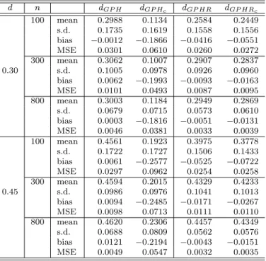
The finite series were simulated from zero-mean ARFIMA models (Eq. 1.2) with {t}t∈Z,t= 1, ..., n, i.i.d. N(0,1). The models, parameters, sample sizes and em- pirical results are displayed in the following tables. The empirical mean, standard deviation (s.d.), bias and mean squared error (MSE) were obtained as a mean of 10.000 replications. The contaminated data were generated from Model 2.3 with m = 1, p = 0.05 for magnitude $ = 10 and bandwidth values for dGP H and dGP HR were computed forα= 0.7 and truncation pointM=n^β,β = 0.7. In the tables dGP Hc and dGP HRc mean the estimates of dwhen the series has outliers.

The simulations were carried out using theOxmatrix programming language (see http://www.doornik.com). The empirical study was divided into the following model properties: stationary and non-stationary processes.

Stationary model

Table 1 displays results for d = 0.3,0.45 and α = β = 0.7. From the table, it can be seen that when the series does not contain outliers, both estimators present similar behavior in the estimation ofd, which is not a surprising result. However, the introduction of outliers in the series dramatically changes the performance of

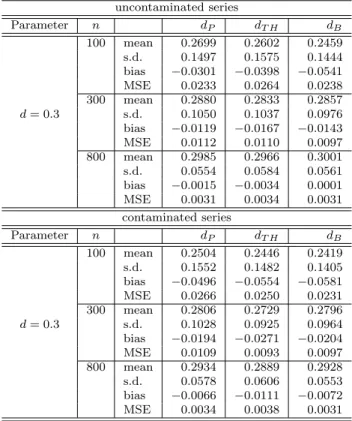
the classical estimator (GPH), in particular, it significantly underestimates the true parameter. On the other hand, in this scenario, the robust method (GPHR) seems to be not sensitive to outliers. Other cases were also simulated such as ARFIMA models with AR and MA parts and different values of p and $. All cases indicated similar conclusions to the one given in Table 1. These are available upon request. Table 2 gives the estimates of d when different lag-windows are used to compute the robust periodogram estimator. The lag-windows are Parzen (P), Tukey-Hamming(TH) and Bartlett (B) and the fractional estimators were computed with the same bandwidths as in the previous case. The choice of the lag-window does not appear to be too important in the estimation ofd since the estimates obtained from different lag-windows are, in general, numerically very close to each other. In other words, the estimates are not too sensitive to the choice of the lag-window. These lag-windows yield similarly accurate estimates compared to the one given in (3.7).

d n dGP H dGP Hc dGP HR dGP HRc

100 mean 0.2988 0.1134 0.2584 0.2449 s.d. 0.1735 0.1619 0.1558 0.1556 bias −0.0012 −0.1866 −0.0416 −0.0551 MSE 0.0301 0.0610 0.0260 0.0272 300 mean 0.3062 0.1007 0.2907 0.2837

0.30 s.d. 0.1005 0.0978 0.0926 0.0960

bias 0.0062 −0.1993 −0.0093 −0.0163 MSE 0.0101 0.0493 0.0087 0.0095 800 mean 0.3003 0.1184 0.2949 0.2869 s.d. 0.0679 0.0715 0.0573 0.0610 bias 0.0003 −0.1816 −0.0051 −0.0131 MSE 0.0046 0.0381 0.0033 0.0039 100 mean 0.4561 0.1923 0.3975 0.3778 s.d. 0.1722 0.1727 0.1506 0.1433 bias 0.0061 −0.2577 −0.0525 −0.0722 MSE 0.0297 0.0962 0.0254 0.0258 300 mean 0.4594 0.2015 0.4329 0.4233

0.45 s.d. 0.0986 0.0976 0.1041 0.1013

bias 0.0094 −0.2485 −0.0171 −0.0267 MSE 0.0098 0.0713 0.0111 0.0110 800 mean 0.4620 0.2306 0.4457 0.4349 s.d. 0.0688 0.0809 0.0562 0.0576 bias 0.0121 −0.2194 −0.0043 −0.0151 MSE 0.0049 0.0547 0.0032 0.0035

Table 1: Simulation results; ARFIMA(0, d,0)model withα=β= 0.7and$= 0,10.

Non-stationary model

As is well-known, the GPH estimator has been widely used even for ARFIMA models with d in (0.5,1.0] (see, for example, Franco & Reisen 2007 [9], Hurvich

& Ray 1995 [15],Olbermann, Lopes & Reisen 2006 [22], Phillips 2007 [24] among

uncontaminated series

Parameter n d_P d_{T H} d_B

100 mean 0.2699 0.2602 0.2459 s.d. 0.1497 0.1575 0.1444 bias −0.0301 −0.0398 −0.0541 MSE 0.0233 0.0264 0.0238 300 mean 0.2880 0.2833 0.2857

d= 0.3 s.d. 0.1050 0.1037 0.0976

bias −0.0119 −0.0167 −0.0143 MSE 0.0112 0.0110 0.0097 800 mean 0.2985 0.2966 0.3001 s.d. 0.0554 0.0584 0.0561 bias −0.0015 −0.0034 0.0001 MSE 0.0031 0.0034 0.0031 contaminated series

Parameter n d_P d_{T H} d_B

100 mean 0.2504 0.2446 0.2419 s.d. 0.1552 0.1482 0.1405 bias −0.0496 −0.0554 −0.0581 MSE 0.0266 0.0250 0.0231 300 mean 0.2806 0.2729 0.2796

d= 0.3 s.d. 0.1028 0.0925 0.0964

bias −0.0194 −0.0271 −0.0204 MSE 0.0109 0.0093 0.0097 800 mean 0.2934 0.2889 0.2928 s.d. 0.0578 0.0606 0.0553 bias −0.0066 −0.0111 −0.0072 MSE 0.0034 0.0038 0.0031

Table 2: Empirical results of d’s estimators in ARFIMA(0, d,0) model using different lag-windows.

others).

Based on the theory discussed in the previous sections, the robust method can not be applied in a non-stationary time series. However, it may be interesting to verify if GPHR estimator is invariant to the first difference, i.e. estimative of the memory parameter based on the original data is equal to one plus the estimatedd based on the differenced data.

Now, let Model 1.2 be defined with parameterd^∗=d+κ, whered∈(−0.5,0.5), κ >0,κ∈Z. Then, Model 1.2, with zero-mean, becomes

Xt= (1−B)^−d∗ηt, t∈Z. (4.4) Process given in (4.4) is non-stationary whend^∗≥0.5; however, it is still persistent.

Ford^∗∈[0.5,1.0)it is level-reverting in the sense that there is no long-run impact of an innovation on the value of the process. The level-reversion property no longer holds whend^∗≥1. Note that whend^∗= 1the process is a random walk.

From Model 4.4 with κ= 1andp=q= 0, Wt= (1−B)Xt, t∈Z,

is an ARF IM A(0, d,0) process. Let dˆ^∗ be the estimator of d^∗ and let dˆbe the fractional estimator obtained from the differenced data. The main goal is to verify the equality dˆ^∗ = ˆd+ 1 for uncontaminated and contaminated series. Based on the same simulation procedure previously described, series from Model 4.4 were generated and some cases are displayed in Table 3 (other cases are available upon request). Similar conclusions to the previous study are observed. Both estimators present equivalent performance when they are applied in the first difference of uncontaminated series. This suggests that both can be used in practical situations when dealing with non-stationary data. However, since the first difference does not eliminate the effect of an outlier, the estimates clearly indicate that caution has to be exercised when there is suspicion of outliers in the data. The GPH estimator presents poor performance in terms of bias (high positive bias) and M SE. In contrast to the GPH estimator, the GPHR method seems to be invariant to the first difference of non-stationary time series with outliers. This empirical study suggests that, in practical situations when dealing with non-stationary data with outliers, one solution is to apply the first difference in the series and then to estimate dwith the robust estimator discussed in this paper.

Parameter n dGP H dGP Hc dGP HR dGP HRc

300 mean −0.2141 −0.5066 −0.1906 −0.2211 dX= 0.8, dW =−0.2 bias 0.0141 0.3066 −0.0094 0.0211 s.d 0.1076 0.1469 0.1127 0.1421 MSE 0.0118 0.1155 0.0128 0.0206 800 mean −0.1906 −0.4283 −0.2062 −0.2250 bias −0.0094 0.2283 0.0062 0.0251 s.d 0.0630 0.0883 0.0851 0.1081 MSE 0.0041 0.0599 0.0073 0.0123 100 mean −0.0048 −0.4166 −0.0449 −0.0871 bias 0.0048 0.4166 0.0449 0.0871 s.d 0.1763 0.2215 0.1620 0.1811 MSE 0.0311 0.2226 0.0283 0.0404 300 mean −0.0122 −0.3230 −0.0273 −0.0426 dX= 1.0, dW = 0.0 bias 0.0122 0.3230 0.0273 0.0426 s.d 0.1076 0.1296 0.1094 0.1277 MSE 0.0117 0.1211 0.0127 0.0181 800 mean 0.0059 −0.2181 −0.0107 −0.0222 bias −0.0059 0.2181 0.0107 0.0222 s.d 0.0648 0.0823 0.0629 0.0909 MSE 0.0042 0.0544 0.0041 0.0088

Table 3: Empirical results: ARFIMA(0, d,0) model with differ- enced data andω= 0,10.

5. Application

IGP-DI is the general price index with domestic availability and is calculated by Fundação Getúlio Vargas, Brazil. The series comprises monthly observations from

August 1994 to April 2011 (total of 201 observations). The series and its ACF are displayed in Figure 1. The observations of the months February 1999 (4.44%), October 2002 (4.21%) and November 2002 (5.84%) are possibly outliers. Looking at the plots in Figure 1, these suggest that the series is stationary and possess long-memory behavior. From the data and using the methodologies previously discussed, the parameter d is estimated and the results are displayed in Table 4. For this application, the estimates of dwere computed from the original data (OD) and from the modified data (MD), where the observations of February 1999, October 2002 and November 2002 were replaced by the sample mean of the series.

This analysis is a simple exercise to verify the robustness of the estimators in a real application and, also, to investigate whether the data contains outliers. The d⁰ estimates of OD and MD series are given, respectively, on the left and right sides of Table 4. These estimates were calculated using different bandwidths in (4.2)(m⁰ = n^α) and β was fixed as in the simulation study. In both series, for a fixed α, the robust methods present similar results. The estimates maintain the same empirical property across the bandwidth values. In contrast to the robust methods, the classical GPH estimator gives estimates that dramatically change from OD to MD data, showing that the observations replaced by the mean are possible atypical data.

time

0 50 100 200

−10123456

0 50 100 150

0.00.40.8

lag

ACF

Figure 1: IGP-DI series and its sample autocorrelation function:

period from Aug/94 to Apr/11.

6. Concluding remarks and future direction

This paper investigates the effect of outliers in the estimation of the fractional pa- rameterdin the ARFIMA(p, d, q) model and, also, discusses the asymptotical and empirical properties of the robust autocovariance and spectral estimators, previ- ously given in Fajardo et al. 2009 [7] and Lévy-Leduc et al. 2011 [19], for the case of time series with short and long-memory properties. These studies support the use

Original time series Modified time series Estimator α= 0.5 α= 0.6 α= 0.7 α= 0.8 α= 0.5 α= 0.6 α= 0.7 α= 0.8 d_{GP H} 0.0757 0.1205 0.3431 0.3759 0.3110 0.3116 0.3713 0.3875

(0.3417) (0.1869) (0.1389) (0.0888) (0.1586) (0.1077) (0.0909) (0.0683) dGP HRP 0.1802 0.2335 0.2269 0.2397 0.1630 0.2077 0.2078 0.2230

(0.0857) (0.0745) (0.0469) (0.0331) (0.0782) (0.0603) (0.0385) (0.0251) dGP HR_{T H} 0.1718 0.1919 0.2125 0.2379 0.1545 0.1782 0.1968 0.2231

(0.0742) (0.0508) (0.0303) (0.0210) (0.0673) (0.0436) (0.0259) (0.0170) dGP HRB 0.1522 0.1788 0.2047 0.2327 0.1379 0.1667 0.1896 0.2181

(0.0641) (0.0433) (0.0262) (0.0183) (0.0586) (0.0378) (0.0227) (0.0151) dGP HR 0.1662 0.2628 0.2454 0.2285 0.1500 0.2211 0.2215 0.2228

(0.0862) (0.0995) (0.0671) (0.0436) (0.0794) (0.0717) (0.0511) (0.0328)

Table 4: Estimates of d: IGP-DI data, period from Aug/94 to Apr/11.

of the robust estimators to estimate the long-memory parameter when Gaussian long-memory time series are contaminated with additive outliers. Non-stationary time series with outliers are also studied and the investigation reveals that the robust method can be used as an alternative estimation procedure in time series with fractional differences. As previously stated, the asymptotical properties of the robust estimator under the study still remain to be investigated. The robust ACF method discussed here has also been used in other contexts such as in the estimation of periodic process (Sarnaglia, Reisen & Lévy-Leduc 2010 [30]) and in seasonal ARFIMA processes (this is one of the current research of the authors).

Acknowledgements. The authors gratefully acknowledge partial financial sup- ports from CNPq-Brazil and FAPES.

References

[1] J. Beran, On a class of M-estimators for gaussian long-memory models,Biometrika, 81:755–766, 1994.

[2] Wai-Sum Chan, A note on time series model specification in the presence outliers, Journal of Applied Statistics, 19:117–124, 1992.

[3] Wai-Sum Chan, Outliers and financial time series modelling: a cautionary note, Mathematics and Computers in Simulation, 39:425–430, 1995.

[4] I. Chang, G. C. Tiao and C. Chen, Estimation of time series parameters in presence of outliers, Technometrics, 30:1936–204, 1988.

[5] C. Chen and Lon-Mu Liu, Joint estimation of model parameters and outlier effects in time series, Journal of the American Statistical Association, 88:284–297, 1993.

[6] P. Doukhan, G. Oppenheim and M. Taqqu,Theory and Applications of Long-Range Dependence, Birkhäuser, 2003.

[7] F. Fajardo, V. A. Reisen and F. Cribari-Neto, Robust estimation in long-memory processes under additive outliers, Journal of Statistical Planning and Inference, 139:2511–2525, 2009.

[8] A. J. Fox, Outliers in time series,Journal of the Royal Statistical Society, 34(B):350–

363, 1972.

[9] G. C. Franco and V. A. Reisen, Bootstrap approaches and confidence intervals for stationary and non-stationary long-range dependence processes, Physica. A., 375:546–562, 2007.

[10] J. Geweke and S. Porter-Hudak, The estimation and application of long memory time series model, Journal of Time Series Analysis, 4:221–238, 1983.

[11] J. R. Hosking, Fractional differencing, Biometrika, 68:165–176, 1981.

[12] P. J. Huber, Robust Statistics, John Wiley & Sons, third edition, 2004.

[13] C. M. Hurvich and K. I. Beltrão, Asymptotics for low-frequency ordinates of the pe- riodogram of a long-memory time series,Journal of Time Series Analysis, 14(5):455–

472, 1993.

[14] C. M. Hurvich, R. Deo and J. Brodsky, The mean square error of geweke and porter- hudak’s estimator of the memory parameter of a long-memory time series, Journal of Time Series Analysis, 19(1):19–46, 1998.

[15] C. M. Hurvich and B. K. Ray, Estimation of the memory parameter for nonstationary or noninvertible fractionally integrated processes, Journal of Time Series Analysis, 16(1):17–42, 1995.

[16] H. R. Künsch, Discrimination between monotonic trends and long-range dependence, Journal of Applied Probability, 23:1025–1030, 1986.

[17] J. Ledolter, The effect of additive outliers on the forecast from arma models, Inter- national Journal of Forecasting, 5:231–240, 1989.

[18] C. Lévy-Leduc, H. Boistard, E. Moulines, M. Taqqu and V. A. Reisen, Large sam- ple behaviour of some well-known robust estimators under long-range dependence, Statistics (Berlin), 45:59–71, 2011.

[19] C. Lévy-Leduc, H. Boistard, E. Moulines, M. Taqqu and V. A. Reisen, Robust estimation of the scale and the autocovariance function of gaussian short and long- range dependent processes, Journal of Time Series Analysis, 32:135–156, 2011.

[20] Y. Ma and M. Genton, Highly robust estimation of the autocovariance function, Journal of Time Series Analysis, 21:663–684, 2000.

[21] R. Maronna, R. D. Martin and V. Yohai, Robust statistics, John Wiley & Sons, 2006.

[22] B. P. Olbermann, S. R. Lopes and V. A. Reisen, Invariance in the first difference in arfima models, Computational Statistics, 21:445–461, 2006.

[23] W. Palma, Long-Memory Time Series: Theory and Methods, Wiley-Interscience, 2007.

[24] P. Phillips, Unit root log periodogram regression,Journal of Econometrics, 138:104–

124, 2007.

[25] M. B. Priestley, Spectral Analysis and Time Series, Academic Press, 1981.

[26] V. A. Reisen, Estimation of the fractional difference parameter in the ARIMA(p, d, q) model using the smoothed periodogram, Journal of Time Series Analysis, 15:335–

350, 1994.

[27] P. M. Robinson, Gaussian semiparametric estimation of long range dependence,The Annals of Statistics, 23:1630–1661, 1995.

[28] P. M. Robinson, Log-periodogram regression of time series with long range depen- dence, The Annals of Statistics, 23:1048–1072, 1995.

[29] P. J. Rousseeuw and C. Croux, Alternatives to the median absolute deviation,Jour- nal of the American Statistical Association, 88:1273–1283, 1993.

[30] A. J. Q. Sarnaglia, V. A. Reisen and C. Lévy-Leduc, Robust estimation of periodic autoregressive processes in the presence of additives outliers,Journal of Multivariate Analysis, 2:2168–2183, 2010.