Simplest mechanical model of stable hopping with inelastic ground-foot impact
Ambrus Zelei∗, Tam´as Insperger∗∗
∗MTA-BME Research Group on Dynamics of Machines and Vehicles
∗∗Department of Applied Mechanics, Budapest University of Technology and Economics and MTA-BME Lendlet Human Balancing
Research Group
Abstract:The dynamic analysis of legged locomotion is challenging because of many reasons, such as the possibly high degrees of freedom of the model, the alternating topology in certain phases of walking or running, the presence of under-actuation and over-actuation, the geometric nonlinearities and ground-foot impact induced non-smoothness. Control issues makes models even more complex, although having models which includes the control strategy of the brain is very helpful in biomechanics. Such models helps to understand how the brain keeps the body in balance, how the energy level is maintained and how the motion patterns are generated.
Before developing a fully extended, very complex model of walking or running, we focus on the dynamic analysis of a piecewise smooth model of hopping, which possesses some fundamental characteristics of locomotion systems: 1) different topology in ground and flight-phase; 2) energy absorption due to partially/fully inelastic ground-foot collision; 3) active control strategy for maintaining a certain energy level; 4) different control strategies in ground and flight-phases.
We prove that our two degrees of freedom model provides stable periodic motion, i.e. vertical hopping in wide range of parameters. We present the application of stability analysis methods that can be adapted for more complex models of legged locomotion.
Keywords:Periodic motion, nonlinear analysis, active control, impact, discontinuities.
1. INTRODUCTION
There are a lot of practically important, open questions about legged locomotion, such as human running. For instance, Souza (2016) directly states: ”At this time, there is limited evidence that any foot strike pattern is more or less likely to cause a runner to sustain an injury”. As another example, Jungers (2010) says ”More studies ... are required to provide data instead of opinion, and testable models and scientific explanation instead of anecdotes.”.
We conclude that reliable mathematical models of legged locomotion are welcomed.
The model based dynamic analysis of legged locomotion is very complex. It involves non-smoothness at foot impacts (Piiroinen and Dankowicz (2005), K¨ovecses and Kov´acs (2011); Zelei et al. (2013)), complex control algorithms (Beer (2009)), delayed control related to human reflex (Stepan (2009)), nonlinearities related to geometrical con- figurations (Seyfarth et al. (2001)) and to saturation of actuators (muscles for human), high degrees-of-freedom (DoF) models, varying topology and alternating over- and under-actuated motions related to the different phases of walking or running.
The implementation and analysis of all these components in a mathematical model is an outstanding challenge.
Because of these difficulties, models currently adopted in biomechanics of legged locomotion are incomplete: most of the existing models are only able to describe experimental results, but important aspects such as balance and control
are generally overlooked, however balancing process can be understood by including a controller that mimics the brain’s operation, see, e.g., Insperger et al. (2013).
Some models which takes into consideration the stability and control are excessively simplified to be applied for humans, like the SLIP model in Holmes et al. (2006).
The model in Rummel and Seyfarth (2008), which has a geometry very similar to the human leg, neglects the mass of leg segments, consequently the important issues of ground-foot collision and impact induced energy ab- sorption are missed. However a considerable amount of energy-demand of locomotion is in relation with ground- foot impact, furthermore foot impact is the main source of injuries when walking and running.
Our long term objective is to develop an integrated math- ematical model for two-legged running locomotion, which includes control, accurate modelling of geometry, and ground-foot impact induced energy absorption. This work considers the analysis of the simplest model for which the same mathematical apparatus is needed as for the more complex models to be developed later.
2. SIMPLEST MODEL OF VERTICAL HOPPING 2.1 Impact induced energy absorption and active control In case of running and hopping robotic or biomechanical systems, some segments of the limbs get in contact with the ground regularly; therefore the motion of these body
12th IFAC Symposium on Robot Control, Budapest, Hungary, August 27-30, 2018.
Paper No. 30.
segments are constrained during the duration of the con- tact. This leads to the absorption of a certain portion of the kinetic energy (Piiroinen and Dankowicz (2005), K¨ovecses and Kov´acs (2011), Zelei et al. (2013)). During the stance- phase, kinetic energy accumulates in the rest of the body as the muscles provide mechanical power, and finally the ground-limb contact terminates.
The model depicted in Fig. 1 is developed for providing the behaviour described above. The particles move with downwards vertical velocity before the end of the flight- phase. The flight-phase ends when particle m2 collides with the ground. Since the collision is fully inelastic in our model, the total amount of the kinetic energy of m2 is absorbed. During the ground-phase the active spring-damper system accelerates m1 in upward vertical direction and increases the total kinetic energy of the system concentrated in m1. In proper case, the hopping height is not lower than the height of the previous hop.
The tuning of the ratio of masses m1 and m2 is crucial.
We introduce m1 =µm and m2 = (1−µ)m with which we express that the portionµof the total mass is included in the upper particle, while the remaining portion (1−µ) is included in the lower particle loosing its total kinetic energy at every touchdown.
The active spring-damper system provides different perfor- mance during the flight- and the ground-phase. Stiffnessk is invariant, but damperdhas a certain positive valuedF in flight-phase in order to suppress undesired oscillations;
while it has a properly chosen negative valuedGin ground- phase in order to regenerate mechanical energy. This op- eration imitates the behaviour of muscles. Since negative damper does not exist in general, the above detailed op- eration can be achieved by using an active actuator in practice.
Fig. 1. Hopping model consists of two vertically moving particles and an active spring-damper placed in grav- itational field above smooth, rigid, horizontal ground.
2.2 Flight- and ground-phase transition discontinuities The system is described by the state variable vector x= [q, q]˙ T, where the vector of general coordinates is q = [z1(t), z2(t)]T. In general q∈ Rn and x ∈R2n. The system dynamics is given by
˙
x(t) =fF(x(t)) and (1)
˙
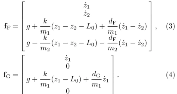
x(t) =fG(x(t)), (2) wherefFandfGare smooth vector fields corresponding to the flight- and the ground-phase respectively. The smooth vector fields are:
fF=
˙ z1
˙ z2
g+ k
m1(z1−z2−L0) + dF
m1( ˙z1−z˙2) g− k
m2(z1−z2−L0)− dF
m2( ˙z1−z˙2)
, (3)
fG=
˙ z1
0 g+ k
m1(z1−L0) + dG
m1z˙1
0
. (4)
We apply parameter µ = m1/m and furthermore we introduce α = p
k/m, DF = dF/(2αm) and DG = dG/(2αm) in order to reduce the number of parameters:
fF=
˙ z1
˙ z2
g+α2
µ(z1−z2−L0) +2DFα
µ ( ˙z1−z˙2) g− α2
1−µ(z1−z2−L0)−2DFα
1−µ( ˙z1−z˙2)
,(5)
fG=
˙ z1
0 g+α2
µ (z1−L0) +2DGα µ z˙1
0
. (6)
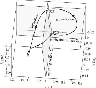
The solution of (1) and (2) goes through smooth vector fields fF and fG which are separated from each other by switching surfaces as it is shown in Fig. 2. Switching surfaces ΣG2F and ΣG2Fare given by the scalar indicator functions hF2G(x) and hG2F(x). Flight to ground (F2G) transition occurs, when surface ΣF2Gdefined by
hF2G(x) =z2 (7)
is crossed from positive to negative direction. Ground to flight (G2F) transition occurs, when set ΣG2Fdefined by
hG2F(x) =λ (8)
is crossed from negative to positive direction. λ is the ground contact force acting on particlem2. Negative and positive sign of λ refers to pushing and pulling force respectively. Here the contact force is a simple expression ofz1and ˙z1, sincez2= 0 and ˙z2= 0 in ground-phase:
λ=−gm2−k(L0−z1+z2) +dG( ˙z1−z˙2) =
=−gm(1−µ)−k(L0−z1) +dGz˙1. (9) In higher DoF systems the contact force can be calculated using the equation
q¨ λ
=
H(q) γTq(q) γq(q) 0
−1
−Q(q)
−γq(q) ˙q
(10) adopted from the book by de Jal´on and Bayo (1994). Here
γq(q) =∂γ(q)
∂q (11)
is the gradient of the geometric constraint vectorγ(q) that represents the ground-foot contact by γ(q) = 0. H(q) is the mass matrix of the unconstrained system andQ(q) is the general force vector of active forces.
2.3 Degrees of discontinuities
Classification of systems according to the degree of discon- tinuity is adopted from the PhD thesis by Leine (2000).
In case of G2F transition, the solution goes through the switching surface without discontinuity, however the vec- tor field changes abruptly and therefore the solution is non-smooth continuous, such as in Filippov-type systems.
On the contrary, F2G transition involves an impact, which cause the discontinuity of the solution: velocity ˙z2becomes zero abruptly when the solution reaches ΣF2G. The jump functiongF2G(x) maps the state into the specified location in the state space (see Dankowicz and Piiroinen (2002)):
gF2G(x) = [z1, z2, z˙1,0]T. (12) In general the velocities are modified by the projectionPa:
gF2G(x) = q
Paq˙
, (13)
where Pa projects into the admissible direction of the constraintsγ in (11) as:
Pa=I−H−1γTq(γqH−1γTq)−1γq, (14) see de Jal´on and Bayo (1994) and K¨ovecses et al. (2003).
Systems with such kind of discontinuities are referred as hybrid systems in Piiroinen and Dankowicz (2005).
3. DYNAMIC ANALYSIS METHOD 3.1 Periodic solution
We focus on hopping motion only, when particle m2 has a larger than zero elevation in the flight-phase; therefore solutions, whenm2is continuously on the ground andm1
has harmonic oscillations are out of our scope.
The beginning of the flight-phase is chosen as the begin- ning of each period, since the state variables z2 = 0 and
˙
z2= 0 are known here att= 0. In other words, we initiate the motion from switching surface ΣG2F. The variable initial values are collected in vector u0= [z1(0),z˙1(0)]T. The smooth solution φF(u0, t) = [φF,1, φF,2,φ˙F,1,φ˙F,2]T of (1) propagates in vector field fF from t = 0 to t = tF2G, when the solution reaches switching surface ΣF2G
indicated by hF2G(φF(u0, t)) = 0. Then jump function gF2G is applied and the state at the beginning of the ground-phase is obtained:
x+F2G(u0) =gF2G(x−F2G(u0)). (15) In alternative interpretation, x+F2G(u0) is the state right after the jump that follows the crossing of ΣG2F. Using similar notation
x−F2G(u0) =φF(u0, tF2G) (16) is the state just before reaching the same switching surface.
After F2G impacting transition, the smooth solution φG(x+F2G(u0), t) = [φG,1,0, φ˙G,1,0]T of (2) continues in vector field fG from t = tF2G to t = tG2F. Note that
solutionφGgoes exactly on ΣF2G, sincez2= 0 and ˙z2= 0 are valid according to (6).
When the solution reaches switching surface ΣG2F, the ground-phase and therefore the full period ends. There is no jump function in the G2F transition, therefore the state right before and after the transition are both
xG2F=φG(x+F2G(u0), tG2F). (17) In state vector xG2F variables z1 and ˙z1 are non-zero only, thus we introduce ue= [φG,1,φ˙G,1]T, which is the intersection point with ΣF2G at the end of each period.
We apply shooting method. The periodic path is found by employing a Newton-Raphson method on the problem F=0, where
F(u0) =ue(u0)−u0. (18) In other words, we find fix pointu∗0 of mappingue(u0).
In case of hopping or running locomotion systems with inelastic ground contact, the dimension of u0 is always lower than the dimensions of the state x, because some state variables (both coordinates and velocities) are known when a limb is contact with the ground.
3.2 Stability analysis integrated in the shooting method One can obtain information about the stability of the peri- odic solution based on the approximation of the Jacobian M(u0) of the solution at the end of the period:
M(u0) = ∂ue(u0)
∂u0
. (19)
This method is quite straightforward to use, since Jacobian J(u0) = ∂F(u0)/∂u0 is necessary to calculate in the Newton-Raphson method, from whichM(u0) is
M(u0) =J(u0) +I, (20) whereIis the identity.
The periodic orbit is stable, if a perturbed initial condition u0is mapped ,,closer” to the periodic path. Thus∀ |µi|<1 is the criterion of asymptotic stability, where µi are the eigenvalues ofM.
3.3 Stability analysis using monodromy matrix
Due to the discontinuities, the accuracy ofM for judging stability of the periodic path is questionable in case of more complex systems. Instead, the computation of the Jacobian of the solution is suggested by Leine (2000) and Piiroinen and Dankowicz (2005). The coupled ODEs (21) and (22) of size 2n + (2n)2 is solved along continuous phases:
˙
x(t) =f(x(t)) ; x(tinit) =x0, (21) Φ(t) =˙ fx(x(t))Φ(t) ; Φ(tinit) =I, (22) whereIis 2n×2nidentity matrix andfx is the gradient of the smooth vector field f. Eq. (22) is referred as first variational equation in the literature.
Equations (21) and (22) are applied with substitutions f = fF, f = fG and tinit = 0, tinit =tF2G in flight- and ground-phase respectively. State flow Jacobians (funda- mental solution matrix in Leine (2000)) ΦF and ΦG are obtained in the flight- and ground-phase respectively.
The Jacobian of the composite solution φ(u0, t) = [φ1, φ,2,φ˙1,φ˙2]T along the whole period needs the Jaco- bian Sof the discontinuity mapping, which is referred as saltation (or jump) matrix in Leine (2000) and in Piiroinen and Dankowicz (2005). Finally, the monodromy matrix, or in other words the composite flow Jacobian at the end of the period is obtained as
Φ(t˜ G2F) =SG2FΦG(tG2F)SF2GΦF(tF2G). (23) Φ(t˜ G2F) can be reliably applied for judging asymptotic stability of periodic orbits, by using criterion ∀ |νi| < 1, whereνi are the eigenvalues of ˜Φ(Floquet-multipliers).
Note that ˜Φ(t) can be used as a Jacobian of the solution φ(x0, t)−φ(xref0 , t)≈Φ(t)˜ x0−xref0
, (24) where φ(x0, t) is the discontinuous solution and ˜Φ(t) is the state flow Jacobian having discontinuities too.
3.4 Computation of saltation matrices
First let us take a look on the G2F transition, where there is no discontinuity mapping of the solution. Here the saltation is given as it is published in the PhD dissertation by Leine (2000):
SG2F=I+(fF−fG)hG2F,x
hG2F,xfG
, (25)
where fF = fF(xG2F), fG = fG(xG2F) and hG2F,x =
∂hG2F/∂x is the gradient of the indicator function eval- uated atxG2F.
In the F2G transition, the discontinuity mapping gF2G
is taken into account and the saltation matrix is calcu- lated according to Dankowicz and Piiroinen (2002) and Piiroinen and Dankowicz (2005):
SF2G=gF2G,x− +
fG+−g−F2G,xfF−) h−F2G,x
h−F2G,xfF− , (26) where fG+ = fG(x+F2G), fF− = fF(x−F2G), h−F2G,x =
∂hF2G/∂x and gF2G,x− = ∂gF2G/∂x are the gradients of the indicator and jump functions respectively evaluated atx−F2G.
4. RESULTS 4.1 Illustration of periodic solutions
The parameters for the numeric example areg= 9.81 [m/s], m= 75 [kg], µ= 0.8 [1],k= 15000 [N/m],dF= 150 [Ns/m], dG=−80 [Ns/m] and L0 = 1 [m] which is the distance of the particles with unstretched spring. The derived parameters are α = 14.14 [1/s], DF = 0.0707 [1], DG =
−0.0377 [1], m1= 60 [kg] andm2= 15 [kg].
Fig. 2 shows a typical periodic solution in the z1, z2 and ˙z1 subspace. The coordinates and the corresponding velocities (sections of the phase-space) are plotted in Fig. 3. Fig. 4 shows the time history of the mechanical energy. The constrained motion space and admissible motion space kinetic energy (CMSKE and AMSKE) can clearly be seen here. CMSKE is absorbed in each F2G transition (see CMSKE in K¨ovecses and Kov´acs (2011)).
Fig. 2. Switching surfaces and a periodic solution. Squares indicate the phase transitions. The circle indicate the intersection with ΣG2F switching surface of the flight-phase solution, which does not have effect on the propagation of the solution. The ground-phase solution goes on ΣF2G. Note: state variable ˙z2 has a jump after reaching ΣF2G, which cannot be seen explicitly here.
Fig. 3. Phase portraits for particle m1 andm2. Here, the jump of state variable ˙z2can be seen. The trajectory of particlem2 in the ground-phase is represented by point G2F.
Fig. 5 shows the elements of M and the time history of some elements of Jacobian ˜Φ(t). ˜Φ(t) were calculated in two alternative ways: the variational equation (22) was
Fig. 4. Time history of kinetic and potential energy.
The absorbed amount of kinetic energy (CMSKE) and the remaining part are indicated by Tc and Ta respectively. The total mechanical energy Etotal
converges to the nominal levelE0 in each jump.
used and besides the estimation was calculated by simply calculating the difference of the perturbed and the periodic solution (see (24)).Mand the solution Jacobian ˜Φat the end of the period and their eigenvalues are
M=
0.0175 0.0024 3.28 0.453
, (27)
Φ(t˜ G2F) =
−0.729 −0.134 −0.248 −0.0634
0 0 0 0
11.41 4.19 3.18 0.803
−11.45 −2.27 −3.84 −0.980
, (28)
µ= [ 0.4714, 0 ], (29)
ν= [ 1, 0.4714, 0, 0 ]. (30) The system is stable with the current parameter set, since the largest relevant eigenvalue isµ1=ν2= 0.4714<1.
4.2 Overview of effect of parameters
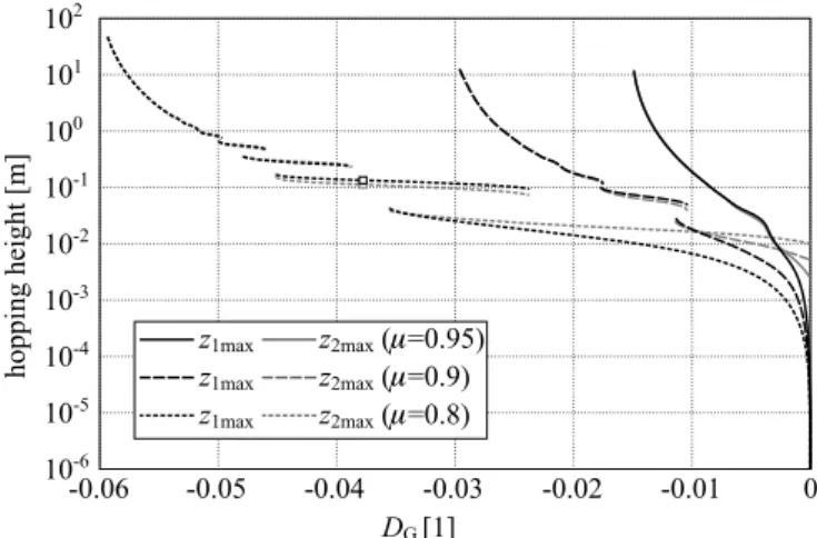
In order to gain an overview of the effect of physical and control parameters, the portion µ of the masses and the negative damping value DG are varied. Parameter µ was set to discrete values 0.8, 0.9 and 0.95. DG was continuously decreased from zero until the system lost stability.
Stable periodic motion was found for all investigated pa- rameter set using simple continuation. Unstable solutions are not presented. Note that more than one stable periodic solution exist for certain parameter sets.
Fig. 6 shows the apex height of the hopping motion.
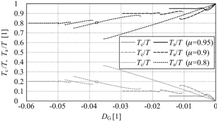
The ratio of CMSKE and AMSKE (absorbed and pre- served amount of kinetic energy) to the total kinetic energy T are plotted in Fig. 7. We can conclude that it is possible
Fig. 5. Time history of elements of Jacobian ˜Φ(t) and elements of M. Dashed black line: ˜Φ(t) calculated by (22), continuous grey line: numerical estimation of ˜Φ(t) by (24). Black crosses: elements of M.
to find optimal parameter set when the ratio of CMSKE is the smallest. This may be a cost function in running and walking systems.
The relevant eigenvalue is plotted in Fig. 8. The results show that the stability highly depends on both physical (µ) and control (DG) parameters. The largest eigenvalue can also be used as a cost function in order to reach robustness.
In some applications, the combination of apex height, robustness and impact intensity may be applied as a cost function.
The above presented results can be reached in case of more complex models of legged locomotion.
Fig. 6. Apex height of the trajectory with different param- eters.
Fig. 7. Ratio of constrained and admissible motion space kinetic energy with different parameters.
Fig. 8. Relevant eigenvalue with different parameters.
5. CONCLUSIONS
We introduced a minimally complex model of hopping that takes into account the inelastic ground-foot impact induced energy absorption and the operation of an active controller maintaining uniform energy level. We demon- strated that stable periodic operation can be achieved in wide range of physical and control parameters. We also showed that it is possible to tune the parameters in order to achieve optimal motion in the sense of lowest foot impact intensity, apex height or robustness.
We adopted a stability analysis method from the literature of piecewise smooth dynamical systems to our model and we concerned the issues of its application for more complex hopping and running models with higher DoF. In future work, these higher DoF and therefore more realistic models of hopping and running will be developed and analysed.
ACKNOWLEDGEMENTS
The research reported in this paper was supported by the Higher Education Excellence Program of the Ministry of Human Capacities in the frame of Biotechnology research area of Budapest University of Technology and Economics (BME FIKP-BIO).
REFERENCES
Beer, R.D. (2009). Beyond control: the dynamics of brain-body-environment interaction in motor systems.
Progress in motor control: a multidisciplinary perspec- tive, ed: Dagmar Sternad (electronic resource), Ad- vances in Experimental Medicine and Biology, 629.
Dankowicz, H.J. and Piiroinen, P.T. (2002). Exploiting discontinuities for stabilization of recurrent motions.
Dynamical Systems, 17(4), 317–342.
de Jal´on, J. and Bayo, E. (1994).Kinematic and dynamic simulation of multibody systems: the real-time challenge.
Springer-Verlag.
Holmes, P., Full, R.J., Koditschek, D.E., and Gucken- heimer, J. (2006). The dynamics of legged locomotion:
Models, analyses, and challenges. SIAM Rev., 48(2), 207–304.
Insperger, T., Milton, J., and Stepan, G. (2013). Acceler- ation feedback improves balancing against reflex delay.
Journal of the Royal Society Interface, 10(79), Article No. 20120763.
Jungers, W.L. (2010). Barefoot running strikes back.
Nature, Biomechanics, 463(7280), 433–434.
K¨ovecses, J. and Kov´acs, L.L. (2011). Foot impact in different modes of running: mechanisms and energy transfer.Procedia IUTAM, Symposium on Human Body Dynamics, 2, 101–108.
K¨ovecses, J., Piedoboeuf, J.C., and Lange, C. (2003). Dy- namic modeling and simulation of constrained robotic systems. IEEE/ASME Transactions on Mechatronics, 2(2), 165–177.
Leine, R.I. (2000). Bifurcations in discontinuous mechan- ical systems of Fillipov type. Ph.D. thesis, Technische Universiteit Eindhoven. ISBN 90-386-2911-7.
Piiroinen, P.T. and Dankowicz, H.J. (2005). Low-cost control of repetitive gait in passive bipedal walkers.
International Journal of Bifurcation and Chaos, 15(6), 1959–1973.
Rummel, J. and Seyfarth, A. (2008). Stable running with segmented legs. The International Journal of Robotics Research, 27(8), 919–934.
Seyfarth, A., G¨unther, M., and Blickhan, R. (2001). Stable operation of an elastic three-segment leg. Biological Cybernetics, 84(5), 365–382.
Souza, R.B. (2016). An evidence-based videotaped run- ning biomechanics analysis. Physical Medicine and Re- habilitation Clinics of North America, 27(1), 217–236.
Stepan, G. (2009). Delay effects in the human sensory system during balancing. Transactions of the Royal Society A, 367(1981), 1195–1212.
Zelei, A., Bencsik, L., Kov´acs, L.L., and Stepan, G. (2013).
Energy efficient walking and running - impact dynamics based on varying geometric constraints. In12th Confer- ence on Dynamical Systems Theory and Applications, 259–270. Lodz, Poland.