stumpf@aut.bme.hu,halasz.sandor@vet.bme.hu BudapestUniversityofTechnologyandEconomics,Dept.ofElectricPowerEngineeringBudapest,Hungary,e-mail: BudapestUniversityofTechnologyandEconomics,Dept.ofAutomationandAppliedInformatics PéterStumpf ,SándorHalász Op

(1)

Optimization of PWM for Overmodulation Region of Two-level Inverters

Péter Stumpf^∗, Sándor Halász^†

∗Budapest University of Technology and Economics, Dept. of Automation and Applied Informatics

† Budapest University of Technology and Economics, Dept. of Electric Power Engineering Budapest, Hungary, e-mail:stumpf@aut.bme.hu, halasz.sandor@vet.bme.hu

Abstract—Three optimized PWM techniques for the overmodulation region of two-level inverter-fed ac drives are introduced and investigated from harmonic loss minimization point of view.

The optimization is elaborated for the lowest loss-factor, which is proportional to the square of rms value of current harmonics.

The loss-factors are computed for different switching numbers as the function of the motor fundamental voltage. It is shown that, respect to the motor heating and torque ripples, the acceptable drive condition can be guaranteed by relatively low value of inverter switching frequency up to 96-97% of maximal possible motor voltage. Furthermore, it is shown that, the so-called Three vector methods have considerably better performance in the lower part of the overmodulation region than the so-called Two vector method for the same number of switching. The performance of the techniques is compared with other existing PWM techniques. The paper discusses the implementation details of the proposed optimal PWM techniques. The theoretical results are verified by experimental and simulation tests.

Index Terms—Pulse width modulated inverters, Optimization methods, Induction machines, Losses, Overmodulation

I. INTRODUCTION

Pulse Width Modulated (PWM) three phase two-level voltage source inverter (VSI) is one of the most common power converter topologies in ac motor drive applications. In the last decades investigation of PWM techniques has been a hotspot in controlling of VSI as they are directly related to the efficiency of the overall system.

The peak of the maximum output phase voltage of a three phase two-level VSI in the so-called six-step or square-wave mode of operation is limited to U_1max = 4U_DC/π, where 2UDC is the DC-link voltage of the inverter. By operating the widely applied standard PWM techniques, like Space Vector Modulation (SVM) or Discontinuous PWM (DPWM) methods, in the so-called linear region, only 90.7% ofU1max

can be reached. Therefore, to improve the DC-link utilization and to expand the output voltage toU1maxthe VSI should be operated in the overmodulation region.

Assuming that, the VSI is supplied by a diode bridge rectifier operating in continuous conduction mode the DC- link voltage in ideal case can be expressed as 2U_DC = 3 ˆULL/π, where UˆLL is the amplitude of the input line- to-line voltage. Hence, the maximum voltage output phase voltage at the border of linear modulation is U₁ = 0.907· 6√

3/π²( ˆULL/√

3) = 0.955( ˆULL/√

3). So mass-produced standard induction machines rated at the input line voltage and frequency would not reach rated operating point in the linear region. It means that, by taking into consideration the voltage drop in the rectifier as well, more than 5% of the

power is inaccessible from a motor fed by a VSI operated only in the linear region [1]. Consecutively, the rated operational point and the flux weakening area of a mass-produced standard induction machines rated at the input line voltage are in the overmodulation region. Thus, the quality of the drive in this region is of great importance.

Recently increasing attention has been paid to high speed induction and synchronous machine drives to reduce system size and improve power conversion efficiency [2]. It poses challenges not only in the field of electric motor design but also in the field of industrial electronics. The basic features of three-phase PWM controlled VSI fed high speed drive are the necessarily high fundamental (synchronous) frequency f₁ (from a few hundred up to thousands) and the limited carrier (switching) frequency f_c (≤15−25 kHz). So a high speed drive system does not only operate at the rated operational point and the flux weakening area in the overmodulation region but the m_f = f_c/f₁ frequency ratio is also a low number (usually mf <21).

It should be noted that, the problems encountered previously with the high speed drives also appear in high-pole count motors, used widely for hybrid and electric vehicles. As in this case the number of poles is high, the required synchronous frequencyf₁can be higher than 1 kHz, while the output speed is a few thousand rpm. Furthermore, in very high power drive systems, the thermal constraints of semiconductor devices also restrict the switching frequency to a few hundred Hz resulting also a very low frequency ratio even at standard f1

fundamental frequencies.

The aim of this paper is to propose and demonstrate harmonic loss optimized PWM control techniques in overmodulation region for low frequency ratios, which makes them applicable to operate high speed, high pole-count drives or high power drive systems in the overmodulation region of good quality.

II. STATE OF THEART

A. Overmodulation

In the linear region of feed-forward (carrier based) space vector based PWM techniques, like SVM, the reference voltage vector has a uniform magnitude and rotates at a constant angular frequency. In the overmodulation region the angle and the magnitude of the reference voltage vector should be modified by passing it through a preprocessor or premodulator [3], [4], [5], [6]. It results in a non-uniform magnitude or non- uniform angular frequency (or both) of the reference voltage vector.

(2)

In the literature two approaches are followed for overmodulation of space vector based PWM techniques. In the first approach, called 2-zone algorithms, the overmodulation region is divided into two zones [3], [6], [7]. The algorithms, called 1-zone algorithms, following the second approach treat the overmodulation range as a single undivided region from the computational point of view [8], [9].

In the case of standard 2-zone algorithm, introduced in [3], in the first part of the overmodulation region (0.907 ≤ m ≤ 0.9514) only the magnitude of reference voltage is modified. In the second part of the overmodulation region (0.9514 ≤m ≤1) both the magnitude and the angle of the reference voltage vector are modified by the premodulator. A modified 2-zone algorithm is presented in [6], [10]. The modified technique has a considerably better harmonic performance than the standard one in the upper part of the overmodulation region as demonstrated in [6]. As different control variables and calculation procedures are used in the two regions, 2-zone algorithms require significant computational effort [9].

In the case of the 1-zone algorithm, introduced in [8], the reference voltage vector has a constant magnitude, but its angle is varied based on simple equations. The advantage of this technique is its simple implementation, however, the low-order harmonic distortion in line currents is much higher than in case of the standard 2-zone algorithm. An improved 1-zone algorithm is introduced in [9], where the magnitude of the voltage vector is also varied by simple equations. It significantly reduces the computational effort comparing to the standard 2-zone algorithm or the standard 1-zone method introduced in [8]. Furthermore, the algorithm reduces the total harmonic distortion in the line current significantly compared to standard 1-zone method. However, the harmonic distortion is still marginally higher than that in case of the standard 2- zone algorithm.

Paper [11] introduces a predictive overmodulation technique in medium-voltage inverters operating at low switching frequencies. A general SVM procedure for overmodulation is described for n-phase drives, where n is an odd number, in [12]. Overmodulation region of inverters is thoroughly studied in closed loop applications [13], [14]. A novel harmonic estimator, which eliminates the unavoidable low order harmonics causing problems in vector controlled drives is described in [13]. Paper [14] presents an overmodulation scheme for sinusoidal PWM used in Field Oriented Controlled (FOC) traction drives, when the switching frequency is only a few hundred Hertz. Overmodulation region of PWM techniques has key importance not only in motor drives but also in grid connected inverters. An overmodulation strategy has been proposed, tested and verified for a 250 kW grid-connected photovoltaic inverter in [15].

In the current paper, similar to [3], the overmodulation region is divided into two regions. They are called as ”Low voltage region” and ”high voltage region” (to be discussed later). From the implementatio point of view, the presented PWM techniques are 1-zone algorithms, as the same calculation procedure can be used for the whole overmodulation region.

B. Optimal PWM

Instead of applying carrier based techniques, programmed modulation strategies can be used as well to control VSIs. In this case the overall approach to define the switching times is based on the minimization of a suitable objective function which typically represents system losses [1]. Applying optimal PWM techniques for ac drive systems has been investigated since the seventies of the last century [16], [17], [18], [19], [20], [21], [22], [23], [24]. An overview of optimal modulation techniques is given in [20]. A space vector based analysis for determining optimal switching angles with reduced computational effort for drives with very low switching frequency for the whole modulation range is introduced in [22]. In [22]

the weighted Total Harmonic Distortion (THD) of voltage is considered for minimization. Paper [23] introduces two algorithms, a frequency domain and a synchronous reference frame based one, to minimize the low-order harmonic torques in induction motor drives, operated at a low frequency ratio.

Paper [25] presents a synchronous optimal PWM method with practical implementation issues for modular multilevel converters. A comparison between time and frequency domain based optimization of PWM techniques is given in [24].

In the current paper the optimization is elaborated for the lowest loss-factor, which is proportional to the square of rms value of current harmonics. In the literature the optimization is mostly done for very small pulse ratios, like5,7 and9. In the current paper the optimization is done for higher, but still low pulse ratios (like 13,15,21,31,43) as well, to obtain a better harmonic performance and drive condition with good quality.

Nowadays, thanks to the high perfomance digital devices, the implementation of optimal methods is considerably sim- pler allowing their wider spread in practice. The paper [26]

demonstrates the use of a digital card flashmemory to follow a preprogrammed optimal PWM pattern. The current paper also discusses the implementation details of the proposed optimal PWM techniques.

C. Loss-factor

The harmonic losses of the machine in the overmodulation region are generally characterized by the loss-factor [27], which can be calculated as follows

K_Ψ⁰ = (σLs)²

∞

X

ν>1

i²_s,ν = Ψ²_s−1 =

∞

X

ν>1

U_s,ν²

U_s,1² ν² (1) where is,ν and Us,ν are the stator current and voltage harmonics of the order ν, respectively. σL_s is the stator transient inductance, where σ = 1− _L^L²^m

sLr, where L_s, L_r and Lm are the stator, rotor and the mutual inductance, respectively. Ψ_s is the rms value of the stator flux. In (1) all the values are in pu system and it was assumed that the machine operates at its rated stator flux. In opposite case (1) should be multipled by Ψ²_s/Ψ²_rated. The base values of the pu system are the rated phase current and voltage, for the flux the ratio U_s,rated/ω_1rated (where ω_1rated is the rated electric synchronous angular velocity) and for the impedance Urated/Irated. Later on, we will use the relative loss-factor K_Ψ =K_Ψ⁰ /0.00215, whereK_Ψ⁰ = 0.00215 is the loss-factor

(3)

(a) mode 1 (b) mode 2,ω1t2=π/12 Fig. 1. Voltage vector path and phase voltage and flux versus time

of the inverter operating in six-step mode [17]. In practice it is desirable to obtain a KΨ loss-factor value lower than0.1 as usually in this case no underrating or additional cooling of the motor is necessary.

D. Optimum solution

The optimum solution means the determination of loss- factor in case of infinitively high switching frequency of the VSI. In overmodulation region, for the fundamental voltage m=U1/Umax>0.907the optimized increase of the voltage can be performed according to [17], [18]. According to the modulation index m = U₁/U_1max, two operational modes are possible. In the first mode (Fig.1(a)) the motor voltage vector U moves along the circle BD₁ with fundamental angular velocity ω1 until it reaches at the t1 time the point D1 of AC line. Then the voltage vector moves along the line D₁D with the same angular velocity ω₁ and at the momentπ/(6ω1)the vector will be inDpoint. The maximum modulation index of the first operational mode, which takes place when D1 point coincidences with A point, can be expressed as m = −√

3 ln(tan(π/6)) = 0.9514 [17], [18].

It should be noted that the first operational mode is the same as ”Overmodulation Mode I” in [3].

In the second operational mode of the investigated π/6 duration the U=πU_1max/3 constant voltage vector stays in the pointAfor the timet2(Fig.1(b)). Att2the voltage vector turns by angleω1t2 inD1 point and moves along D1D line with the constant angular velocityω₁. From Fig.1(b) it can be seen that the difference between the phase voltage or flux and their fundamental components becomes sensible. Therefore, the voltage harmonics and current harmonic losses of this operational mode reach significant values. The anglesω1t1and ω₁t₂ as the function of the modulation indexm=U₁/U_1max can be seen on Fig.2(a).

The second operational mode is similar to ”Overmodulation Mode II” in [3].

The loss-factor is drawn in Fig.2(b). This loss-factor curve is computed asΨ²−1by numerical integration ofΨflux vector [17]. In the first operational mode the loss-factor is very low.

Therefore, it is impossible to distinguish the phase flux from its fundamental component as it can be seen on Fig.1(a) (the flux is given in voltage scale). The maximal K_Ψ = 0.024 value of this mode belongs tom=U1/U1max= 0.9514.

The first eight harmonic voltage components (with correct sign of vector presentation) are presented in Fig.3. Only harmonics of orderν= 1±6Kare possible (K= 0,1,2,3...).

From Fig.3 it can be seen that, in the first operational mode the voltage harmonics for the sameK have the same amplitude.

Angle [rad]

ω₁t₂ ω₁t₁

0.9 0.92 0.94 0.96 0.98 1 π

0 6

π 12

m=U1/U1max (a)ω1t1andω1t2

Loss-factor [pu]

0.9 0.92 0.94 0.96 0.98 1 0

1 0.8 0.6 0.4 0.2

m=U1/U1max (b)KΨ loss-factor Fig. 2. ω1t1 andω1t2angles andK_Ψloss-factor as the function ofm= U1/U1max

The motor harmonic losses as well as the torque pulsation are mainly determined by harmonic currents of order −5 and 7.

These losses decrease sharply with the decrease of the motor voltage. However, the motor torque pulsation really decreases only in the first operational mode. This is clear from Fig.3 since the torque of order 6 is determined by the sum of the torques from currents of order −5 and 7. These torque components have different sign for different sign of voltage harmonics in the second part of the second operational mode (m >0.97). It results in practically constant6^thorder torque component in this region, while the ampltiude of the voltage harmonics changes.

It should be noted that, the conclusions presented previously, assuming infinitively high switching frequency, are valid for multi-level inverters too. Thus, it is impossible to obtain better results than presented above (Fig.2(b)).

m=U1/U1max

Harmonic voltage [pu]

=-5 =7 =-11 =13

0.9 0.92 0.94 0.96 0.98 1

-0.15 -0.1 -0.05 0 0.05 0.1 0.15 0.2

(a)ν= 5,7,11,13

U1/U1maxfundamental voltage

0.9 0.92 0.94 0.96 0.98 1

-0.06 -0.04 -0.02 0 0.02 0.04 0.06

=-17 =19 =-23 =25

(b)ν= 17,19,23,25 Fig. 3. Harmonic voltages for infinitively high switching frequency (γ=∞)

E. Waveform Quality

In the current paper the optimization is elaborated for the lowest loss-factor, which is proportional to the square of rms value of current harmonics (see (1)).

In most cases the optimization is done to minimize the THD

(4)

in line current [1], whereI_{T HD} is defined as IT HD=

sP∞ ν>1i²_s,ν

i²_s,1 , (2)

where i_s,1 is the fundamental current component. It should be noted, IT HD depends on machine parameters. Therefore, in the literature another quantity, the weighted THD of the voltage VW T HD is also applied as a performance index of PWM strategies as it is independent of the motor parameters [1], [6], [5], [22], [28]

VW T HD is defined as V_{W T HD}=

sP∞

ν>1U_s,ν² /ν² U_s,1² =q

K_Ψ⁰ (3) As it can be seen the VW T HD is the square root of the loss-factor. For the proper comparison with other techniques, not only the loss-factor, but theIT HD andVW T HD will also be presented for all investigated optimized PWM techniques.

III. OPTIMIZATION OFPWMFOROVERMODULATION REGION

The computation problem was investigated also in [1], [16], [17], [18], [22], [28]. For a given number of inverter switching and a desiredV fundamental voltage the Lagrange function

F = Ψ²

Ψ²₁−1 +λ(U₁²−V²) (4) must be minimized, where F depends onθi switching (com- mutation) angles and on λ. The computation uses Newton- Raphson method. The computation starts from a given value ofV and a selected voltage vector sequence as well as initial switching angles. It continues until all the first derivatives of F become close to zero. Due to the symmetry of vector paths computations were performed only for0≤ω1t≤π/6 sector (Fig.1), where only U_I = ⁴₃U_DC and U_II = U_Ie^jπ/3 and zero voltage vectors0 and7 can be used.

The number of switching on 1/6^th of the fundamental period is denoted byγ. For a givenγ the number of applying voltage vectors is(γ+ 1)/2, the number of varying switching angles is(γ−1)/2. The total number of angle parameters with θ1= 0,θ_(γ+3)/2=π/6andλis(γ+ 3)/2 + 1.

It should be noted the number of switching over one fundamental period is 6×γ. For the widely applied SVM the number of switching over one fundamental period is6mf. It means that γ has similar meaning as m_f, so it gives the ratio between the switching frequency and the fundamental frequency.

The computations were performed for different number of switching on 1/6^th of the fundamental period: γ = 5,7,9,11,13,15,21,31,43.

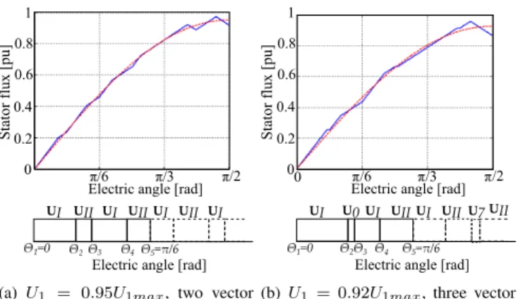
For demonstration the situation for γ = 7 is presented in Fig.4 where the voltage vector sequence in Fig.4(a) is U = [U_I,U_II,U_I,U_II] while in Fig.4(b) it is U = [UI,0,UI,UII]. The stator phase flux, its fundamental component and the applied voltage vector sequence are presented for U1 = 0.95U1max (Fig.4(a)) and for U1 = 0.92U1max

(Fig.4(b)). Later on, the first case, when zero voltage vector is not applied, is called theTwo vector method, and the case,

when zero voltage vector is also applied is called the Three vector method.

Electric angle [rad]

Stator flux [pu] 0.2 0.4 0.6 0.8 1

0

UI

2 3 4

1=0

UII UI UII

5= /6 UI UII UI

/6 /3 /2

(a) U1 = 0.95U1max, two vector method

Stator flux [pu]

0.2 0.4 0.6 0.8 1

0

UI

3

2 4

1=0

U0UI ^UII

5= /6 UI ^UII^U7

/6 /3 /2

0

UII

(b) U1 = 0.92U1max, three vector method, type 1

Fig. 4. Stator phase flux (blue line), its fundamental component (dashed line) and the applied voltage vector sequence,γ= 7

A. Two vector method - ”High voltage region”

This region correspondences to the operation mode 2 in 1(b). The voltage vector path never moves along a fundamental voltage vector path. Therefore, only the two active voltage vectors can be used to obtain a loss-optimal PWM control.

Thus, the zero voltage vectors are not used in this case. This method is introduced in [18]. The same vector sequence is also studied for optimized PWM in [22] for γ = 5,7,9 and 11, where the optimization is done in order to minimizeVW T HD. Later on, the two vector method is abbreviated as 2V.

The calculated optimal switching angles for γ = 13 are presented in Fig.5(a).

Optimal switching angles [rad]

/6

/12

0

Θ1

0.89 0.91 0.93 0.95 0.97 0.99

Θ2 Θ3 Θ4 Θ5

Θ6 Θ7

Θ8

m=U1/U1max (a) Two vector method (2V)

Optimal switching angles [rad]

/6

/12

0 Θ1

0.89 0.91 0.93 0.95 0.97 0.99

Θ2 Θ3

Θ4 Θ5

Θ6 Θ7

Θ8

m=U1/U1max (b) Three vector method, type 1, (3V-T1) Fig. 5. Optimized switching angles,γ= 13

The loss-factors for γ = 5,7,9,11,13,15,21,31 andγ = 43are given in Fig.6. In practice it is desirable to obtain aKΨ

loss-factor value lower than0.1, because the underrating of the motor is usually not necessary in this case. According to Fig.6 the loss-factor is lower than 0.1 only in a narrow region of the motor voltage using two vector method. The performance

(5)

can be improved by increasing γ, however even for γ = 43 it is not possible to obtain loss-factor under0.1 for the whole overmodulation range.

In Fig.7(a) the voltage harmonics of orderν =−5,7,−11 and13are drawn forγ= 13. In this case, whenm≤0.934the first switching angleθ₂= 0, butγ stays13 since atω₁t= 0 there are two switchings (one-one in phases b and c). Figure 7(d) presents the voltage harmonics forγ= 31.

Based on Fig.7(a), Fig.7(d) and Fig.3 it can be concluded that, in them≥0.95region the voltage harmonics have practically the same values forγ= 13(Fig.7(a)),γ= 31(Fig.7(d)) and for infinitively high switching frequency (γ=∞, Fig.3).

Thus, it is worth to optimizing the PWM only in the low voltage region. Furthermore, as the increase of the switching frequency does not change the amplitude of the low order torque harmonics in the m =≥0.95 region, it is impossible to decrease the torque pulsation in sensible rate in this region.

B. Three vector method - ”Low voltage region”

This region correspondences to the operation mode 1 in 1(a). The voltage vector path fromt= 0is moving along U1

vector path, therefore the zero voltage vectors should be used as well. As it will be shown later, by using the zero voltage vectors, the loss-factor values, at least in important part of the voltage region, can be sensibly decreased.

The zero voltage vectors should be applied in the initial part of the voltage vector sequence. In the paper two possible voltage vector sequences are studied: U = [UI,0,UI,UII,UI,UII, ...] and U = [0,UI,UII,UI, ...].

Later on the first one is referred to as type 1 (abbreviated as 3V-T1) and the second one as type 2 (abbreviated as 3V-T2).

As it was mentioned before, due to the symmetry of vector paths, computations were performed only for0≤ω1t≤π/6 sector. It should be noted in the second half of sector 1 (π/6≤ ω₁t≤π/3) the last elements of the voltage vector sequence for3V-T1and3V-T2areU= [...,UI,UII,7,UII]andU= [...,U_I,U_II,7], respectively.

Both3V-T1and3V-T2voltage vector sequences are studied for optimized PWM in [22] forγ= 5,7,9 and11.

The calculated optimal switching angles for γ = 13using 3V-T1are presented in Fig.5(b).

Our results of computations for γ =

5,7,9,11,13,15,21,31 and 43 are presented in Fig.6 and 7, respectively.

It can be seen on Fig.6 that, in the lower part of the overmodulation region the loss-factor for the three vector methods is much smaller than for the two vector method for the same γ. Furthermore, the magnitude of low voltage harmonics (see Fig.7(b)),7(c), 7(e)) became very close to the case ofγ=∞(Fig.3). By comparing the three vector methods 3V-T1and3V-T2, it can be concluded that 3V-T2has a better performance than 3V-T1 in the whole overmodulation range when γ is a small value (see Fig.6(a) when γ = 7). By increasing γ the performance of 3V-T1 becomes better at the beginning of the overmodulation region. By increasing γ this region expands. For example3V-T2is better than 3V-T1 when m > 0.907 if γ = 11. When γ is increased to 21 the performance of3V-T2is better only form >0.945. For larger γvalues the difference between3V-T1and3V-T2in the middle

of the overmodulation region becomes negligible. Therefore, 3V-T1has better performance than3V-T2in the lower part of overmodulation region (m≤0.9514) whenγ >21.

In the upper part of overmodulation region (around m >

0.95) the duration of the zero voltage vector becomes zero consequently the switching number decreases by 4 for 3V- T1 and by2 for 3V-T2. The three vector methods effectively reduce to a two vector method with γ∗ =γ−4 (3V-T1) or γ∗=γ−2 (3V-T2). As it can be seen on 6(a), the loss-factor curve of 3V-T2for γ= 15 andγ = 11for the upper part of the overmodulation region is the same as in the case of 2V when γ= 13andγ= 9, respectively.

Probably for higher value of γ more zero voltage vectors should be used, but according to our calculations for γ≤43 even the use of two zero voltage vectors could not furhter decrease the loss-factor in the overmodulation region.

The voltage vector sequenceU= [0,UI,UII,UI,UII, ...]

is applied for VSI in [23], [29] and in [30] as well, but only for the linear range of modulation. In papers [23], [29]

the technique is called as advanced bus-clamping pulsewidth modulation (ABCPWM) method. In paper [23] the ABCPWM technique is applied and demonstrated for closed loop control of induction machine. Paper [29] proposes a hybrid PWM technique termed as RTRHPWM which employs ABCPWM in conjunction with a conventional switching sequence to reduce pulsating torque and harmonic distortion of line current in induction motor drives. In paper [30] it is demonstrated that this voltage vector sequence can reduce the maximum value of the flux linkage and the core losses in the circulating current filter of parallel connected VSIs.

IV. TORQUE PULSATIONS

The motor torque pulsation is computed by neglecting the motor stator and rotor resistances. In this case the harmonic currents are restricted only by the stator transient reactance, therefore the motor torque pulsation is determined with a good approximation as follows:

∆m= (Ψ_s,1−i_s1,σL_s)×∆i_s, (5) whereΨ_s,1 andi_s,1 is the stator fundamental flux and stator current, respectively. ∆is is the harmonic current vector. In synchronous rotated coordinate system under no-load condition the first term in (5) aligns along imaginary axis. Therefore,

∆m= (Ψs,1−is,1σLs)·∆Re[is] (6) The torque time function is drawn in Fig.8 for γ= 13,31 andγ=∞. It can be seen that, the increase of the switching number can not decrease the6^thtorque component effectively.

At the same time, the use of 3V-T1 leads to an effective decrease of higher order torque components comparing to the 2V method in the lower voltage region (m < 0.95). The frequencies of these two dominant components are3(γ±1)f1, wheref₁ is the fundamental frequency.

Comparing 3V-T1and 3V-T2it can be concluded, the 6^th torque component is considerably lower in the first case.

As it was mentioned previously, three vector methods effectively reduce to a two vector method withγ∗=γ−4(3V-T1) orγ∗=γ−2(3V-T2) in the upper part of the overmodulation

(6)

Loss-factor [pu]

0.9 0.92 0.94 0.96 0.98

0.2 0.8 1

m=U1/U1max 0.4

0.6

0

=5

=7

2V 3V-T1 3V-T2 (a)γ= 5,7

Loss-factor [pu]

0.9 0.92 0.94 0.96 0.98

0.1 0.4

m=U1/U1max 0.2

0.3

0

=9

=11

2V 3V-T1 3V-T2 (b)γ= 9,11

Loss-factor [pu]

2V

0.9 0.92 0.94 0.96 0.98

0.1

m=U1/U1max 3V-T2 0

=13

=15 0.2 0.3

3V-T1 (c)γ= 13,15

Loss-factor [pu]

0.9 0.92 0.94 0.96 0.98

0.2

m=U1/U1max 0.1

0

=21 0.15

0.05 =43 =31

2V 3V-T1 3V-T2 (d)γ= 21,31,43 Fig. 6. Comparison ofKΨloss-factor as the function ofm=U1/U1max

m=U1/U1max

0.89 0.91 0.93 0.95 0.97 -0.1

-0.05 0 0.05 0.1 0.15

0.99 (a) 2V,γ= 13

m=U1/U1max

0.89 0.91 0.93 0.95 0.97 -0.1

-0.05 0 0.05 0.1 0.15

0.99 (b)3V-T1,γ= 13

m=U1/U1max

0.89 0.91 0.93 0.95 0.97

-0.1 -0.05 0 0.05 0.1 0.15

0.9 (c) 3V-T2γ= 13

m=U1/U1max

0.89 0.91 0.93 0.95 0.97 -0.1

-0.05 0 0.05 0.1 0.15

0.99 (d)2V,γ= 31

m=U1/U1max

0.89 0.91 0.93 0.95 0.97 -0.1

-0.05 0 0.05 0.1 0.15

0.99

(e)3V-T1,γ= 31 Fig. 7. Harmonic voltages as the function ofm=U1/U1max

region. Therefore,γ= 9 on Fig.8(b),γ= 11on Fig.8(c) and γ= 27on Fig.8(e), whenm= 0.96and0.98.

V. DIGITALIMPLEMENTATION

The practical aspects of implementing PWM techniques have great importance. The PWM peripheral modules of up- to-date, cheap and powerful microcontrollers (µC) and Digital Signal Processors (DSP) support a wide variety of operation modes and have many features, which makes them proper for motor control applications. Generally these PWM modules consist of an up-down counter, a Period Register (P RD) and three Compare Registers, one for each phase (CM Pi, i=a, b, c).

There are many different approaches to realize commonly used carrier based techniques like SVM. The implementation of the most commonly used SVM in the linear modulation range is straightforward. Generally an Interrupt Service Routin (ISR) is called at the negative or the positive or both peaks of the triangular signal, which calculates the reference signals for each phase. They are latched into theCM Pi (i=a, b, c) of the PWM peripheral to generate the switching signals.

The operation in overmodulation region adds additional complexity, which makes the implementation more difficult.

Some application notes written by the vendors of digital devices suggest some methods for the realization of SVM in the overmodulation region.

In the following, the implementation of the optimized

(7)

Torque [pu]

0.15

0.1 0.05

0 -0.05 -0.1 -0.15

0 0.5

-0.5

Torque [pu]

0.15

0.1 0.05

0 -0.05 -0.1 -0.15

0 0.5

-0.5

Torque [pu]

0.15

0.1 0.05

0 -0.05 -0.1

-0.15-0.5 0 0.5

Torque [pu]

0.15

0.1 0.05

0 -0.05 -0.1 -0.15

0 0.5

-0.5

U1= 0.92 U1max U1= 0.94 U1max U1= 0.96 U1max U1= 0.98 U1max

(a)2V,γ= 13

Torque [pu]

0.15

0.1 0.05

0 -0.05 -0.1 -0.15

0 0.5

-0.5

Torque [pu]

0.15

0.1 0.05

0 -0.05 -0.1 -0.15

0 0.5

-0.5

Torque [pu]

0.15

0.1 0.05

0 -0.05 -0.1 -0.15

0 0.5

-0.5

Torque [pu]

0.15

0.1 0.05

0 -0.05 -0.1 -0.15

0 0.5

-0.5

(b)3V-T1,γ= 13

Torque [pu]

0.15

0.1 0.05

0 -0.05 -0.1

-0.15-0.5 0 0.5

Torque [pu]

0.15

0.1 0.05

0 -0.05 -0.1 -0.15

0 0.5

-0.5

Torque [pu]

0.15

0.1 0.05

0 -0.05 -0.1

-0.15-0.5 0 0.5

Torque [pu]

0.15

0.1 0.05

0 -0.05 -0.1 -0.15

0 0.5

-0.5

(c)3V-T2,γ= 13

Torque [pu]

0.15

0.1 0.05

0 -0.05 -0.1 -0.15

0 0.5

-0.5

Torque [pu]

0.15

0.1 0.05

0 -0.05 -0.1 -0.15

0 0.5

-0.5

Torque [pu]

0.15

0.1 0.05

0 -0.05 -0.1 -0.15

0 0.5

-0.5

Torque [pu]

0.15

0.1 0.05

0 -0.05 -0.1 -0.15

0 0.5

-0.5

(d)2V,γ= 31

Torque [pu]

0.15

0.1 0.05

0 -0.05 -0.1 -0.15

0 0.5

-0.5

Torque [pu]

0.15

0.1 0.05

0 -0.05 -0.1 -0.15

0 0.5

-0.5

Torque [pu]

0.15

0.1 0.05

0 -0.05 -0.1 -0.15

0 0.5

-0.5

Torque [pu]

0.15

0.1 0.05

0 -0.05 -0.1

-0.15-0.5 0 0.5

(e)3V-T1,γ= 31

Torque [pu]

0.15

0.1 0.05 0 -0.05 -0.1

-0.15-0.52 0 0.52

Torque [pu]

0.15

0.1 0.05 0 -0.05 -0.1

-0.15-0.52 0 0.52

Torque [pu]

0.15

0.1 0.05 0 -0.05 -0.1 -0.15

0 0.52

-0.52

Torque [pu]

0.15

0.1 0.05 0 -0.05 -0.1 -0.15

0 0.52

-0.52

(f)γ=∞ Fig. 8. Torque pulsation at no-load

PWM techniques introduced in the paper will be explained.

They are succesfully implemented by the authors on a 16-bit µC (dsPIC33EP512MU810) and on a 32-bit DSP (TMS320F28379D). A few parameters and features of the two devices are listed in Table I.

The angle values calculated offline should be stored in the flash memory of the digital device as a form of a two dimensional array. Each row of the array contains the angles for a given modulation indexm=U1/Umax. The number of rows depends on how many evenly spaced points are defined formbetween the two endpoints of the overmodulation region (0.907 ≤m ≤ 1). We selected the step to be ∆m = 0.001 resulting in ^1−0.907_∆m + 1 = 94 row. By increasing ∆m, the number of rows can be reduced and interpolation can be used to calculate the angles for a certainm value.

Instead of storing the value of the switching angles θ, it is

better to store the duration of the vectors in per unit, which can be calculated as the difference between two consecutive angle values as follows

τ_k= θ_i+1−θ_i

2π , wherej= 1...γ+ 3

2 , k= 1...γ+ 1 2 (7) and θ₁ = 0 andθγ+3

2

=π/6. For a certain f₁ fundamental frequency the duration of the vector in sec can be calculated by multiplying τ_k by the time period T₁ or dividing it by the frequency f1. This way the same array can be used for different f₁ fundamental frequencies.

For the precise operation, the τ_k lengths of the voltage vectors can be stored as a 16/32 bit signed integer number and fixed point arithmetic can be used during calculation. If the processor has Floating Point Unit (FPU) the value of τk

can be stored as 32 bit float number. The required memory can be estimated asM = 32bit·N rOf Rows·N rOf Columns=

(8)

32bit ^0.093_∆m + 1 γ+1 2

. For example for γ= 13 and∆m= 0.001the required memory is approximately2.6kbyte, which is generally much smaller than the available flash memory of the up-to-date digital devices.

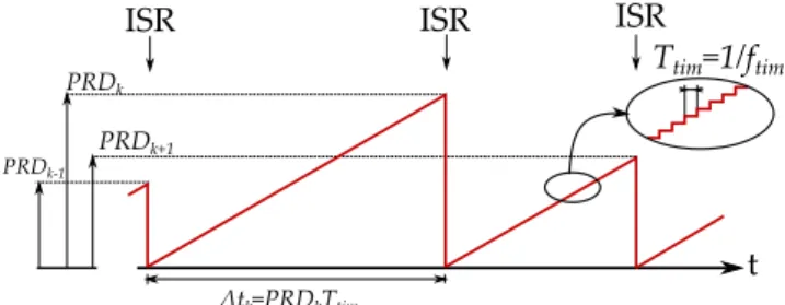
In the overmodulation region, instead of using the up- down counter of the PWM peripheral module, a simple timer (counter) is initialized. Generally the input clock to the timer is derived from the internal clock of the processor, divided by a programmable prescaler. When the timer is enabled, it increments by one on every rising edge of the input clock Ttim and generates an interrupt on a period match, when the counter value equals to the value stored inP RDregister. After period match the timer resets. For the better understanding Fig.

9 illustrates the operation of the timer.

T_tim=1/f_tim ISR ISR

ISR

t

PRDk-1

PRDk

PRDk+1

Δtk=PRDkTtim

Fig. 9. Operation of the timer applied in the overmodulation region

At every period match an ISR function is called (see Fig.

9). As a first step, the duration of the following voltage vector, which is calculated in the previous step, is loaded to theP RD register. Secondly, the switching signals belonging to the voltage vector are generated by manually overriding/forcing the six output pins of the PWM peripheral. Generally the dead time generator is active during the overriding (some vendor called forcing) option as well.

Finally, the next value of the period register is calculated as P RD_k+1=τ_k+1 T₁

Ttim

=τ_k+1f_tim f1

(8) whereftim= 1/Ttim is the frequency of the timer andτk+1

is read from the previously mentioned two dimensional array.

TABLE I

PARAMETERS OF THE APPLIED DIGITAL DEVICES

dsPIC33EP512MU810 TMS320F28379D

CPU frequency 60 MHz 200 MHz

Flash memory 512 kbyte 1 Mbyte

Core size 16 bit 32 bit

FPU no yes

Used Arithmetic fixed point floating point

Price (2017) 9 USD 35 USD

VI. EXPERIMENTAL ANDSIMULATION RESULTS

A. Experimental test using two vector and three vector method To verify the calculation results just described, labora- tory measurements were carried out. Both the two vector and the three vector method were implemented on a 16-bit µC (dsPIC33EP512MU810) and on a 32-bit DSP (TMS320F28379D). The experimental results using the µC are presented in [31]. In the current paper the results using the DSP are introduced.

During the measurement, a commercially available intel- ligent three-phase IGBT module from company Fairchild (FSBB30CH60C) was used for the tests. The VSI is supplied from a single phase diode bridge rectifier, therefore the DC link voltage was2UDC= 320V. The dead time was selected to be 2µs. The torque was measured by an electric torque meter (SILEX TMI-02).

The measurements were carried on an induction machine with rated speed 18 krpm. The rated data and main parameters of the machine are: power:PN = 3kW, rms line-to-line voltage U_{LL,RM S} = 380V, phase rms current I_{N,RM S} = 7.7A, rated frequency f1N = 300 Hz, stator and rotor resistance R_S = 1.125Ω, R_R = 0.85Ω, stator and rotor leakage reactance XLS = 4.71Ω and XLR = 2.63Ω, magnetizing reactanceXm= 84.82Ω(all reactances are at rated frequency) and the number of pole pairs is p= 1.

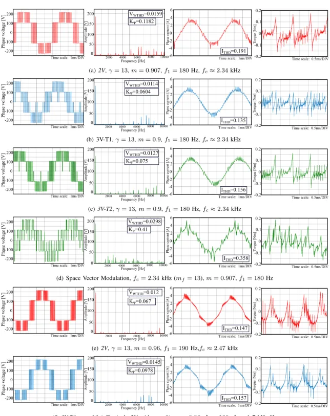
The experimental results at no-load are shown in Fig.10.

For simplicity, the measurements were carried out at lower fundamental frequencies than the rated one. The motor was started using Space Vector Modulation (SVM) algorithm by keeping the ratio U1/f1constant. The overmodulation region was reached at f1= 180Hz, where U1= 0.907U1max. Over f₁ = 180 Hz the proposed optimal PWM strategies were applied.

Figure 10(a), 10(b) and 10(c) present the time function and the harmonic spectra of the motor phase voltage, the time function of the motor phase current and the torque pulsation at f1 = 180Hz and γ= 13 (U1 = 0.907U1max) for the 2V, 3V-T1 and 3V-T2, respectively. The measured WTHD value of the voltage and the THD value of the phase current are also denoted. For a better comparison, the same results were depicted also for SVM on Fig.10(d). The switching frequency for SVM was13·180 = 2.34kHz to obtain the same number of switching over one fundamental period. As it can be seen, 3V-T1and3V-T2have better performance over2Vmethod and SVM algorithm. The influence of the higher voltage harmonics is considerably lower. The peak-to-peak value of the torque pulsation is practically half for 3V-T1 by comparing it with 2V or with3V-T2. The results are in line with the calculated one, presented in the previous section (see Fig.8).

By increasing the fundamental frequency and U1, the performance of 2V becomes better than 3V-T1 or 3V-T2 (see Fig.6(c) and 12(c) later). For example, for γ= 13 it is valid for m≥0.945

By further increasing the fundamental frequency andU1, the duration of the zero voltage vector became zero (for γ = 13 when m≥0.952) consequently3V-T1effectively reduces to a two vector method withγ∗=γ−4(Fig.10(f)). Figure 10(e) and 10(f) show experimental results for m= 0.96(f₁ = 190 Hz). It can be seen that, the harmonic performance of the2V is better than 3V-T1atγ= 13, as the latter one is effectively a two vector method with γ∗= 13−4 = 9.

Fig.11 presents the measured trajectories of the stator current space vectori_sfor3V-T1and3V-T2forγ= 9,13,21and 31atm= 0.92(f1= 183Hz). The THD value of the current signals is also depicted. As it can be seen, the performance of 3V-T1 or 3V-T2 in the lower part of the overmodulation region is acceptable even for low γ values. At m= 0.92 the I_{T HD} value is lower using3V-T2than using3V-T1forγ= 9

(9)

Phase voltage [V]

0 100 200

-200

-100 Phase current [A]

6

Frequency [Hz]

Time scale: 1ms/DIV Time scale: 1ms/DIV

4 2 0 -2 -4 -6

Amplitude [V]

0 50 100 150 200

Torque [Nm]

0.2

Time scale: 0.5ms/DIV 0.1

0

-0.2 -0.1 2000 4000 6000 8000 10000

VWTHD=0.0159

ITHD=0.191 K_Ψ=0.1182

(a) 2V,γ= 13,m= 0.907,f1= 180Hz,fc≈2.34kHz

Phase voltage [V]

0 100 200

-200

6

Frequency [Hz]

4 2 0 -2 -4 -6

Amplitude [V]

0 50 100 150 200

Torque [Nm]

0.2

0

-0.2 -0.1 2000 4000 6000 8000 10000

VWTHD=0.0114

ITHD=0.135 K_Ψ=0.0604

(b) 3V-T1,γ= 13,m= 0.9,f1= 180Hz,fc≈2.34kHz

Phase voltage [V]

0 100 200

-200

6

Frequency [Hz]

4 2 0 -2 -4 -6

Amplitude [V]

0 50 100 150 200

Torque [Nm]

0.2

0

-0.2 -0.1 2000 4000 6000 8000 10000

VWTHD=0.0127

ITHD=0.156 K_Ψ=0.075

(c)3V-T2,γ= 13,m= 0.9,f1= 180Hz,fc≈2.34kHz

Phase voltage [V]

0 100 200

-200

6

Frequency [Hz]

Time scale: 1ms/DIV 2000 Time scale: 1ms/DIV

4 2 0 -2 -4 -6

Amplitude [V]

0 50 100 150 200

4000 6000

Torque [Nm]

0.2

0

-0.2 -0.1 8000 10000

VWTHD=0.0298

ITHD=0.358 K_Ψ=0.41

(d) Space Vector Modulation,fc= 2.34kHz (mf= 13),m= 0.907,f1= 180Hz

Phase voltage [V]

0 100 200

-200

6

Frequency [Hz]

4 2 0 -2 -4 -6

Amplitude [V]

0 50 100 150 200

Torque [Nm]

0.2

0

-0.2 -0.1 2000 4000 6000 8000 10000

VWTHD=0.012

ITHD=0.147 K_Ψ=0.067

(e)2V,γ= 13,m= 0.96,f1= 190Hz,fc≈2.47kHz

Phase voltage [V]

0 100 200

-200

6

Frequency [Hz]

4 2 0 -2 -4 -6

Amplitude [V]

0 50 100 150 200

Torque [Nm]

0.2

0

-0.2 -0.1 2000 4000 6000 8000 10000

VWTHD=0.0145

ITHD=0.157 K=0.0978

(f)3V-T1,γ= 13(effectively2Vwithγ= 9),m= 0.96,f1= 190,fc≈1.7kHz Hz

Fig. 10. Experimental test results at no-load, time function of phase voltage (left), time function of phase current (middle), time function of torque signal and harmonic spectra of phase voltage (right)

is ^[A]

4 2 0 -2 -4 isβ [A]

4 2 0 -2 -4

I_THD=0.185

(a)3V-T1,γ= 9

is ^[A]

4 2 0 -2 -4 isβ [A]

4 0 2 -2 -4

I_THD=0.156

(b)3V-T2,γ= 9

is ^[A]

4 2 0 -2 -4 isβ [A]

4 2 0 -2 -4

I_THD=0.135

(c)3V-T1,γ= 13

is ^[A]

4 2 0 -2 -4 isβ [A]

4 2 0 -2 -4

I_THD=0.122

(d)3V-T2,γ= 13

is ^[A]

4 2 0 -2 -4 isβ [A]

4 0 2 -2 -4

I_THD=0.08

(e) 3V-T1,γ= 21

is ^[A]

4 2 0 -2 -4 isβ [A]

4 2 0 -2 -4

I_THD=0.058

(f)3V-T1,γ= 31 Fig. 11. Experimental test results at no-load, trajectories of the stator current space vector, three vector methods,m= 0.92,f1= 183Hz