TRANSPORT METHODS V

(1)

V

TRANSPORT METHODS

In the previous chapter we discussed the multigroup diffusion methods and their numerical solution. Frequently, however, greater accuracy than that provided by the diffusion equation is demanded by the physical problem. T o this end, one turns to a more accurate relation known as the Boltzmann transport equation. Unfortunately this equation is much more complex and time consuming to solve either analytically or numerically than the diffusion equation.

I n this chapter we consider several special numerical methods for solving the transport equation. Most of the methods considered can be applied to either neutrons or photons. However, some of them will be discussed only for neutrons and others only for gamma rays. T h e development to follow is limited to one dimensional problems. T h i s limitation does not alter the basic approach in any of the methods; however, geometries with several dimensions lead to algebraic complexity.

W e first consider the one group model of the transport equation. W e shall derive the spherical harmonics expansion of the transport equation which leads directly to the PN approximation. W e then consider appro

priate difference equations and alternative procedures for deriving the difference relations. T h e double PN method is then discussed. T h e multigroup transport equations are then derived and an elementary discussion of group cross sections presented. Methods for treating transient problems are then reviewed. Finally we conclude the chapter with a discussion of the moments method.

T h e M o n t e Carlo method is also a way to determine the flow of neutrons and gamma rays. However, this method may be related directly to the transport problem and need not be based directly on the Boltzmann equation. For this reason and because the approach in the M o n t e Carlo method is so very different from that in any of the methods discussed in this chapter, we defer its discussion to the next chapter.

183

(2)

184 V . T R A N S P O R T M E T H O D S

5.1 The ?

N

Approximation

T h e basic equation of neutron conservation is the linear Boltzmann equation.¹ For monoenergetic neutrons this equation is

Ω · V<£(r, Ω ) + at( r ) ^ ( r , Ω ) = 1 dSl' ae(r, Ω ' Ω ) < £ ( Γ , Ω ' ) + S(r, Ω ) ,

J i? (5.1.1)

where <£(r, Ω ) is the number of neutrons crossing a unit surface at r per unit time going in a unit solid angle centered in the direction Ω , at( r ) is the total neutron cross section at r, o~s(r, Ω ' —> Ω ) is the probability per unit length that a neutron at r and going in a direction Ω ' will undergo a collision and emerge going in a unit solid angle centered at Ω , and S ( r , Ω ) is the number of neutrons created per unit volume at r going in a unit solid angle centered at Ω .

Except for a very few special, idealized cases, the Boltzmann equation cannot be solved analytically. T h e term involving the integral is the prime source of difficulty. Accordingly, it behooves us to seek various approximate solutions. Because the integral term involves the angular variable, approximations concerning the angular dependence are sug

gested. W e shall elaborate several of those which have been devised. In particular we shall consider analytic approximations to which numerical procedures may be readily applied.

A particularly useful approximation of the Boltzmann equation is the so-called PN or spherical harmonics approximation. T h e basis of the approximation is the expansion of all functions of the angular variable in terms of the spherical harmonics.² For one dimensional problems, a subset of the spherical harmonics, theLegendre polynomials, suffices. T h e Legendre polynomials are an orthogonal set of functions. T h e flux in the Boltzmann equation may be expanded in terms of these Legendre polynomials. T h e resulting set of equations separates into an infinite set of coupled differential equations. T h e spherical harmonic approximation is introduced by truncating the infinite set of differential equations at some order and treating them by either analytic or numerical methods.

W e shall illustrate the derivation for one dimensional plane geometry.

W e first expand the scattering cross section, directional flux, and the source in Eq. (5.1.1). For an isotropic medium the scattering cross section is a function of only the angle between the vectors Ω ' and Ω , say θ0 . It is convenient to consider the variable cos θ0 == μ0 , rather than

1 For derivations and an elementary discussion, see Appendix A.

2 For properties of the spherical harmonics, see Reference 4, pp. 1325-1328.

(3)

5.1 T H E Pjy A P P R O X I M A T I O N 185

θ0 itself. T h e scattering function can then be expanded in terms of the Legendre polynomials Ρη(μ0). T h u s

<rs(r, Ω ' - Π ) = - i - £ ae.m( r ) P,„(/*o), (5.1.2)

the factor (2m + l)/47r being inserted for later convenience. F r o m the orthogonality of the Legendre polynomials,³ we have

as > w( r ) = 2π f φ0σ8( Γ , Ω ' - > Ω ) Pw( ^0) . (5.1.3)

J - ι

I n slab geometry the flux <£(r, Ω ) will be a function of position χ and, since the medium is assumed isotropic, the angle between the χ axis and Ω , say Θ. It is again convenient to consider the variable cos θ = μ. T h e directional flux is expanded in the form

Η) = Χ ^Γ^Φη(χ) PnM , (5.1.4) η

with

= f άμ4{χ, μ.) Ρη(μ) . (5.1.5)

Likewise, for the source w e have

S(x, μ) = X ^4^- Sⁿ(x) Ρη(μ), (5.1.6) η

with

Sn( * ) = f φ 5 (Λ, μ ) Ρη0 χ ) . (5.1.7)

J - 1

T h e expansions for the directional flux and directional source are func

tions of /x, whereas the scattering function is a function of μ0 . It is evident geometrically that μ and μ0 are related as shown by Fig. 5.1.1.

T h e angles θ, φ refer to the coordinates of Ω , whereas 0', ψ' refer to the vector Ω ' . T h e unit vectors Ω and Ω ' may be written in terms of the unit coordinate vectors as

Ω = cos β i + sin θ cos φ\ + sin θ sin <pk, (5.1.8a)

3 See Appendix D (Eq. D.7) or Reference 3 or 4.

(4)

186 V . T R A N S P O R T M E T H O D S

and

Ω ' = cos 0' i + sin θ' cos φ' j + sin θ' sin φ' k. (5.1.8b) T h e cosine of the angle θ0 is then

cos 0O = fjL0 = cos

θ

cos

θ'

+ sin

θ

sin 0'(cos

φ

cos φ' + sin

φ

sin φ'), (5.1.9a) or

=/(/^x» /A <p') · (5.1.9b)

T o proceed further, the Legendre polynomials Ρη(μ0) with argument μ0

must be expressed as functions of μ and μ . T o this end, the so-called addition theorem for Legendre polynomials is useful (Eq. D.3, Appendix D ) .

F I G . 5.1.1. Geometry of a scattering event

T h e scattering integral in the Boltzmann equation may be reduced to a function of χ, μ only. T h e expansions (5.1.2) and (5.1.4), and the addition theorem may be used in the integrand of the integral in Eq.

(5.1.1). Only the term β = 0 in the sum over β, which arises from the

(5)

5.1 T H E P N A P P R O X I M A T I O N 187

use of the addition theorem, contributes to the integral over φ'. Further, in the integration over μ/, only the combination m = η provides a nonvanishing contribution. By use of the expansions (5.1.4) and (5.1.6) in the remaining three terms of the Boltzmann equation, w e find that

2n + 1

= 2 K « W Ρη(μ) ΦΛΧ) + SH{x) Ρη(μ)] . (5.1.10) η

T o derive the equation for each harmonic, w e multiply (5.1.10) by ΡΝ(μ) and integrate over μ. T h e term in μΡη(μ) is eliminated by use of a recurrence relation for the Legendre polynomials ( E q . D.8, Appendix D ) . After some elementary algebra, w e have

+ σίφη(χ) = σ3.ηφυ(χ) + S„(x), η = 0, 1,.... (5.1.11) Equations (5.1.11) represent an infinite set of coupled differential equations for the harmonics of the flux. Various order approximations are obtained by truncating the series at some fixed Λ⁷. T h e truncation to order Ν consists of assuming all quantities with index Ν + 1 are zero.

T h e first Ν + 1 equations are then used. T h e resulting set of equations are known as the PN equations. T h e Px equations are

-^ΦΙ(Χ) Η"^σίΦο(^χ) =^σβ,οΦο(χ) + S0(x), (5.1.12a) and

1 d

3 άχ^Φο{χ)⁺ σ ί φ ι { χ) = σ β. ^ * ) + · (5.1.12b) T h e P3 equations are

d

άχΦι(χ) + ο·ιφ0(χ) = σ8>0φ0(χ) + S0(x) , (5.1.13a)

2d 1 d

3 dx^φ ^⁺ 3 dx Φο(<Χ>> +σ ί^⁼φ^σ»-^ιΦι(^χ)⁺^SlW > (5.1.13b) 3d 2d

5 d x ⁺ 5 Τχ^φι^⁺^σχί*Μ⁼^σ*ΛΦ*(^χ) + ^S^^x)» t⁵-¹ ·^{1 3 c})

(6)

188 V. T R A N S P O R T M E T H O D S

and

3 d

Tdx^²^⁺^ * )^σ ⁼^σ*.*Φζ(^χ) + SB(x). (5.1.13d) For illustrative purposes we shall use the P3 equations. Higher order

approximations are readily derived, and the results to be obtained sub

sequently are easily generalized.

Because more terms are used in the P3 approximation than in the P1

approximation, the angular distribution can be more accurately repre

sented, and the answers will be more precise. T h e existence of more terms in the P3 approximation than in the Ρλ also implies that the bound

ary conditions can be more accurately approximated. Consistent with the increased accuracy with which the interior of a medium is treated, more accurate boundary conditions are required. Neutron conservation requires that the directional flux be continuous at an interface between two materials. I f the directional fluxes in the adjoining media are denoted φ\χ, μ) and φ^π(χ, μ), then the continuity condition is

φ\χ, μ) = φ"(χ, μ), - 1 < μ < 1 . (5.1.14) In the ΡΝ approximation, it is easily shown that condition (5.1.14)

implies equality of each harmonic of the expansion (see problem 6).

Thus, the boundary condition is

φ'Μ = φ'^χ), allAT. (5.1.15) A t a vacuum-matter interface (or black absorber), the proper boundary

condition is

φ{α9μ)=0, - 1 < / χ< 0 , (5.1.16) where a is the boundary coordinate. Condition (5.1.16) cannot be satis

fied in the PN approximation for finite N. T h e χ directional flux cannot be represented by a finite polynomial expansion. A frequently used boundary condition, which approximates condition (5.1.16), is the Marshak condition

f° άμφ(α)μ)ΡΝ(μ) = 0, TV odd. (5.1.17)

J - 1

A t the opposite boundary for finite slabs, the Marshak condition is

f άμφ(-α,μ)ΡΝ(μ) = 0, Ν odd . (5.1.18)

(7)

5.1 T H E PN A P P R O X I M A T I O N 189 W e shall use the Marshak conditions in our discussion of the PN method.

It should be noted that other approximations have been suggested and applied.⁴ In the next section we consider the double spherical harmonics method which was designed to permit better approximations to dis

continuities in the angular distribution.

T h e application of M a r s h a l s boundary conditions are facilitated by the following relations:⁵

f άμΡη{μ)Ρη{μ)

J η

In like manner, at χ = — ay we obtain

φ0{-α) + 2φ1{-α) +1φ2(-α) = 0 , (5.1.20a) and

φ0(-α) - 5φ2(-α) - Ζφζ(-α) = 0 . (5.1.20b) T h e four conditions at the exterior boundaries, plus the continuity

conditions at interfaces, complete the specification for the P3 approxima

tion. Four boundary conditions suffice, since Eqs. (5.1.13) represent a single fourth order equation. T h i s point may be seen by solving each equation for one unknown (or derivatives of it) in terms of all the others.

T h e result may be used to eliminate this unknown from all other equa

tions, whereupon the process may be repeated again to eliminate another

4 See Reference 1 for a more detailed discussion of boundary conditions.

5 Ε. T . Whittaker and G. N . Watson, ''Modern Analysis," Chapter 15.

Cambridge Univ. Press, London and N e w York, 1940.

T h e Marshak conditions in the P3 approximation are derived in a straightforward manner. F r o m the condition (5.1.17), we find that

(5.1.19a)

(5.1.19b) and

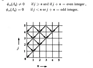
if tn — η

if m — η is even,(w - n ^ O ) if m = 2k, η = 2i + 1

(8)

unknown. T h e boundary conditions (5.1.19) and (5.1.20) play an important role in designing numerical methods for treating the PN

equations. Before turning to the numerical methods, we first illustrate the reduction of the P3 equations to a generalized eigenvalue problem for criticality studies. Once we have obtained the statement of the prob

lem, it is evident that one can define an adjoint function and use the method of successive approximations as detailed in Chapter I V to solve for the flux.

For simplicity we define the coefficients

= σχ — as i = 0, 1,2, 3 .

W e also define the vectors Ψ(Λ:) and S(x) as

Ψ ( * )

'φ0(χ)'

ΦΧ(Χ) φ2(χ)

Μ ^Χ) . and

S(*) =

S0(x) Sl(x) S2(x) S3( * ) J

T h e P3 equations are then written in matrix form Α ψ ( * ) = S ( * ) , with

A =

\_d_

3dx 0

0 d_

dx

σι 2_d_

5 dx 0

2d_

3 dx

0 ~ 2 3d_

1 dx 0

0

3d_

5 dx

(5.1.21)

(5.1.22)

(5.1.23)

(5.1.24)

(5.1.25)

T h e boundary conditions (5.1.19) and (5.1.20) are readily written in matrix form.

For criticality studies there is no external source, only fission. T o an excellent approximation the fission neutron angular distribution is isotropic in laboratory coordinates and further, the fission cross section

(9)

5.1 T H E PN A P P R O X I M A T I O N 191

is independent of the initial neutron direction. T h e source is therefore

S(x, μ) ν J άμ' σϊ(χ)φ(χ, μ) = νσχ(χ) φ0(χ) . (5.1.26)

rFhe expansion coefficients for the source are then S{)(x) - νσχ(χ) φ{)(χ) , and

S,(x) = S2(x) - S,(x) = 0 . T h e P3 equations are then

Α ψ ( * ) = ν Β ψ( χ ) , with

'σ^χ) 0 ··· 0' 0 0

0 0 ο

(5.1.27a)

(5.1.27b)

(5.1.28)

(5.1.29)

Equation (5.1.28) is the general eigenvalue equation we set out to find.

For higher order PN approximations, the formulation is exactly parallel to the above.

W e now consider numerical procedures for solving the equations (5.1.28). T h e continuous space χ, μ, has been replaced by the χ, Ν space where Ν is a discrete variable. In order to derive appropriate difference equations for the harmonics, we again divide the interval —a ^ χ ^ a into discrete points Xj such that xQ = — a , Xj = a. W e again assume the mesh chosen so that all interfaces lie on an interpolation point. T h e discrete mesh appears as shown in Fig. 5.1.2.

T o derive appropriate difference equations, we must consider the boundary conditions applicable to the problem. W e note from Eqs.

(5.1.19) that if any two functions φη(α) are fixed, then the remaining two

N \

3 0 0 1

FI G . 5.1.2. Discrete mesh for the numerical approximation to the P3 equations.

(10)

φη(α) are determined. Likewise for Eqs. (5.1.20). As an example, let us fix φ2(α) and</>3(#); then</>0(a) and φλ(α) are determined. W e now integrate in the direction a to — a to compute φ0( — α) and Φι( — α). But then φ2( — α) αηάφζ( — α) are determined, and hence we should integrate in the direction —a to a to find new values of φ2(α) and φ3(α). Thus a circular path through the mesh is implied, and our difference equations will be derived on this basis. N o t e that the implied direction of integration says nothing whatsoever about the neutron direction.

W e now derive a set of difference equations based upon the above discussion. For the harmonics φ0(χ) and φ^χ), we integrate over the interval Xj to Xj_x . For the equation in φ^χ) we have

Λ^χ j—1 d f^Xj—l C^XJ—l

J ^dx^¹^ ~ J , άχσ0(χ)φ0(χ) = J dxSQ(x). (5.1.30)

W e shall use the double subscript notation

/ „ ( * ; ) = / „ . , . (5-1.31) T h e coefficient σ0(χ) is constant over the interval Xj to χ}_λ and is denoted

G0tj . T h e spacing interval Xj to χ^_λ is denoted

Aj

. T o terms accurate to 0(A)) we have

Φ\,ί-\ —Φυ +^σο . ? y (</>(u-i + Φ0.3) = y ( ^ o . i - i + S o j ) · (5.1.32) T h e equation for φχ(χ) is treated in the same manner; we have

\ fou-i - *⁰. i ) + l (<k,-! - Φυ) + ^ ίΦυ-ι + Φι.,) = 0 · (5.1.33) T h e above difference relations are used for 1 ^ j ^ /.

For the harmonics φ2{χ) and </>3(#), we integrate from Xj to xJ+1 . T h e difference equations are

5 (Φυ+1 — Φΐ,ί)

+ I

(^3,3+1 — Φζ.ι) +^Σ2 , 3 + 1 —γ¹- $2,j+l + Φ2.3) = 0 , (5.1.34) and

η

( ^ 2. i + i — ^2.7) +^σ3, ; + ι W>3,M + ΦΜ) = 0 . (5.1.35) Equations (5.1.34) and (5.1.35) are used for 0 < / — 1.

(11)

T h e direction of integration is shown in Fig. 5.1.3.

Ν

i - ι i j + 2

F I G . 5.1.3. Directions of integration through a mesh for the integration of the Pz equations.

T h e r e are numerous iteration procedures that can be used with the set of difference equations just derived. W e outline one possible procedure below which is analogous to the method of successive displacements.

First we assume an initial distribution for the <f>nj consistent with the boundary conditions. T h e source is computed at each space point.

Starting at/ = /, we solve Eq. (5.1.32) in the form

,1 SQ.J-1 + Sqj + (2/Δ j) (φ°υ

—

< f t L - l ) /l ,c ι

Φο.ί-ι = <PoJ> (DA.00)

where the superscript is the iteration index. Equation (5.1.33) is written as

2 4

= ία rr (Φο·> ~~ ^o.i-i) + Τλ~Ι~~ (Φΐ,ί^— Φ°2,ΐ-ι) — Φι.) · (5.1.37)

Equations (5.1.36) and (5.1.37) are used for 1 ^ j / . T h e analogous equations for the second and third harmonic are

4 6 Φΐ.3+1 =^T~A (Φΐ.) — Φΐ.)+ΐ) +^Τ~Λ (Φζ.ί — Φζ.ί+ΐ) — Φ\.) >

- ^ 3 + 1^σ2. ί+ 1 -^>η)+1^σ2.)+1

(5.1.38) and

Φ*Ί+ι⁼ ία—~ (^2,J^— Φΐ,ΐ+ι) — Φ\.) · (5.1.39) T h e iteration may be repeated for the previously calculated source

5 ° , i.e., multiple inner iterations, or the source may be recomputed from

(12)

the newly found fluxes before continuing. T h e source is rescaled so that (5.1.40) T h e scale factor a² will approach an asymptote after a sufficient number of outer iterations to permit modifications of the assembly properties to achieve criticality. T h e process described above is merely indicative of the types of procedures that are possible.

A n alternative approach to the numerical solution of the PN equations of great merit has been considered by Marchuk (Reference 5, Chapter 13) and Gelbard et al. (Reference 6). W e shall adopt Marchuk's formulation.

It turns out that the PN equations can be reduced to a form identical to that of the multigroup equations. W e shall illustrate this reduction for one case. T h e reduction then enables us to extend the use of any one of the many already existing multigroup diffusion codes to higher order spherical harmonic approximations.

Consider the PN approximation to any order with Ν odd. T h e sources are assumed isotropic. T h e equations are of the form

γχΦι{^χ) +^σοΦο(^χ) = S0(x),

αι + ft ~^Φο(^χ) +^σιΦι(^χ) = 0 ,

+ β N-1 fa<l>N-2(x) +^σΝ-ΐΦΝ-ΐ(^Χ) = 0 , and

β ˝ ^ " - 1 + ˝Φ˝( ) = 0 . (5.1.41) W e define the vectors ψβ( # ) and ψ0( # ) as

~φ0{χ) φ2(χ)

(5.1.42)

and

-Φ˝- (^Χ)Α

~Φι(^χ) φ3(χ)

Ψ«(*) = (5.1.43)

(13)

T h e vector tye(x) contains only even harmonics of the flux, whereas ψ0( # ) contains only odd harmonics. T h e set of equations (5.1.41) may be

written

and

Α , - Ψ Χ Ν ) I- Β^ , Ί * ) = S(A-) ,

Α ^ Ψ Λ * ) + Β2Ψ0( * ) = Ο ,

(5.1.44a)

(5.1.44b)

where the definitions of the matrices are evident upon comparison of Eqs. (5.1.41) and (5.1.44). It is easily seen that the matrices Bx and B2

are diagonal and nonsingular, whereas A1 and A2 are tridiagonal with all diagonal elements zero. N o t e also that A1 and A2 are not functions of x>

whereas Bx and B2 are functions of χ in general. T h e matrix B2 possesses an inverse and hence, from Eq. (5.1.44b),

ψβ( « ) = - Β ^ Α ^ ψ , Ί * ) .

Using the above expression Ί Ο Γ ΨΑ( Λ · ) in (5.1.44a), we have

- ± ( A1B . 7¹A2) ^ ψ „ ( * ) + Β , ψ , Μ = S(x).

(5.1.45)

(5.1.46)

T h e set of equations (5.1.46) are in the same form as the multigroup diffusion equations. In the above case, the harmonic index plays the role of a group index. For the P3 equations, analogous to a two-group diffusion problem, we have

d dx

1 0 2 3 5 5

1

3σλ 3σχ

_3_

7σ3

0

d_

dx φ2(χ)

+

^σ⁰⁰^Φο(φ2(χ) ^χ⁾

S0(x) 0 '

(5.1.47) In detail the equations are

1 d d_

dx Vx [-3—- Τχ (Φο + 2ψ2)] + σ^χ) = S0(x), (5.1.48) and

T h e numerical integration of Eqs. (5.1.48) and (5.1.49) may be done as outlined in Chapter I V .

(14)

A practical advantage of the formulation of the PN equations as multigroup type equations is that a standard multigroup diffusion program is readily used for PN calculations.

5.2 Double P

N

Approximation

T h e PN equations yield quite accurate approximations to the total flux in the interior of a reactor. T h e y should, because the angular dis

tribution deep inside a homogeneous medium is nearly isotropic and because the spherical harmonics method corresponds to an expansion in increasingly higher orders of anisotropy [see Eq. (5.1.4)]. T h e angular distribution deep within a reactor is nearly isotropic essentially because leakage processes, which are anisotropic by nature, do not enter im

portantly into the neutron balance and because nuclear processes, such as fission, tend to be isotropic. Elastic scattering by heavy elements, a predominant process, is isotropic; for the light elements scattering is somewhat anisotropic. However, after a few anisotropic scatterings the angular distribution is nearly isotropic. Consequently, in many cases the angular distribution predicted is therefore good in the interior. However, near strong discontinuities in material properties, such as the region near a strong absorber or vacuum boundaries, the angular distribution is usu

ally much more anisotropic. T h e discontinuities impose step function changes upon the angular flux. T h e approximation of a step function by polynomials requires many harmonics, in particular the P3 approxima

tions would hardly be adequate to represent a discontinuity.

T h e essential idea of the method developed by Y v o n (Reference 7) is to use a separate expansion over each region within which the angular distribution is smoothly and slowly varying, instead of one expansion for all angles. Thus, a discontinuity in the angular distribution can be accurately approximated by using a separate expansion on each side of the discontinuity, the discontinuity being represented by a corresponding discontinuity in the expansion coefficients. In particular, the directional flux is expanded into two series of Legendre polynomials for problems involving an interface between two media. As might be expected, the method of Y v o n is very good for such problems. W e shall discuss the method briefly and reduce the equations to a group diffusion form from which the numerical procedures remaining are evident. Our notation is that of Ziering and Schiff (see Reference 8). W e assume slab geometry and isotropic sources and scattering.

W e begin with the one group transport equation for slabs

d<k(x, μ) + σχφ(χ, μ) = I £ άμ.'σΒ(χ)φ(χ, μ) + ^ . ( 5 . 2 . 1 )

dx

(15)

5.2 D O U B L E Ρ * A P P R O X I M A T I O N 1 9 7

W e expand the directional flux in terms of the half-fange polynomials Ρ+(μ) = Ρη(2μ - 1), 0 < μ < 1 ,

= 0, μ < 0 , (5.2.2a) Ρ » = Ρη(2/* + 1),

= 0, μ > 0 , (5.2.2b) where Ρη(2μ ± 1) is the Legendre polynomial of order n. T h e orthogo

nality relations are

f άμΡ^μ) Pfo) = f χ ΊμΡ,{μ) PJM = ^T+J^δ« » · (⁵·²·³)

T h e half-range polynomials obey the recurrence relation

2(2n + 1) μ Ρ±(μ) = ( » + ! ) Ρ ί+ 1( μ ) ± (2« + 1) Ρ » + n P ± _ » , (5.2.4) a relation that follows from the full range Legendre polynomial recurrence relations. T h e flux expansion is of the form

φ(χ, ,0 = Σ) (2n + 1) [ Ρ » <£+(*) + Ρ ; ( μ ) φ~(χ)], (5.2.5) η

where

φ-(χ) = ί° ^ ( * , /χ) Ρ-(/χ), (5.2.6a)

J -ι

φ+{χ) = \¹άμφ(Χ,μ)Ρϊ(μ). (5.2.6b)

I n view of Eqs. (5.2.2) and (5.2.5), φ* may be regarded as describing the directional flux for μ > 0, and φή(χ), for μ < 0. I f w e insert the expan

sion (5.2.5) into (5.2.1) w e have

£ ( 2 » + 1) μ [ P » ^ # ( * ) + Ρ~(μ) ^Φ~(Χ)]

η

+ at (2n + 1 ) [ Ρ » # ( * ) + Ρ »

•η

W e multiply by Ρ £ ( μ ) and integrate over the interval 0 < μ < 1.

(16)

Again, we multiply Eq. (5.2.7) by Ρ^μ) and integrate with respect to μ over the interval from ± 1 to 0. After some algebra we find

+ 2(2ΛΓ + 1) α,φ^χ) = [ σ . ( * χ ψ ί ( « ) + & ( * ) ) + 2 S0( * ) ] SN 0. (5.2.8)

T h e equations for the double P1 expansion which we denote by Pf are

7ΖΦΛ(^Χ) + ί> ί ( * ) + 2

°ιΦΐ(

^χ

) = ΦΥ&() +*

^{Ψο(*)) +}

2S

⁰

(x),

d x x (5.2.9a) a

3 Τχ^φ+Λχ)⁺ Τχ^φΖ^{χ) + ⁶ ^<* ^⁷^{W =} ° '^{( 5}·²·^{% )} and

- 3

±Kix)

^{+ + fo}^t&"(*) = 0 . (5.2.9d) N o t e that the expansions in φ^{χ) are coupled only through the zeroth

harmonic. For anisotropic scattering the coupling occurs in the higher order terms also.

T h e method of Y v o n makes it possible to satisfy certain types of boundary conditions exactly. A s an example, consider a plane slab in the region — a ^ χ ^ a. A t χ = —α, φ( — α, μ) = 0, 0 ^ μ ^ 1;

at χ = +α, φ(α, μ) = 0, — 1 < μ < 0. T h u s , from Eq. (5.2.6) we learn that the proper boundary conditions are φη{ —^α) = 0 = Φΰ(^α) all η. Since φ^(χ) — 0 for η > Ν + 1, and since we can both require and satisfy φη(—^α) = 0 = Φη(^α)> ^t^e boundary conditions can be ⁿ precisely satisfied. Because the only approximation is the truncation, Y v o n ' s method might be expected to give quite accurate results for this type of problem, as is in fact the case. However, the P^ equations are usually as accurate as the P2N+I equations, particularly with regard to the angular distribution.

T h e set of equations (5.2.9) are readily reduced to a formal multigroup

(17)

5.2 D O U B L E PN A P P R O X I M A T I O N 199 type set of equations. T o this end, we add and subtract the Eqs.

(5.2.9a, c) and (5.}2.9b, d) to obtain the set of equations

d ( t f

(Φί

- Φο) + 2 σ0( ^ + Φο) = 4 S0 , dx

A

dx

3 γ

χ

(Φϊ -ΦΊ) + ί(Φΐ + Φο) + 6a

_dx t

(4t + ΦΊ) = 0 ,

3

^ + ^ + ί

^{{ φ}

° ~

^φ

~

^{ο) +} ⁶ ^σ

^

- * Π = ο , with σ0 = at — σ5 . W e define the vectors

(5.2.10)

and

Ψ.(«) =

Ψ.(*)

(Φΐ-Φι)

(Φί+Φϊ)

(5.2.11a)

(5.2.11b)

T h e set of equations (5.2.10) is then

and

A i ^ W + B ^ x ) = 0 ,

Α2^ Ψ ο Μ + B ^ ) = S ( * ) .

(5.2.12a)

(5.2.12b)

T h e matrix elements are evident. F r o m the first of Eqs. (5.2.12) we have

ψ » = - Β ^ Α ^ ψ , ί * ) , (5.2.13) and hence

- A , ^ [ Β Γ¹^ ^Ve{x)\ + Β2ψ , ( * ) = S ( x ) , (5.2.14)

which is the desired form of the equations. T h e difference equations for the set (5.2.14) are readily formed by methods considered earlier.

(18)

While Y v o n ' s method has not had extensive application, because of its rapid convergence it is useful for treating problems involving sharp changes in material properties for plane boundaries or problems involving the interaction of two plane boundaries.

5.3 Multigroup Transport Methods

T h e derivation of the multigroup transport equations is very similar to the procedure adopted in Chapter I V for the multigroup diffusion equations. T h e basic purpose of this section is to reduce the lethargy dependent Boltzmann equation to a coupled set of transport equations which apply to each lethargy group separately. Once the coupled equa

tions have been found, the remainder of the numerical treatment will be omitted. Instead, various procedures for finding the probabilities for neutron transfer from different groups and angles are considered.

T h e Boltzmann equation with lethargy dependence may be written⁶ Ω · V<£(r, w, Ω ) + at<£(r, w, Ω )

where <£(r, w, Ω ) is the number of neutrons of lethargy u per unit lethargy crossing a unit surface at r per unit time going in a unit solid angle centered in the direction Ω , and as(r; u\ Ω ' ; w, Ω ) is the probability per unit path length that a neutron at r and going in a direction Ω ' with a lethargy u is scattered into a unit solid angle centered at Ω and a unit lethargy interval centered at u. T h e remaining symbols are evident from Section 5.1.

T h e construction of the multigroup equations proceeds as in diffusion theory. W e divide the lethargy range into G groups of arbitrary width and label the initial and final lethargies as 0 = w0 , wth = uG . T h e thermal group is indexed by G -f- 1. L e t Aug = ug — ug_x . W e then integrate Eq. (5.3.1) from ug_x to ug to obtain

Ω - V ^ ( r , Ω ) + oJ(r, Ω ) ^ ( Γ , Ω ) = Q*(r, Ω ) + S' ( r , **)> * = 1, 2 , G .

Ω '

Λ Ω^,[ σ8( Γ; κ ' , Ω ' ; κ , Ω) ψ ( Γ , Μ ' , Ω ' ) ] + S{r, w, Ω ) , (5.3.1)

(5.3.2) W e let

6 The derivation of (5.3.1) is in Appendix A .

(19)

5.3 M U L T I G R O U P T R A N S P O R T M E T H O D S 201 T h e averages are all weighted by the appropriate flux. Thus, for at(r,w) we use

i[ ( r , Ω ) = f⁹ dua^v, u) φ(τ, u, Ω ) / f° άηφ(ν, u, Ω ) , (5.3.4) whereas for Q(r, u, Ω ) we use

Q°(r,Sl) =

f°

^ ρ ( τ , « , Ω ) ^ ( Γ , « , Ω ) / Ρ ^ ( Γ , « , Ω) . (5.3.5)

T h e thermal equation may be added to the set (5.3.2) in the form

Ω · V < ^ + \ r , Ω ) + a f+ ^ r ) < £^{G + 1}( r , Ω ) = 0^{G + 1}( r , Ω ) + S^ r , Ω ). (5.3.6) T h e set (5.3.2) plus the thermal group equation and the boundary conditions furnish a multigroup transport formulation which is rigorous.

T h e remaining steps are approximate, and each step is taken to reduce the complexity of the problem. T h e first problem is obtaining the appropriate group constants. Obviously weighting with the flux and even the directional flux is a time consuming process. M a n y alternative procedures have been suggested including: (1) use of infinite media spectra to eliminate iterative determination of group constants; (2) use of the fission spectrum as the weighting function; (3) use of diffusion theory spectra; (4) constant flux within groups and hence unweighted cross sections. W e do not specify any procedure at the moment, but assume the group constants may be specified at the beginning of the computation.

T h e second problem is the relation of the average flux to the flux at the lethargy interfaces. A full range of possibilities exists as in diffusion theory. W e shall use only one approximation, namely

^ ( r , Ω ) = φ(τ,ησ, Ω ) = <^(r, Ω ) , (5.3.7)

which is accurate only to order Δη. Likewise for the other variables.

T h e group equations are then

Ω · V ^ ( r , Ω ) + o* ( r ) ^ ( r , Ω ) = ρ * (Γ, Ω ) + S' ( r , Ω ) , £ = 1 , 2 , G + 1.

(5.3.8) N o t e that the angular dependence of σ\ has been dropped; σ9χ must be only slightly dependent on Ω as may be seen from Eq. (5.3.4), if the multigroup approximation (5.3.7) is a good one, since the total cross section itself is nearly independent of Ω .

(20)

T h e set of Eqs. (5.3.8) is the multigroup transport equations desired.

T h e nature of the inhomogeneities will be considered in the remainder of this section. W e shall describe a few ways of calculating them in detail.

T o this end, we observe that the set of equations (5.3.8) is equivalent to the assumption

f '

duK(u) = <x«K',

(5.3.9)

ug-l

where OL is a constant which depends upon the weighting function assumed for the lethargy dependent constants, and K(u) is a lethargy dependent variable. For instance,

f° dua

t

(r,

«)<£(r,

u,0) =

a% [ ( r ) ^ ( r , f t ) . (5.3.10)

T h e terms of particular interest are the inhomogeneous terms Q^g(r, Ω ) and S^g(r, Ω ) . W e consider first the scattering source Q°(r> Ω ) .

F r o m Eq. (5.3.9) we have

o^ ( r , Ω ) =

Γ° duQ(r,

« , Ω ) . (5.3.11)

T h e integration over u' may be written as a sum

άη'σ8(τ;η\^;ηιςΐ)φ(τίη\ςΐ')=ν^σΙ\τ;^;η^)φ^(τ^')) (5.3.12) where σ ? ' ( Γ , Ω ' ; u, Ω ) is the probability that a neutron at r going in the

direction Ω ' in the group g' will suffer a scattering in going a unit distance and be scattered into a unit solid angle centered at Ω and a unit lethargy centered at u. T h e integration of (5.3.12) over the interval uQ_x to ug

yields

G+l

OL J <#’ < > ' ( r , Ω ' ; Ω ) < ^ ' ( r , Ω ' ) , (5.3.13) g'=i

and hence

Q

⁹

(r,

Ω )

=

V

<#>

f o f.'(r, Ω ' ; Ω ) ^ ' ( Γ , Ω ' ) , (5.3.14)

where

σ

⁹3

'>°

is the probability of transfer from group

g'

with direction Ω '

(21)

5.3 M U L T I G R O U P T R A N S P O R T M E T H O D S 203

to group

g

with direction Ω . T h e nature of the coefficient

o°

s

'>

^g depends upon the materials within the assembly and the nature of the scattering law. For instance, if no upscattering is permitted, then

< · ' = 0 , if*' >g. (5.3.15) For elastic scattering of heavy elements, then, only terms for g' near g

enter.

W e now consider the source term S^ff(r, Ω ) . W e again have

Γ" duS(r, u> Ω ) = oL*S«(r, Ω ) . (5.3.16)

T h e source will consist of fission sources plus extraneous sources. T h e fission sources are

Sf(r, w, Ω ) = vX(u) j du' j d£l'at(r\ u\ Ω ' ; w, Ω)φ(τ, U\ Ω ' ) . (5.3.17)

T h e integration over u' is replaced by a summation to yield

Sf(r, u, Ω ) = vX(u) d& V

cfi'afir,

^{Ω ' ; u,} Ω ) ^ ' ( Γ, Ω ' ) . (5.3.18)

W e then have

S J ( r , n ) = νχΨ^' ί » ; ^ Ω ' ; Ω ) ^ , Ω ' ) . (5.3.19)

T h e equations (5.3.14) and (5.3.19) imply that the right-hand side of Eq. (5.3.8) is

where S% is the external source and

T°'>°{r; Ω ' ; Ω ) = a* ' [ < '^y + νχ,σ?'.'].

Τ^σ'>^σ(τ; Ω ' ; Ω ) is called the transfer kernel for the multigroup equations.

Physically T°'*^a(r\ Ω ' ; Ω ) is the probability that a neutron appears in group g going in a unit solid angle centered at Ω as a result of a neutron in group g' at r going a unit distance in a unit solid angle centered at Ω ' . T h e function T^Q,*^Q may be constructed after the relevant scattering

(22)

laws and cross section weighting factors have been chosen. A s an exam

ple, consider the case of isotropic scattering and fission in the laboratory coordinates. T h e scattering kernel is then of the form

T»'.'(r; Ω ' ; Ω ) = i - T''>«{r). (5.3.20)

It is frequently useful to expand the transfer kernel in Legendre polynomials. I f the cosine of the angle between Ω ' and Ω is μ0 , then we expand T^a'*° in the form

7 V. ' ( r ; Ω ' ; Ω ) = ± - £ ^ ± _ L jv,,{t) W . (5.3.21) η

T h e zeroth harmonic contains the isotropic components while the re

maining harmonics include the anisotropic moments.

T h e angular and spatial variations are separable under certain con

ditions, e.g., for isotropic media. T h e transfer kernel may then be written

Τ°'<"(ν, Ω ' ; Ω ) = C ° ' > ' ( r ) Ω ) . (5.3.22)

C⁹'>⁰(r) is the probability that a neutron appear in g r o u p s as a result of a neutron in g r o u p s at r going a unit distance. For one group problems, the coefficient is merely C( r ) , the mean number of neutrons per collision. W e shall make frequent use of Eq. (5.3.22) in the remainder of this chapter.

5.4 Discrete Ordinate Methods

In Section 5.1 we considered approximate solutions to the transport equation by use of an expansion in terms of Legendre polynomials. In particular the angle variable was eliminated from the equation in favor of harmonic coefficients. W e now consider an alternative treatment of the angular dependence called the discrete ordinate method. W e will merely outline the procedure for developing discrete ordinate approxima

tions. In the next section we specialize to a particular method, the SN

method. T h e reason for the emphasis on the SN method is due to its wide use in transport calculations.

For simplicity w e consider the one group transport equation in slab geometry with isotropic scattering

(23)

5.4 D I S C R E T E O R D I N A T E M E T H O D S 205

W e have used the transfer kernel of the previous section, and hence the source Se(x, μ) is external.

Rather than expand the flux, we divide the μ interval into a discrete number of intervals instead, hence the name discrete ordinate. L e t the interpolation points be denoted as μη , η = 0, 1, Ν. T h e directional flux is to be evaluated at the points μη and interpolated in between. W e denote directional fluxes φ(χ, μη) = φη(χ). N o t e the subscript η now refers to a given direction, not an index for an expansion.

T h e transfer integral is now approximated by a quadrature formula of the form

f άμ'φ(χ,μ')=Σ™η*>Φη>(χ), (5.4.2)

where the wn, are weighting factors. T h e Boltzmann equation is applied to each group separately in the form

d c( x} ·*. \

n'

(5.4.3) I n order to avoid discontinuities the interpolation points are so chosen that μη Φ 0, all η.

A variety of quadrature formulas have been proposed and used. I n particular, for interfaces where the directional flux may be discontinuous at μ = 0, double expansions in μ space are recommended. T h e most frequently suggested method for such problems is Gauss quadrature.

T h i s method has significant advantages regarding the accuracy of the approximation. T h e use of the Gaussian quadrature was suggested by W i c k (Reference 9 ) .

I n the elementary integration formulas considered in Chapter I I I , it was indicated that Ν point integration formulas approximated the integrand as a polynomial of degree Ν — I. T h e Gaussian integration formula has the property of being accurate to order 2N, i.e., approxi

mating the integrand as a polynomial of degree 2N — 1. T h e remarkable feature of this quadrature is that only Appoints are needed for the integrand.

I n order to derive the Gaussian quadrature, w e consider the following problem. Suppose w e have a polynomial f2N-i(^x) ° f degree 2N — 1.

Is it possible to find another polynomial, of degree Ν — 1, gw-i(^x)y which agrees with f2N-i(^x)^a^t Ν points, say Xj , j = 1, 2, N, and such that

f « f r/ 2 w - i( * ) = f (5.4.4)

J - 1^J - 1

(24)

206 V. T R A N S P O R T M E T H O D S

for properly chosen Xj ? I f the above question can be answered in the affirmative, then the integration of gN-i(x) can be replaced by a summa

tion which gives exactly the value of the integral. In other words, it is then possible to approximate an integral with an iV-point formula which has a truncation error of order 2N.

T h e proof that such an integration formula is possible is simple.

Since f2N-i{^x)^l^s ° f order 2N — 1 .and gN-x(x) coincides with f2N-i(^x)^a^t Ν points xn , we have

Ϊ2Ν-ι(^χ) = Sn-i(^x) + (x- Xi)(x - x2) - (x - xn) Gn-i(x) > (5.4.5)

where GN_ i ( # ) is a polynomial of degree Ν — 1. I f w e integrate Eq.

(5.4.5) from — 1 < χ < 1 and apply (5.4.4), then we must have

f dx(x — Xj)(x — x2)... (x — xN) GN -1 = 0 . (5.4.6)

J - 1

I f the integration formula is to be valid for all /2ΛΤ-Ι(*)> then GA r_1( j c ) is arbitrary. Hence each power of χ in 0Ν_τ(χ) which appears in (5.4.6) must vanish separately. T h a t is,

ί dx(x — xj(x — x2)... (Λ: — xN) xⁿ = 0, η = 0, 1, ..., Ν — I . (5.4.7) J - 1

T h e coefficient of xⁿ in the above integral is a polynomial of degree N, and Eq. (5.4.7) states that this polynomial must be orthogonal to all polynomials of lower degree, over the interval — 1 ^ χ ^ 1. It is well known that the Legendre polynomials satisfy this criterion. Therefore, if the interpolation points are the zeros of the Legendre polynomial of degree Ny then Eq. (5.4.7) and thus Eq. (5.4.4) are true. But then we have

Γ¹ ^

dxf2N-i(x) = 2J^wif2N-i(Xj) > (5.4.8)

which is exact. W e now consider finding the Wj. First consider f2N-i(^x) — constant. T h e n

X w, = 2 . (5.4.9)

3=1

(25)

5.4 D I S C R E T E O R D I N A T E M E T H O D S 207

By continuing in this manner we arrive at a set of Ν simultaneous equations of the form

"1 1 . . 1 " " ^ 1 "

xx #2 •^XN x\ •^X~N ^ο ^•

=

X*

*

x^N

(5.4.10)

where the cn are readily formed by inserting various powers of χ into Eq.

(5.4.8). Since the rows of the square matrix in Eq. (5.4.10) are linearly independent, the inverse matrix always exists, and the Wj may be found by solving Eq. (5.4.10). In fact it is readily shown that the weight factors are always positive (see problem 10). T h e r e are several other formulas that can be used to derive the weight coefficients Wj (see, for instance, Reference 70, pp. 362-367).

T h e example we have used to derive the Gaussian integration formula was a particularly simple one. T h e r e exist many Gaussian formulas for different intervals of integration, and for more complicated integrands.

W e will not have occasion to use the more general formulas (for further details, see References 10 and 11).

T o reiterate, the advantage of the Gaussian quadrature is the high order truncation error. A disadvantage is the location of the interpolation points. T h e intervals are not equally spaced in general, and for this reason the Gaussian type formula is rarely used for deriving difference approximations. Nevertheless for integration over the angular coordinate, the method is frequently used. It can be shown (see Reference 2, pp.

268-271) that for spherically symmetric scattering the discrete ordinate method using Gaussian quadrature is equivalent to the spherical har

monics method.

T h e discrete ordinate equations, Eqs. (5.4.3), are readily reduced to finite difference equations by standard techniques. In the next section a particular example of the formation of the spatial difference equations will be given in conjunction with the SN method. A s a final word on the discrete ordinate method, we remark that anisotropic scattering can be incorporated into the equations, and multigroup problems considered.

T h e discrete ordinate method is widely used for one dimensional problems; its use in multidimensional problems seems to have been limited.

(26)

5.5 The Method

T h e SN method is a special case of the discrete ordinate method and was originated by B. G. Carlson (see Reference 12). T h e characteristic feature of the SN method is the assumption of linear variation of the directional flux between interpolation points in both the angular and spatial variations. W e shall derive the equations in a straightforward manner for spherical geometry in the multigroup model. Consideration is then given to a variant of the SN method, called the discrete SN

method, also proposed by Carlson (Reference 13).

T h e transport equation for a given energy group g in spherical geom

etry is⁷

μ ±φ»(,,

μ)+1(1-

^/χ²) §-^{r, μ) + σ>ψ>{τ, μ) = S'(r), (5.5.1) where μ is the cosine of the angle between the neutron direction and the radius vector where we have assumed all sources are isotropic. A n isotropic source is not an essential feature of the SN method but it greatly simplifies the analysis. T h e extension to include anisotropics is direct but detailed, and we shall not consider such problems here. T h e interval

— 1 ^ μ ^ 1 is divided into Ν segments, usually of equal width, Δη . T h e interpolation points are then defined as μη = — 1 + 2n/N so that μ0= — 1 and μΝ = \. T h e directional flux is assumed to vary linearly between the interpolation points, and hence

f (r, μ) =^μ - φ»(τ, μ») + μ η_λ ), (5.5.2)

for /χη_! ^ μ ^ μη . A representative directional flux distribution is shown in Fig. 5.5.1 for an 54 approximation.

Here

Φη(χ) = Φ&, μη) · (5.5.2a)

T h e linear approximation in Eq. (5.5.2) may be substituted into Eq.

(5.5.1) and the result integrated from μη_χ to μη . T h e integration yields

Κ Tr + Τ⁺^σ'1 ^ ⁽ ^r) + Κ Ί~Τ⁺ =^C»^S'^{J { r )}'

(η = 1,2, ..., ΛΤ) (5.5.3)

7 For derivation see Appendix A.

(27)

5.5 T H E M E T H O D 209 with

an = ^ (2μ„ + μη-ι) . «M "= ^ (Μ,/ + 2^r t..j)

^fi = - j j - (³ — — / ^ i i - l — » and

Cn = 2 .

- 1 -1/2 0 1/2 1 /i

F I G . 5.5.1. SA approximation to the directional flux distribution. The dashed line represents the directional flux; the solid line, the approximation.

T h e set of equations (5.5.3) consists of Ν equations in the Ν + 1 unknowns <f>an(r). T h e Ν + 1st equation is obtained by setting μ = — 1 and writing the transport equation, Eq. (5.5.1), directly. W e have

-±4ψ)+

= S»{r). (5.5.4)

T h e above equation may be included in the set (5.5.3) by choosing the constants

«o = - ¹ >

*o = 0 ,

Φ'-ιΜ = 0 ,

Ό = 1 .

It is evident that the approximations made are accurate to order (Αμ²).

T h e spatial dependence is obtained in the same manner. W e divide the interval 0 ^ r ^ R into / segments of width Aj = rj — r^_x, which are not assumed equal. As usual the division is such that interfaces lie on

(28)

interpolation points. W e order the points such that r0 = 0, tj = R. T h e mesh in r — μ space for any energy group is shown in Fig. 5.5.2.

1 Ν

Μ η

Λ 0

0 0

J r

J R F I G . 5.5.2. Mesh in r — μ space for an .S4 calculation.

In order to perform the spatial integrations, it is important to consider the direction of neutron motion. For the line μ = — 1, i.e., η = 0, the neutrons move from large r to small r. For reduced truncation error, we should perform the spatial integration in the direction of neutron travel (see problem 11).

T o derive the appropriate difference equations for η such that μη ^ 0, we integrate from r$ to r$_x . Conversely, for μη > 0, we integrate from τ3_λ to Yj . L e t Aj be defined as Aj = — r^_x . T o terms of order A* we approximate integrals as

f>

^* ^/ ^{W =}

/ < ^ i ^ U .

( 5 . 5 . 5 ) T h e terms in 1/r are integrated by assuming an average value l/<^>.

T h e simplest choice is < r;) = (r^ + r;-_i)/2 = fj . Another choice is

<r*> = f

3

T h e difference equations for η = 0, 1, Af/2 are found by integrating ( 5 . 5 . 6 )

TRANSPORT METHODS V

V