Global Description of Action-Angle Duality for a Poisson–Lie Deformation of the

c 2019 The Author(s) 1424-0637/19/041217-46 published onlineMarch 6, 2019

https://doi.org/10.1007/s00023-019-00782-7 Annales Henri Poincar´e

Global Description of Action-Angle Duality for a Poisson–Lie Deformation of the

Trigonometric BC n Sutherland System

L. Feh´er and I. Marshall

Abstract. Integrable many-body systems of Ruijsenaars–Schneider–van Diejen type displaying action-angle duality are derived by Hamiltonian reduction of the Heisenberg double of the Poisson–Lie group SU(2n).

New global models of the reduced phase space are described, revealing non-trivial features of the two systems in duality with one another. For example, after establishing that the symplectic vector spaceCⁿ R²ⁿ underlies both global models, it is seen that for both systems the action variables generate the standard torus action onCⁿ, and the fixed point of this action corresponds to the unique equilibrium positions of the per- tinent systems. The systems in duality are found to be non-degenerate in the sense that the functional dimension of the Poisson algebra of their conserved quantities is equal to half the dimension of the phase space.

The dual of the deformed Sutherland system is shown to be a limiting case of a van Diejen system.

Contents

1. Introduction 1218

2. Preparations 1223

2.1. The Master System and Its Reduction 1223

2.2. The Model ˆM ofMred and Its Consequences 1227 3. Constructing the Model M ofMred: General Outline 1230

4. A Useful Characterization of the SpaceN 1235

5. Solution of the Constraints 1239

6. The Global ModelM ofMredand Consequences 1247

6.1. Construction of the ModelM ofMred 1248

6.2. Consequences of the Model ofM and the Duality Map 1251

7. Discussion and Outlook 1253

Acknowledgements 1255

A Some Explicit Formulae 1255

B The Relation ofH (1.11) to van Diejen’s Hamiltonian 1256

References 1259

1. Introduction

Integrable Hamiltonian systems have important applications in diverse fields of physics and are in the focus of intense investigation by a great variety of mathematical methods. We are interested in the family of classical many-body systems introduced in their simplest form by Calogero [2], Sutherland [38] and Ruijsenaars and Schneider [35]. The relevance of these systems to numerous areas of mathematics and physics is apparent from the reviews devoted to them [4,21–23,31,34,39,42]. One of their fascinating features is that several pairs of such systems enjoy a duality relation that converts the particle positions of one system into the action variables of the other system, and vice versa.¹ This intriguing phenomenon was first analyzed in the ground-breaking papers [30,33] by a direct method, while its group theoretic background came to light more recently [14,15,21]. The treatment of the self-dual Calogero system by Kazhdan et al. [16] served as a source of inspiration for these developments.

Since this paper is devoted to the analysis of a particular dual pair, let us next outline in more precise terms the notion of duality that we use.

An integrable Hamiltonian system is given by an Abelian Poisson algebra Hof smooth functions on a 2n-dimensional symplectic manifold (M, ω) such that the functional dimension ofHis n, and all elements of Hgenerate com- plete flows. The systems of our interest possess another distinguished Abelian Poisson algebraP, which has the same properties as Hand the following re- quirements hold:

(a) There exist Darboux coordinates, λ_i, θ_j, on a dense open submanifold M^o ofM such that the restriction ofP toM^o is functionally generated by theλi.

(b) H contains a distinguished function H whose restriction to M^o admits interpretation as a many-body Hamiltonian describing the dynamics of ninteracting ‘point-particles’ with positionsλi moving along one dimen- sional space (a line or a circle).

The function H is often called the ‘main Hamiltonian’ and P is sometimes called the algebra of ‘global position variables’.

Now, suppose that we have two systems

(M, ω,H,P, H) and ( ˆM ,ω,ˆ Hˆ,Pˆ,H),ˆ (1.1)

1Self-duality occurs when the related systems are identical, except for a possible shift of their parameters.

with associated Darboux coordinates, according to conditions (a) and (b), (λ, θ) and (ˆλ,θ). We say that these two systems are in action-angle dualityˆ (also called Ruijsenaars duality) if there exists a global symplectomorphism R: (M, ω)→( ˆM ,ω) such thatˆ

H= ˆP◦ R and Hˆ =P◦ R⁻¹. (1.2) An additional feature, valid in all known examples, is that the Hamiltonian flows of (M, ω,P) and ( ˆM ,ω,ˆ Pˆ) can be written down explicitly, not only on the dense open parts, but globally. Consequently, (M, ω,H) is integrated by means of ( ˆM ,ω,ˆ P), and ( ˆˆ M ,ω,ˆ H) is integrated by means of (M, ω,ˆ P). This means thatRandR⁻¹can be interpreted as global action-angle maps for the Liouville integrable systems (M, ω,H) and ( ˆM ,ω,ˆ Hˆ). One may also say that ˆP represents global position-type variables for the many-body system ( ˆM ,ω,ˆ Hˆ) and global action-type variables for the system (M, ω, H), together with the analogous ‘dual statement’.

For further description of this curious notion and its quantum mechan- ical counterpart, alias the celebrated bispectral property [3], the reader may consult the reviews [31,34]. We note in passing that in some examples theλi

are globally smooth and independent, and thenM^o=M, while in other exam- ples, they lose their smoothness or independence outside a proper submanifold M^o. This should not come as a surprise since from the dual viewpoint theλ_i are action variables, which usually exhibit some singularities. Their canonical conjugatesθ_i may vary on the circle or on the line depending on the example.

It was realized by Gorsky and his collaborators [14,15,21], and explored in detail by others [5–13,24,25], that dual pairs of integrable many-body sys- tems can be derived by Hamiltonian reduction utilizing the following mech- anism. Suppose that we have a higher dimensional ‘master phase space’ M that admits a symmetry groupG, and two distinguished independent Abelian Poisson algebrasH¹ andH² formed byG-invariant, smooth functions on M.

Then we can apply Hamiltonian reduction toM and obtain a reduced phase space Mred equipped with two Abelian Poisson algebras H¹_red andH²_red that descend, respectively, fromH¹andH². We need to construct two distinct mod- elsM and ˆM of Mred yielding (M, ω,H,P) and ( ˆM ,ω,ˆ H,ˆ P) in such a wayˆ that the reduction ofH¹ is represented by Hand ˆP, and the reduction ofH² is represented byP and ˆH. If this is achieved, then we obtain a natural map R: M → Mˆ that corresponds to the identity map on Mred and relates the Abelian Poisson algebras onM to those on ˆM in the way stated in (1.2). (See also Fig. 1, placed at the end of the section.) A crucial, and very intricate, requirement is that the reduction must provide many-body systems: to fulfill this, one can rely only on experience and inspiration. The heart of the matter is the choice of the correct master system and its specific reduction. The ex- amples so far treated by the mechanism just outlined include group theoretic reinterpretations of dual pairs previously constructed by direct methods as well as new dual pairs found by reduction. At the same time, there still exist such known instances of dualities as well (notably, the self-dual hyperbolic RS

system [30] and the dual pair involving the relativistic Toda system [32]) that stubbornly resist treatment in the reduction framework.

The crucial advantage of the above-outlined approach to action-angle dualities is that, once the correct starting point is found, the Hamiltonian re- duction automatically gives rise to complete flows and symplectomorphisms between the models of the reduced phase space. For the realization of this advantage, it is indispensable to provide globally valid descriptions of the re- duced system, which can be a thorny issue. The solution to such global issues is at the heart of our current investigation.

The goal of this paper is to present a thorough analysis of a dual pair of integrable many-body systems recently derived in [8,13] by reduction of the Heisenberg double of the standard Poisson–Lie group SU(2n). It is well-known [36,37] that the Heisenberg doubles are Poisson–Lie analogues (and deforma- tions) of corresponding cotangent bundles. The relevant reduction is a direct Poisson–Lie generalization—making use of Lu’s momentum map, [18]—of the reduction of the cotangent bundleT^∗SU(2n) used for deriving the trigonomet- ric BC_n Sutherland system and its dual in [7]. Correspondingly, the reduction of the Heisenberg double leads to a deformation of this dual pair. We shall not only describe the deformed dual pair, but shall also show how duality allows us to extract non-trivial information about the dynamics. For example, it will allow us to prove that both of the resulting integrable many-body Hamiltoni- ans are non-degenerate since their flows densely fill the corresponding Liouville tori. Furthermore, it will be shown that all the flows of Hposses a common fixed point, as do the flows of ˆH. These results will be established by utilizing the global descriptions of the dual models M and ˆM of the reduced phase space.

Our current line of research was initiated in the paper [19], where the analogous reduction of the Heisenberg double of SU(n, n) was considered. The investigation in [7] was strongly influenced by the work of Pusztai [25], who studied a dual pair arising from reduction of T^∗SU(n, n). The Poisson–Lie counterpart of the SU(n, n) dual pair appears more complicated than what we report on here; its exploration is left for the future.

Before outlining the content of the paper, let us recall from [8,13] the lo- cal description of our many-body systems in duality, which arises by restricting attention to dense open submanifolds of the reduced phase space. These sys- tems have 3 real parameters,μ >0 anduandv, whose range will be specified below. Here, we use hatted letters to describe the model constructed in [8].

The manifold ˆM contains a dense open proper subset ˆM^oparametrized by the Cartesian product

D+×Tⁿ={(ˆλ,exp(iˆθ))}, (1.3) whereTⁿ is ann-torus and

D+={ˆλ∈Rⁿ |min(0, v−u)>ˆλ₁>· · ·>λˆ_n, ˆλ_j−λˆ_j+1> μ, j= 1, . . . , n−1}. (1.4)

The ˆλ_i and the angles ˆθ_i are Darboux coordinates, i.e., on ˆM^owe have ˆ

ω= n j=1

dˆθj∧dˆλj. (1.5)

The main Hamiltonian ˆH can be written on ˆM^o as H(ˆˆ λ,θ) =ˆ U(ˆλ)−

n j=1

cos(ˆθj)U1(ˆλj)^1/2 n (k=j)k=1

1− sinh²μ sinh²(ˆλj−ˆλk)

1/2

(1.6)

with

U(ˆλ) =e^−2u+e^2v 2

n j=1

exp(−2ˆλj), U₁(ˆλ_j) =

1−(1 +e^2(v−u)) exp(−2ˆλ_j) +e^2(v−u)exp(−4ˆλ_j) .

(1.7)

The phase spaceM of the ‘dual model’ possesses a dense open proper subset M^o parametrized by

D+×Tⁿ={(λ,exp(iθ))} (1.8)

with

D+={λ∈Rⁿ |λ₁>· · ·> λ_n >max(|v|,|u|), λ_j−λ_j+1> μ, j= 1, . . . , n−1}. (1.9) It carries the Darboux form

ω= n j=1

dθj∧dλj. (1.10)

In terms of these variables, the main HamiltonianH reads H(λ, θ) =V(λ) +e^v−u

n j=1

cosθj

cosh²λj

1− sinh²v sinh²λj

1/2

1− sinh²u sinh²λj

1/2

× n (k=j)k=1

1− sinh²μ sinh²(λ_j−λ_k)

1/2

1− sinh²μ sinh²(λ_j+λ_k)

1/2

(1.11) with

V(λ) =e^v−u

⎛

⎝sinh(v) sinh(u) sinh²μ

n j=1

1− sinh²μ sinh²λj

−cos(v) cosh(u) sinh²μ

n j=1

1 + sinh²μ cosh²λj

+C0

⎞

⎠ (1.12)

where C₀=ne^u−v+cosh(v−u)

sinh²μ . The constantC₀ is included here for later convenience.

The formulae of the main Hamiltonians ˆH (1.6) andH (1.11) are invari- ant with respect to the independent transformations μ → −μ and (u, v) → (−v,−u). Motivated by this, we assume throughout the paper thatμ >0 and at a later stage we shall also assume that

|u|>|v|. (1.13)

The exclusion of |u| =|v| is required for our reduction treatment, while the choice (1.13) turns out to have technical advantages. The above-specified do- mains D+ and D+ emerge from the reduction, but they can also be viewed as choices made to guarantee the strict positivity of all expressions under the square roots appearing in the Hamiltonians.

A few remarks are now in order. The main Hamiltonians ˆH andH are reminiscent of many-body Hamiltonians introduced by van Diejen [40]. The relation regarding ˆH was made precise in [8] and regardingH it will be de- scribed in this paper. The coordinates ˆλi andλiserve as position variables for Hˆ andH, respectively, and we shall see that they yield globally smooth (and analytic) functions on the underlying phase space. Note that the deformation parameter that brings this dual pair into the one obtained by reduction of T^∗SU(2n) [7] is here set to unity. The cotangent bundle limits of ˆH andH are discussed in [8] and in [13].

Now we outline the content of the paper and highlight our main results.

In Sect.2.1, we first recall the Heisenberg doubleMequipped with the Abelian Poisson algebrasH¹ andH², then set up the pertinent reduction. In Sect.2.2, we review the global model ˆM of the reduced phase space found in [8]. The material in Sect.2 enhances several previous results. For instance, Lemma2.1 and the relation (2.46) ofH^red_j to Chebyshev polynomials appear here for the first time. Section 3 contains the logical outline of the construction of the global modelM, which is our primary task. This is summarized by Fig. 2at the end of Sect. 3. The elaboration of the details required new ideas and a certain amount of labor: it occupies Sects. 4, 5 and 6.1. Our first main re- sult is Theorem5.6in Sect.5. Crucially, this theorem establishes the range of theλ-variables that arises from the reduction. Building on the local results of [13], it also yields the Darboux chart (1.10) on a dense open submanifold of Mredparametrized by (1.9). Our second main result is given by Theorem6.5, which describes the symplectomorphism Ψ between (M, ω), cast as Cⁿ with its canonical symplectic structure, and (Mred, ωred). Combining Theorem 6.5 with previous developments, we explain in Sect. 6.2 that our reduction en- genders a realization of the diagrams of Fig. 1. We consider this to be our principal achievement. We also present consequences for the dynamics of the systems in duality in Sects.6.2and 7. Section7 is devoted to further discus- sion of the results and open problems. Finally, two appendices are included.

The first one is purely technical, while in the second we clarify the connection between the HamiltonianH (1.11) and van Diejen’s five parametric integrable trigonometric Hamiltonians.

M0 M

M Mred Mˆ

Rⁿ Rⁿ

ψ π0 ψˆ

ι0

λ R

Ψˆ Ψ

ˆλ

ι^∗₀(H¹)×ι^∗₀(H²)

H×P H¹_red×H²_red Pˆ ×Hˆ

ψ^∗ Ψ^∗

π^∗0

Ψˆ^∗ ψˆ^∗

R^∗

Figure 1. Illustration of how symplectic reduction is used to generate duality. These diagrams are designed to help keep track of the notations. Using the embeddingι0:M0→ Mof the ‘constraint surface’M0 into the master phase space M, the reduced Abelian algebras are defined byHⁱ_red◦π₀=Hⁱ◦ι₀ fori= 1,2. They turn into the Abelian algebras of the models M and ˆM according toH◦Ψ =H¹_red = ˆP◦Ψ andˆ P◦Ψ = H²_red= ˆH◦Ψˆ

2. Preparations

In this section we set up the reduction of our interest and review the model Mˆ of the reduced phase space. All manifolds in this article are viewed as real.

Hence the expression “analytic” must always be understood to mean “real- analytic”. We shall focus on theC^∞ character of the manifolds and maps of our concern, but shall often also indicate their analytic nature by parenthetical remarks.

2.1. The Master System and Its Reduction

We shall reduce the master phase spaceM := SL(2n,C). Here, SL(2n,C) is viewed as a real Lie group, and we also need its subgroups

K:= SU(2n), B:= SB(2n), (2.1)

where the latter is formed by upper triangular complex matrices with posi- tive entries along the diagonal. Every element g∈ M admits the alternative Iwasawa decompositions

g=kb=bLkR, k, kR∈K, b, bL∈B. (2.2) By using these,Mis equipped with the Alekseev–Malkin [1] symplectic form

ω_M=1

2tr(dbLb⁻¹_L ∧dkk⁻¹) +1

2tr(b⁻¹db∧k⁻¹_R dkR). (2.3) To display the corresponding Poisson bracket, for any F ∈ C^∞(M,R) we introduce the sl(2n,C)-valued left- and right-derivatives∇F and∇F by

d ds

s=0

F(e^sXge^sY) =tr

X∇F(g) +Y∇F(g)

, ∀X, Y ∈sl(2n,C). (2.4)

We prepare the linear operator R= 1

2(π_K−π_B) (2.5)

on sl(2n,C), utilizing the projectors associated with the real vector space de- composition

sl(2n,C) =K+B, (2.6)

where K and B are the Lie algebras of K and B, respectively. The Poisson bracket reads

{F,H}=tr (∇FR(∇H) +∇FR(∇H)), F,H ∈C^∞(M,R). (2.7) The structure described above is known [36,37] as the Heisenberg double of the standard Poisson–Lie group SU(2n).

The Abelian Poisson algebra H² is defined as follows. LetP denote the space of positive definite Hermitian matrices of size 2n and determinant 1.

Consider the ringC^∞(P)^Kof smooth real function onPthat are invariant with respect to the natural action ofK onP given by conjugation of a Hermitian matrix by a unitary one. We set

H²={H ∈ˆ C^∞(M)|H(g) = ˆˆ h(bb^†) with ˆh∈C^∞(P)^K}, (2.8) i.e.,H² is the pull-back ofC^∞(P)^K by the mapM g→bb^† ∈ P. A gener- ating set ˆHj forH²is provided by the functions ˆHj having the form

Hˆj(g) = ˆh_j(bb^†) with ˆh_j(bb^†) := 1 2tr

(bb^†)^j

forj = 1, . . . ,2n−1. (2.9) The Hamiltonian vector field and the corresponding (complete) flow can be written down explicitly for any ˆH ∈H². After our reduction thenHamiltonians descending from the functions ˆH1,Hˆ2, . . . ,Hˆn remain independent, and the many-body Hamiltonian displayed in (1.6) results from ˆH1.

To present the other Abelian Poisson algebra of interest,H¹, we define the matrix

I:= diag(1n,−1n), (2.10) where1n is then×nunit matrix, and introduce the subgroup

K+:={k∈K|k^†Ik=I}. (2.11) LetC^∞(K)^K+×K+denote those functions onKthat are invariant with respect to both left- and right-multiplications by elements ofK₊. Then, referring to the Iwasawa decomposition (2.2), we define

H¹={H ∈C^∞(M)| H(g) =h(k) withh∈C^∞(K)^K+×K+}. (2.12) A generating set is furnished by the functionsHj given by

Hj(g) =h_j(k) withh_j(k) := 1 2tr

(k^†IkI)^j

forj= 1, . . . , n. (2.13) We recall thatC^∞(K) carries a natural Poisson bracket associated with (2.7), for which the mapg→kby (2.2) is a Poisson map. Explicitly,

{f, h}K(k) =tr

Df(k)k(Dh(k))k⁻¹

, ∀k∈K, f, h∈C^∞(K). (2.14)

Here theB-valued left- and right-derivatives,Df andDf, of anyf ∈C^∞(K) are defined analogously to (2.4). It is well-known thatKis a Poisson–Lie group and K₊ < K is a Poisson–Lie subgroup of K with respect to this Poisson structure. The following lemma implies thatH¹is an Abelian Poisson algebra.

Lemma 2.1. The invariant functions C^∞(K)^K+×K+ Poisson commute with respect to{,}K.

Proof. Let us start by noting that everyk∈K may be written in the form k=κ1Δκ2, forκ1, κ2∈K+, and Δ =

Γ iΣ iΣ Γ

, (2.15) where

Γ = diag(cosq1, . . . ,cosqn), Σ = diag(sinq1, . . . ,sinqn) (2.16)

with π

2 ≥q1≥q2≥ · · · ≥qn ≥0. (2.17) Ifh1 andh2are two (K+×K+)-invariant smooth functions onK, then their Poisson bracket is also (K+×K+)-invariant. Therefore it is enough to show that{h1, h2}vanishes at any point of the form Δ given in (2.15).

The (K+×K+)-invariance ofh∈C^∞(K) means that theB-valued left- and right-derivativesDh, Dhhave the form

Dh=

0 A

0 0

, Dh=

0 A˜

0 0

, (2.18)

where we use the obvious 2×2 block-structure defined byI(2.10). On account of the identity

Dh(k) =π_B(k(Dh(k))k^†) =k(Dh(k))k^†−π_K(k(Dh(k))k^†), (2.19) we must also have

Dh(k)−k^†(Dh(k))k∈ K. (2.20) Applying this atk= Δ, we obtain

−iΓAΣ A˜−ΓAΓ

−ΣAΣ iΣAΓ

∈ K, (2.21)

where the dependence ofAand ˜A on Δ is suppressed. This gives us the con- ditions (the first two from skew symmetry of the diagonal blocks, and the third—after a calculation—from comparison of the off-diagonal blocks)

(i) ΣAΓ = ΓA^†Σ, (ii) ΓAΣ = ΣA^†Γ, (iii) Γ ˜A=AΓ.

(2.22)

Let h1 and h2 be two (K+×K+)-invariant functions, and use A1, ˜A1

andA2, ˜A2 as in (2.18) for their derivatives. By substitution into the Poisson bracket (2.14) onK we get

{h1, h2}K(Δ) =tr

ΣA1Σ ˜A2

, (2.23)

which then produces{h₁, h₂}K(Δ) =tr

A₁ΣΓ⁻¹A₂ΓΣ

using (iii) of (2.22).

Utilizing alternatively (ii) and (i) then gives {h1, h2}K(Δ) =tr

Σ²A1A^†₂

and {h1, h2}K(Δ) =tr

Σ²A^†₁A2

. (2.24) The combination of (i) and (ii) yields Γ²AΣ²= Σ²AΓ², and thence [Σ², A] = 0. Applying this to the two expressions in (2.24) and then adding them, we have

2{h₁, h₂}K(Δ) =tr

A₁Σ²A^†₂

+tr

Σ²A^†₁A₂

=−tr

A₂Σ²A^†₁

+tr

Σ²A^†₁A₂

=tr

A^†₁[A2,Σ²]

= 0,

(2.25)

which completes the proof.

The Hamiltonian vector fields corresponding to the collective Hamiltoni- ansH ∈H¹(2.12) are all complete. Actually the completeness is valid for any H ∈C^∞(M) given by H(g) =h(k) using the Iwasawa decomposition g =kb (2.2) and anyh∈C^∞(K). In this case the derivatives ofHare related to the derivatives ofhaccording to

∇H(g) =b⁻¹(Dh(k))b ∈ B, ∇H(g) =k(Dh(k))k⁻¹. (2.26) This implies that the integral curvesg(t) =k(t)b(t) of the Hamiltonian vector field ofH onMare determined by the ‘decoupled’ differential equations

k˙ =π_K(k(Dh(k))k⁻¹)k and b˙ =−(Dh(k))b. (2.27) The vector field onK occurring in the first equation is complete due to com- pactness ofK. After substituting a solutionk(t) into the second equation,b(t) can be found (in principle) by performing a finite number of integrations: this is because of the triangular structure of the groupB.

Now, with the master phase spaceMand its two distinguished Abelian Poisson algebrasH¹andH²at our disposal, we summarize the reduction proce- dure that concerns us. The basic steps of defining a reduction are the specifying of the symmetry and of the constraints to be used. As our symmetry group, we take the direct productK+×K+ and let it act on the phase space by the map

Φ :K+×K+× M → M, (ηL, ηR, g)→ηLgη⁻¹_R . (2.28) This is a Poisson action ifK+ is endowed with its natural multiplicative Pois- son structure inherited from (2.14) [36,37]. The momentum map generating this action sends g to the pair of matrices given by the block-diagonal parts ofbL andb(2.2). The constraints restrict the value of the momentum map to a suitable constant. To define the constraints, we fix a positive numberμand a vector ˆv ∈ Cⁿ, and let σ denote the unique upper triangular matrix with positive diagonal entries that verifies

σσ^† =α²1n+ ˆvˆv^†, vˆ^†vˆ=α²(α⁻²ⁿ−1), α:=e^−μ. (2.29)

Then we impose the ‘left-handed’ momentum map constraint forcing b_L to have the form

bL=

y⁻¹σ χL

0 y1n

, y=e^−u, (2.30)

and also impose the ‘right-handed’ momentum map constraint by requiring thatb reads

b=

x1n χ 0 x⁻¹1n

, x=e^−v (2.31)

with real parametersuandvsubject to|u| =|v|. We use a 2×2 block-matrix notation corresponding toI(2.10), and thusχ_L,χaren×ncomplex matrices.

The submanifoldM0ofMdefined by these momentum constraints,

M0={g∈ M | bL(g) andb(g) determined by (2.30) and (2.31)}, (2.32) is stable under the action of the ‘gauge group’K+(σ)×K+, where

K₊(σ) :={η_L∈K₊|η_Ldiag(σσ^†,1n)η⁻_L¹= diag(σσ^†,1n)}. (2.33) According to general principles, the reduced phase spaceMredis the quotient Mred=M0/(K+(σ)×K+). (2.34) It was shown in [8] that the ‘effective gauge group’

(K₊(σ)×K₊)/Z^diag_2n (2.35) actsfreely onM0, where Z^diag2n is the subgroup that acts trivially

Z^diag_2n ={(ζ12n, ζ12n)∈K+(σ)×K+|ζ∈Z2n}. (2.36) In other words, π0: M0 → Mred is a principal fiber bundle with structure group (2.35). It follows thatMredis a smooth (and analytic) symplectic man- ifold, and we letωreddenote its symplectic form that descends fromω_M. It is readily seen that all elements ofH¹ andH² are invariant with respect to the group action Φ (2.28) onM, and thus they give rise to two Abelian Poisson algebrasH¹_red andH²_redon the symplectic manifold (Mred, ωred). Referring to Eqs. (2.9), (2.13) and using the embedding ι0: M0 → M as in Fig. 1, the defining relations of the reduced Hamiltonians of our principal interest are

H^red_j ◦π0=Hj◦ι0, Hˆ^red_j ◦π0= ˆHj◦ι0, (2.37) and of courseπ₀^∗(ω_red) =ι₀(ω_M). In the spirit of the general scheme outlined in the Introduction, our task now is to construct a suitable pair of models of Mred. One model was already found before, and next we briefly recall it.

2.2. The ModelMˆ ofMred and Its Consequences

The construction presented in this subsection is extracted from [8], where details can be found.

As the first main step, a parametrization of a dense open submanifold of the reduced phase space by the domain D+ ×Tⁿ (1.4) was constructed, where the variables ˆλi are related to the invariant Δ (2.15) formed fromkin g=kb∈ M0 by setting

sinq_i= exp(ˆλ_i), (2.38)

using thatq_n >0 forg ∈ M0. It proves useful to combine the ˆλ_i ∈R<0 and their canonical conjugates ˆθ_i∈R/2πZinto complex variables by defining

Zj(ˆλ,exp(iˆθ)) = (ˆλj−λˆj+1−μ)¹² n k=j+1

exp(iˆθk), j= 1, . . . , n−1, (2.39) and

Zn(ˆλ,exp(iˆθ)) = (s−λˆ₁)¹² n k=1

exp(iˆθ_k) withs= min(0, v−u). (2.40) The variableZ is naturally extended ro run over the whole ofCⁿ, equipped with the symplectic form

ωcan= i n j=1

dZj∧dZj^∗. (2.41)

The domainD+×Tⁿwith (1.5) is symplectomorphic to the dense open subset (C^∗)ⁿ ofCⁿ. The main result of [8] says that

( ˆM ,ω)ˆ ≡(Cⁿ, ω_can) (2.42) is a model of thefull reduced phase space(Mred, ωred) (2.34). In fact, one can construct a symplectomorphism

Ψ :ˆ Mred→M ,ˆ Ψˆ^∗(ˆω) =ωred. (2.43) Then-tuples (ˆλ1, . . . ,λˆn) and (|Z1|², . . . ,|Zn|²) yield analytic maps from Mˆ to Rⁿ, which are related by an affine GL(n,Z) transformation. Explicitly, we have

λˆj(Z) =s−(j−1)μ− |Zn|²−

j−1

l=1

|Zl|², j= 1, . . . , n. (2.44) The functions|Zj|²generate the obvious Hamiltonian action of the torusTⁿon Mˆ =Cⁿ. Namely, the flows of|Z1|², . . . ,|Zn|²with time parameterst1, . . . , tn

act by the map

(Z1, . . . ,Zn)→(Z1e^it1, . . . ,Zne^itn). (2.45) The originZ1=· · ·=Zn= 0 is the unique fixed point of this action. Applying (2.15) and (2.38), the reduced HamiltoniansH^red_j ∈C^∞(Mred) that descend from the functionsHj (2.13) are found to take the following form in terms of the model ˆM:

H^red_j ◦Ψˆ⁻¹= n i=1

Pj(exp(ˆλi)), (2.46) whereP_j is the polynomial determined by the relations

cos(2jqa) =Pj(exp(ˆλa)), exp(ˆλa) = sinqa for 0< qa≤ π

2. (2.47)

That is,

Pj(exp(ˆλa)) =Tj

cos(2qa)

=Tj

1−2 sin²(qa)

= (−1)^jTj

2 sin²(qa)−1

= (−1)^jT_2j

sin(q_a)

= (−1)^jT_2j

exp(ˆλ_a)

, (2.48)

where{Tm(x)|m= 0,1,2, . . .} are Chebyshev polynomials of the first kind, characterized byTm(cosϕ) = cos(mϕ).

Altogether, we see that the ˆλ_j, or equivalently the|Zj|², are action vari- ables for the Liouville integrable system defined by the reduced Hamiltonians H₁^red, . . . ,H^red_n . The subset of ˆM on which _n

j=1Zj = 0 is mapped by (2.44) onto the boundary of the closure of D+, with Z = 0 corresponding to the vertex

λˆ_j=s−(j−1)μ, j= 1, . . . , n, s= min(0, v−u). (2.49) The point Z = 0 is a common equilibrium for the Hamiltonians H^red_j ◦Ψˆ⁻¹. Moreover,H1^red◦Ψˆ⁻¹reaches its global minimum on ˆM atZ = 0. This follows from the fact that cos(2q_a) is monotonically decreasing for 0 < q_a ≤ ^π₂ and the joint maxima of the qa for a = 1, . . . , n is reached at the vertex (2.49) corresponding toZ= 0.

On the dense open subset parametrized byD+×Tⁿ, the flow generated byH^red_j ◦Ψˆ⁻¹(2.46) is linear

ˆλa(tj) = ˆλa(0), θˆa(tj) = ˆθa(0) +tjΩˆj,a(ˆλa), a= 1, . . . , n, (2.50) with the frequencies

Ωˆ_j,a(ˆλ_a) = ∂P_j(exp(ˆλ_a))

∂ˆλa

= 2(−1)^jj exp(ˆλ_a)U_2j−1

exp(ˆλ_a)

, (2.51) where {Um(x) | m = 0,1,2, . . .} are Chebyshev polynomials of the second kind, characterized by Um(cosϕ) = sin((m+ 1)ϕ)/sin(ϕ). It is obvious that for generic ˆλand any fixedj the frequencies

Ωˆj,1(ˆλ1), . . . ,Ωˆj,n(ˆλn) (2.52) are independent over the field of rational numbers, and therefore the flow of H_j^red◦Ψˆ⁻¹ densely fills the generic Liouville tori. This implies that every el- ement in the commutant ofH^redj ◦Ψˆ⁻¹ in C^∞( ˆM) is a function of the action variables ˆλ₁, . . . ,ˆλ_n. In other words, eachH^redj ◦Ψˆ⁻¹is a non-degenerate com- pletely integrable Hamiltonian.

On the full phase space ˆM, the flow generated by the functionH^red_j ◦Ψˆ⁻¹ has the following form:

Zk(tj) =Zk(0) exp

itj

Ωˆj,k+1(ˆλk+1)+· · ·+ ˆΩj,n(ˆλn)

, k= 1, . . . , n−1, Zn(tj) =Zn(0) exp

itj

Ωˆj,1(ˆλ1) +· · ·+ ˆΩj,n(ˆλn)

, (2.53)

where here ˆλis evaluated on the initial valueZ(0).

As for the reduced Hamiltonians ˆHj := ˆH_j^red◦Ψˆ⁻¹ descending from Hˆj (2.9); ˆH ≡Hˆ₁ takes the Ruijsenaars–Schneider–van Diejen (RSvD) type

many-body form (1.6) in terms of the variables (ˆλ,θ). This Hamiltonian asˆ well as all members of its commuting family yield analytic functions on the full reduced phase space modeled by ˆM. Explicit formulae can be obtained following the lines of [8]. By using its analyticity and the asymptotic behav- ior where the particles are far apart, it can be shown that the determinant det

dθˆHˆ1,dθˆHˆ2, . . . ,dθˆHˆn

is nonzero on a dense open subset of D+ ×Tⁿ. This not only implies the Liouville integrability of the Hamiltonians ˆHj, but it shows also that the 2n functions ˆλj ∈Pˆ and ˆHj ∈H, forˆ j = 1, . . . , n, are functionally independent. In particular, the Hamiltonian vector fields of the elements of ˆP and ˆHtogether span the tangent spaceTmMˆ at generic points m∈Mˆ. As a consequence of the formula (2.46),{λˆ_j}ⁿj=1and{H^redj ◦Ψˆ⁻¹}ⁿj=1

represent alternative generating sets for the algebra ˆP of the global position variables.

Remark 2.1. In [8] the model ˆM was obtained under the assumptions that v > u and |u| = |v|, but now we find that essentially nothing changes if only |u| = |v| is assumed. The condition ˆλ₁ ≤ s = min(0, v −u) arises from the requirement that all entries of the n×n diagonal matrix given by K22K₂₂^† =e^−2u1n−(sinq)²e^−2v in equation (3.8) of [8] must be nonnegative.

Another difference is that [8] definedz1, . . . , zn−1 in the same way as (2.39), but introduced a variablezn instead ofZn (2.40) by

zn(ˆλ,exp(iˆθ)) = (e^s−e^λˆ1)¹² n k=1

exp(iˆθk), (2.54) which varies in the open diskDr of radiusr=e^s/2, and is related toZn∈C by an analytic diffeomorphism.

3. Constructing the Model M of M

: General Outline

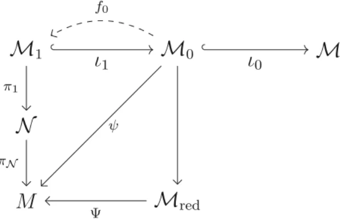
The model ˆM ofMredwas obtained by explicitly constructing a global cross section of the gauge orbits in M0. The construction of the new model M that we achieve in this paper is somewhat more complicated. We here collect the main concepts that will appear in the construction, hoping that this will enhance readability. While perusing this section, the reader is recommended to keep an eye on Fig.2presented below.

We shall describe the quotient Mred (2.34) by exhibiting a new set of unique representatives for each orbit of the ‘gauge group’K+(σ)×K+ acting onM0. We now displayMredas

Mred=K₊(σ)\M0/K₊, (3.1)

emphasizing that (η_L, η_R)∈K₊(σ)×K₊ acts by left- and by right-multipli- cation, respectively. We shall arrange taking the quotient into convenient con- secutive steps, using in addition to the obvious direct product structure of the

M

M

M N

M M

ι

ι

π1

ψ f0

π_N

Ψ

Figure 2. Construction of the modelM ofMred. The verti- cal arrows andψdenote bundle projections;ι1andι0are em- beddings. The setsM0,M1 andN are, respectively, defined in (2.32), (3.6) and (3.7). The arrow f0 represents a locally well-defined gauge transformation (3.26) depending smoothly on M0. The map π₁ is given by (3.7) and (3.8). The map π_N denotes the realization of the quotient (3.25) provided by Proposition6.4and Theorem6.5

gauge group also the fact thatK₊(σ) itself can be decomposed as the direct product

K₊(σ) =K₊( ˆw)×T1, (3.2) where

T1 ={ˆγ:= diag(γ1n, γ⁻¹1n)|γ∈U(1)}, (3.3) K+( ˆw) ={κ∈K+|κwˆ= ˆw} with ˆw= (ˆv,0)^T ∈C²ⁿ, (3.4) and ˆv∈Cⁿis the fixed vector in (2.29). It is easy to check that every element of K₊(σ) can be written as a product of these two disjunct, mutually commuting subgroups.

As in [13], we callb∈B ‘quasi-diagonal’ if it has the form b=

e^−v1n β 0 e^v1n

withβ = diag(β1, . . . , βn), β1≥β2≥ · · · ≥βn ≥0, (3.5) and define the subsetM1 of the ‘constraint surface’M0⊂ Mby

M1:={g=kb∈ M0|bis quasi-diagonal}. (3.6) The ‘left-handed’ gauge transformations byK+(σ) mapM1 to itself and by using this we introduce the quotient

N :=K₊( ˆw)\M1. (3.7)

It will be useful to identifyN with the image of the map

M1g=kb→(w(k), L(k), β) withw(k) :=k⁻¹w,ˆ L(k) :=k⁻¹IkI.

(3.8) Such an identification is possible since (w(k), L(k)) = (w(k), L(k)) fork, k ∈ K if and only if kk⁻¹ ∈ K+( ˆw). Directly from the definitions, we have K+(σ)\M1=T1\N, where ˆγ∈T1 (3.3) acts according to w(ˆγk) =γ⁻¹w(k), because of the form of ˆwin (3.4), whileL(k) andβ are unchanged.

The gauge transformation (2.28) by (ηL, ηR)∈K+(σ)×K+ acts on the kandbcomponents of g=kb∈ M0 by

(k, b)→(ηLkη_R⁻¹, ηRbη⁻¹_R ), (3.9) and thus operate on the constituentχ (2.31) ofbaccording to

χ→ηR(1)χηR(2)⁻¹, (3.10)

where we employ the block-matrix notation ηR=

ηR(1) 0 0 ηR(2)

, ηR(1), ηR(2)∈U(n), det(ηR(1)ηR(2)) = 1.

(3.11) Recalling the singular value decomposition ofn×nmatrices, we observe from (3.10) that every elementg∈ M0can be gauge transformed intoM1, and the componentsβi of the resulting element ofM1 are uniquely determined byg.

To proceed further, we restrict ourselves to the ‘regular part’ defined by the strict inequalities

β1> β2>· · ·> βn>0. (3.12) We call suchβ and the corresponding quasi-diagonalbregular, and apply the notationsM^reg₁ , M^reg₀ ,N^reg and M^reg_redfor the corresponding subsets. Specif- ically, M^reg₀ consists of the elements of M0 that can be gauge transformed intoM^reg₁ ,N^reg=K+( ˆw)\M^reg₁ andM^reg_red=K+(σ)\M^reg₀ /K+. Later it will emerge that in factM0=M^reg₀ .

Ifβ is regular, then the correspondingbin (3.5) is fixed by the following Abelian subgroup,Tn−1, ofK+:

Tn−1:=

δ= diag(δ1, . . . , δn, δ1, . . . , δn)|δi∈U(1), n i=1

δ²_i = 1

. (3.13) We shall also use the subgroup ofT1×Tn−1 given by

Z˜^diag_2n ={(ˆζ, ζ12n)|ζ∈Z2n}, (3.14) whereZ2n denotes the (2n)^th roots of unity and we employ the notation (3.3).

Defining

Tn:={τ = diag(τ1, . . . , τn, τ1, . . . , τn)|τi∈U(1)}, (3.15) we have the isomorphism

Tn(T1×Tn−1)/Z˜^diag_2n , (3.16) which is provided by the map

τ_i =γ⁻¹δ_i (3.17)

using the above parametrizations of the elements ofT1(3.3),Tn−1 (3.13) and Tn (3.15).

After these preparations, we come to the main points. First, we letδ ∈ Tn−1 act onM^reg₁ ×K+by

δ: (g, η)→(gδ⁻¹, δη) (3.18) and also letη_R∈K₊act by

ηR: (g, η)→(g, ηη⁻¹_R ). (3.19) Then we introduce the identification

M^reg₀ ←→(M^reg₁ ×K₊)/T_n−1 (3.20) by means of the map

(M^reg1 ×K₊)(g, η)→gη∈ M^reg0 , (3.21) which is invariant with respect to the action (3.18) ofTn−1. Since the actions ofTn−1 andK+ onM^reg₁ ×K+ commute, we have

M^reg0 /K₊ = ((M^reg1 ×K₊)/Tn−1)/K₊

= ((M^reg₁ ×K+)/K+)/Tn−1=M^reg₁ /Tn−1, (3.22) where on the right-end we refer to the action ofTn−1onM^reg1 given byM^reg1 kb → kbδ⁻¹ = kδ⁻¹b. We continue by applying the decomposition (3.2) of K₊(σ) to deduce the identification

M^reg_red= (K+( ˆw)×T1)\M^reg₁ /Tn−1=T1\N^reg/Tn−1, (3.23) where we have taken into account thatN^reg=K₊( ˆw)\M^reg1 (see (3.7)). The action ofT1×Tn−1 onN^reg factors through the homomorphism (3.17). The induced action ofTn (3.15) onN^reg is given, in terms of the triples (w, L, β) in (3.8) representing the elements ofN^reg, by the formula

(w, L, β)→(τ w, τ Lτ⁻¹, β), ∀τ∈Tn. (3.24) One sees this from the definitions in (3.8) and in (3.17) using that (ˆγ, δ) ∈ T1×Tn−1sendsg=kb∈ M^reg1 to (ˆγkδ⁻¹)b∈ M^reg1 . The final outcome is the following identification:

M^reg_red=N^reg/Tn. (3.25) The action (3.24) ofTnonN^regis actually a free action. This is a consequence of the fact [8] that the action of (K+(σ)×K+)/Z^diag_2n onM0 is free.

Remark 3.1. Every element ofM0can be mapped intoM1by a gauge trans- formation, which is unique up to residual gauge transformations acting onM1. It is a useful fact thatlocally, in a neighborhood of any fixed element ofM^reg0 , a well-defined mapf₀can be chosen,

f0:M^reg₀ g→g1∈ M^reg₁ , (3.26) in such a manner that the gauge transformed matrixg₁ depends analytically on the local coordinates on the manifoldM^reg0 . We next explain this statement.