,S´andorFrey andKrisztina´E.Gab´anyi EmmaKun Aself-lensingsupermassivebinaryblackholeatradiofrequencies:thestoryofSpikeycontinues

arXiv:2006.08441v1 [astro-ph.HE] 15 Jun 2020

A self-lensing supermassive binary black hole at radio frequencies: the story of Spikey continues

Emma Kun

, S´ andor Frey

and Krisztina ´ E. Gab´ anyi

1Konkoly Observatory, Research Centre for Astronomy and Earth Sciences, Konkoly Thege Mikl´os ´ut 15-17, H-1121 Budapest, Hungary 2Institute of Physics, ELTE E¨otv¨os Lor´and University, P´azm´any P´eter s´et´any 1/A, H-1117 Budapest, Hungary

3Department of Astronomy, E¨otv¨os Lor´and University, P´azm´any P´eter s´et´any 1/A, H-1117 Budapest, Hungary 4MTA-ELTE Extragalactic Astrophysics Research Group, P´azm´any P´eter s´et´any 1/A, H-1117 Budapest, Hungary

ABSTRACT

The quasar J1918+4937 was recently suggested to harbour a milliparsec-separation binary supermassive black hole (SMBH), based upon modeling the narrow spike in its high-cadenceKepleroptical light curve. Known binary SMBHs are extremely rare, and the tight constraints on the physical and geometric parameters of this object are unique. The high-resolution radio images of J1918+4937 obtained with very long baseline interferometry (VLBI) indicate a rich one-sided jet structure extending to 80 milliarcseconds. Here we analyse simultaneously-made sensitive 1.7- and 5-GHz archive VLBI images as well as snapshot 8.4/8.7-GHz VLBI images of J1918+4937, and show that the appearance of the wiggled jet is consistent with the binary scenario.

We develop a jet structural model that handles eccentric orbits. By applying this model to the measured VLBI component positions, we constrain the inclination of the radio jet, as well as the spin angle of the jet emitter SMBH. We find the jet morphological model is consistent with the optical and radio data, and that the secondary SMBH is most likely the jetted one in the system. Furthermore, the decade-long 15-GHz radio flux density monitoring data available for J1918+4937 are compatible with a gradual overall decrease in the the total flux density caused by a slow secular change of the jet inclination due to the spin–orbit precession. J1918+4937 could be an efficient high-energy neutrino source if the horizon of the secondary SMBH is rapidly rotating.

Key words: galaxies: active – galaxies: jets – radio continuum: galaxies – quasars:

supermassive black holes – quasars: individual: J1918+4937

1 INTRODUCTION

RecentlyHu et al. (2020) interpreted a narrow spike in the densely-sampled Kepler optical light curve of the quasar J1918+4937 (also known as KIC 11606854, dubbed as Spikey by Hu et al. 2020) as a result of gravitational self- lensing in a supermassive black hole binary (SMBHB) sys- tem. The quasar has a spectroscopic redshift of z_sp=0.926 (Healey et al. 2008). In this scenario, the orbital plane of the binary lies sufficiently close to the line of sight so that when one of the companions – the black hole with the larger mass – passes in front of the other, the optical emission of the lat- ter active galactic nucleus (AGN) is significantly enhanced.

Taking two relativistic effects, the binary self-lensing and the orbital Doppler boosting into account,Hu et al. (2020) modeled theKepler light curve containing the spike. They found that the system is composed of two black holes (BHs),

⋆ Email: kun.emma@csfk.mta.hu

with masses of2.5×10⁷ M_⊙and5.0×10⁶M_⊙. The eccentric orbit (e≈0.52) has a period ofT =418d in the rest frame of the object. From our point of view, the orbital plane is seen almost edge-on, within an angle of∼8^◦.

Studying binary AGNs is an active field of both ob- servational and theoretical astrophysics, due to its con- nection to cosmological structure formation, galaxy evolu- tion, and most recently gravitational waves. Observations of such objects are very challenging (for a review see e.g.

Komossa & Zensus 2016), and securely confirmed cases are extremely rare (De Rosa et al. 2019). Spikey stands out from the very few SMBHB candidates because the binary self- lensing model (Hu et al. 2020) constrains the orbital param- eters, the geometry, and the masses of the companions very accurately. The model also provides a testable prediction that the next flaring will occur in 2020.

Apart from being a moderately bright X-ray AGN (Hu et al. 2020), J1918+4937 is also a prominent radio-loud quasar. Variations in its ∼ 100-mJy level flux density at

©

15 GHz are being monitored at the Owens Valley Radio Observatory (OVRO, Richards et al. 2011). The source is known to have a compact radio jet structure at milliarcsec (mas) angular scales, as revealed by very long baseline inter- ferometry (VLBI) imaging observations (e.g. Kovalev et al.

2007). Detecting binary AGNs separated by a small fraction of a pc is practically impossible with direct imaging obser- vations, even with the high resolution offered by VLBI and in the most nearby universe (e.g. An et al. 2018). But ra- dio interferometric observations could help in another way, by detecting a discernible effect of a binary companion on the appearance of the relativistic jet produced by the other AGN in the system, because the orbital motion of the jetted AGN may result in a helical shape of the jet (for a recent review, seeDe Rosa et al. 2019, and references therein).

A growing number of studies propose radio-loud AGNs as strong candidates for efficient high-energy (HE) neutrino emitter objects, especially the blazars (e.g. Kadler et al.

2016; IceCube Collaboration et al. 2018a; Garrappa et al.

2019;Giommi et al. 2020), whose jets point close to the line of sight of the observer. The underlying physical mechanisms involve light–matter and/or matter–matter interactions in a relativistically moving plasma.Kun et al.(2017,2019) pro- posed a model in which the radio and neutrino observations were put into a common physical picture involving the spin- flip of a SMBH in a merging binary. Recently theγ-ray flar- ing blazar TXS 0506+056, an efficient particle accelerator, turned out to be the source of several IceCube neutrinos (IceCube Collaboration et al. 2018a;IceCube Collaboration 2018b). Studies indicate that neutrino emission might be due to a recent merger activity (Britzen et al. 2019; Kun et al.

2019). Although there is no indication yet of an observed neutrino event near its position, Spikey is a VLBI source directing its jet close to our line of sight, and also a SMBH binary candidate, making this AGN an object of great in- terest as a potential neutrino source.

In this paper, we investigate whether the available ra- dio data are consistent with the behaviour of the object, the gravitational self-lensing model, and in particular the pa- rameters derived for Spikey by Hu et al. (2020). Based on archival data from 2008, we present sensitive and detailed VLBI images of J1918+4937 obtained at 1.7 and 5 GHz for the first time, and show the OVRO flux density curve (Sect.2). By modeling the source brightness distribution at

∼1−10mas scale, we derive parameters describing the rela- tivistic jet, estimate the apparent speed of the jet based on snapshot VLBI observations conducted at the 8.4/8.7 GHz frequency band, and put forward a scenario where a jet is launched from one of the accreting BH components of the system in Sect.3. Here we also investigate the case whether the OVRO flux density curve is compatible with the binary model. We discuss our findings based on the OVRO single- dish and VLBI radio observations in Sect.4. We also discuss whether Spikey could be an efficient high-energy neutrino emitter in the near future based on the behaviour of its VLBI jet and the proposed SMBH merger scenario. Finally we conclude the paper with a summary in Sect.5.

We assume a flat ΛCDM cosmological model with H₀=70 km s⁻¹ Mpc⁻¹,Ωm =0.3, andΩ_Λ =0.7in this pa- per. In this model, an object atz_sp=0.926has a luminosity distance ofD_L≈6Gpc, and 1 mas angular size corresponds to7.853pc projected linear size (Wright 2006).

2 RADIO OBSERVATIONS

2.1 VLBI imaging observations and data reduction

Kharb et al. (2010) studied the Seyfert galaxy NGC 6764 with high-resolution VLBI imaging at 1.7 and 5 GHz.

The observations were conducted with the U.S. Very Long Baseline Array (VLBA) in phase-referencing mode (Beasley & Conway 1995) where J1918+4937 (1917+495) was selected as the nearby compact calibrator source within 2^◦ separation from the target. Nine 25-m diameter antennas of the VLBA (Brewster, Fort Davis, Hancock, Kitt Peak, Los Alamos, Mauna Kea, North Liberty, Owens Valley, and Pie Town) participated in the experiment BK154, performed on 2008 November 13-14 with a total duration of about 14 h.

The observations at both frequencies were made with two 8-MHz wide intermediate frequency channels (IFs) in both left and right circular polarizations. The total bandwidth was therefore 32 MHz.

Kharb et al. (2010) scheduled the observations in 5- min switching cycles, with 2 min spent on the calibrator J1918+4937 and 3 min on the weak target NGC 6764, in- cluding antenna slewing times. As a valuable byproduct of this phase-referencing experiment,∼1.6 and 1.8 h of VLBA data accumulated on our object of interest, J1918+4937, at 1.7 and 5 GHz, respectively.

We downloaded the raw VLBA data of the BK154 ex- periment from the public archive¹of the U.S. National Radio Astronomy Observatory (NRAO). For the data calibration, we used the NRAO Astronomical Image Processing Sys- tem (AIPS,Greisen 2003) in a standard way (e.g.Diamond 1995). We started with calibrating the ionospheric delays based on total electron content measurements, and corrected for the measured Earth orientation parameters. We applied digital sampler corrections, then used a short 1-min scan on the bright fringe-finder source 1758+388 to solve for in- strumental phases and delays. Bandpass correction was per- formed using the same scan. We used the gain curve and sys- tem temperature information from the participating VLBA stations for a-priori amplitude corrections. Finally fringe- fitting was done and the solutions were applied to the data.

The calibrated visibility data of J1918+4937 were ex- ported to theDifmapsoftware (Shepherd et al. 1994). Af- ter the standard hybrid mapping procedure involving sev- eral iterations of clean decomposition, phase-only self- calibration, and finally phase and amplitude self-calibration, we obtained the naturally-weighted 1.7- and 5-GHz VLBI images of J1918+4937 shown in Fig. 1. As a finishing step of data reduction, we fitted circular Gaussian brightness dis- tribution model components directly to the self-calibrated visibility data inDifmap. This allows us to describe the ra- dio structure with a limited set of parameters that are listed in Table1, where the errors were calculated as inKun et al.

(2014). These model components will be used for determin- ing the shape of the jet. This way we can also gain informa- tion on the Doppler boosting of the relativistic jet.

Further VLBI imaging observations of J1918+4937 made at the 8.4/8.7-GHz frequency band are available in

1 https://archive.nrao.edu

Figure 1.VLBA images of J1918+4937.Left:at 1.7 GHz. The peak intensity is 128 mJy beam⁻¹. The lowest contours are drawn at

±0.3mJy beam⁻¹. The elliptical Gaussian restoring beam is 8.9 mas×6.4 mas (FWHM) at a position angle−28^◦.Right:at 5 GHz. The peak intensity is 119 mJy beam⁻¹. The lowest contours are drawn at±0.28mJy beam⁻¹. The restoring beam is 2.9 mas×2.1 mas (FWHM) at a position angle−38^◦. In both images, the positive contour levels increase by a factor of 2, and the restoring beam size is indicated in the bottom-left corner.

Table 1.Parameters of the circular Gaussian model components fitted to the 1.7 and 5 GHz VLBI visibility data of J1918+4937.

Frequency Flux density Relative position Diameter (GHz) F (mJy) R.A. (mas) Dec. (mas) FWHM (mas)

1.7 104±6 0.00±0.34 0.00±0.41 0.57±0.01 30±2 −2.07±0.36 2.56±0.42 1.18±0.01 24±2 −6.03±0.39 5.29±0.45 2.02±0.01 7±1 −9.07±0.38 9.23±0.44 1.73±0.01 5±1 −14.36±0.46 16.51±0.51 3.17±0.08 4±1 −21.76±0.97 23.79±0.99 9.08±0.15 5±2 −34.95±1.71 40.20±1.73 16.80±2.73 5 100±7 0.00±0.12 0.00±0.13 0.18±0.01

32±4 −0.81±0.12 1.09±0.13 0.33±0.01 6±2 −2.70±0.18 3.43±0.19 1.39±0.02 6±1 −4.85±0.20 4.90±0.20 1.59±0.05 4±1 −7.26±0.17 6.06±0.17 1.17±0.02 3±1 −8.43±0.28 8.28±0.28 2.54±0.03 3±1 −13.45±0.70 16.71±0.70 6.86±0.71

the Astrogeo data base² covering a13-yr long interval from 2005 to 2018. These are short snapshot VLBA observations of varying quality, typically with scans of few minutes, not suitable for recovering the fine details of the jet structure.

We downloaded the calibrated visibility data and performed imaging and model fitting in Difmap. At each epoch, we could at least model the core emission and the innermost jet component with circular Gaussian brightness distribu- tion components, allowing us to measure their angular sep- aration. The values are given in Table 2 and plotted as a function of time in Fig.2. We also included here the 5-GHz data point (Table1) because it was obtained at a close fre- quency and it helps filling the gap in the time coverage of the 8.4/8.7-GHz measurements. Although the data points have a scatter beyond the formal uncertainties due to the compli- cations with imaging a complex structure from limited ob- servations, the component separation clearly increases with

2 http://astrogeo.org/cgi-bin/imdb get source.csh?source=J1918%2B4937

Table 2.Separation of the core and the innermost jet component measured at 8.4/8.7 GHz and 5 GHz.

Date Frequency Separation

(GHz) (mas)

2005 Jul 09 8.6 1.06±0.03 2008 Nov 13 5.0 1.35±0.02 2012 Feb 20 8.4 1.48±0.04 2012 Mar 09 8.4 1.14±0.14 2014 Aug 06 8.7 2.26±0.03 2017 Jul 09 8.7 2.42±0.04 2018 Jul 01 8.7 2.35±0.02

time. The line in Fig.2indicates the linear fit for estimating the apparent angular proper motion,0.10±0.01mas yr⁻¹.

0.8 1 1.2 1.4 1.6 1.8 2 2.2 2.4 2.6

2004 2006 2008 2010 2012 2014 2016 2018 2020

Core separation (mas)

Time (yr) linear fit

5 GHz 8.4/8.7 GHz

Figure 2. Separation of the core and the inner jet component identified at each epoch in J1918+4937 as a function of time, based on 8.4/8.7-GHz (filled circles) and 5-GHz (open triangle) VLBI measurements. The line represents the linear fit for esti- mating the apparent angular proper motion,0.11±0.01mas yr⁻¹.

2.2 Total flux density monitoring

The quasar J1918+4937 is included in the sample of extra- galactic sources regularly monitored with the 40-m OVRO radio telescope at 15 GHz frequency (Richards et al. 2011).

The total flux density variability of J1918+4937 from early 2008 to date can be seen in Fig.3which we constructed from the monitoring data available at the OVRO website³. A few flux density data points (∼ 9% of the total number) with excessively large error bars were discarded as unreliable.

The data after 2015 November 28 (2015.9) have error bars typically a factor of ∼ 2smaller than before. This is likely due to the new receiver installed at OVRO in 2014 June, and a new data processing pipeline used. Keeping in mind that the time sampling of the flux density curve is more or less uniform, we re-scaled the error bars, in order to associate comparable weights to the older and the more recent data for a subsequent model fitting. The procedure was as follows. For the n-th data point, we calculated the standard deviation of the flux densities in the range [(n− k). . .(n+k)]with k =10, and assigned it to then-th data point as its new error bar. This way, the first and lastkdata points had to be dropped from the light curve. The 15-GHz flux densities with the smoothed error bars are shown in Fig.3, overlaid on the original light curve.

3 RESULTS 3.1 Jet parameters

Figure1shows an asymmetric radio structure with a com- pact core and a one-sided extension. It is typical for bright radio-loud quasars where the emission from one of the in- trinsically symmetric jets that is pointing close to the ob- server’s line of sight is enhanced by relativistic beaming (for a recent review, see Blandford et al. 2019). In the case of J1918+4937, the approaching jet is pointing towards the Northwest as projected on the sky. The radio emission can

3 http://www.astro.caltech.edu/ovroblazars/

be traced out to about 80 mas at the lower observing fre- quency, 1.7 GHz, then it becomes diffuse and resolved out on the long interferometer baselines. This angular extent corresponds to a projected linear size of 630 pc.

The bright VLBI core at the southeastern end of the nearly straight structure (Fig.1) is in fact the base of jet where it becomes optically thick at the given observing fre- quency. The fitted Gaussian model parameters of the core (Table1) can be used to calculate the apparent brightness temperature,

T_b=1.22×10¹² F

θ²ν²(1+z_sp)K, (1)

whereFis the flux density measured in Jy,θthe diameter of the circular Gaussian component in mas (full width at half- maximum, FWHM), andνthe observing frequency in GHz.

Taking into account the redshift of J1918+4937,z_sp=0.926, the core brightness temperatures are(2.6±0.4) ×10¹¹K and (2.9±0.2) ×10¹¹ K at 1.7 and 5 GHz, respectively. These values agree within their uncertainties, so we adopt T_b ≈ 2.7×10¹¹K for the further calculations.

The ratio between the apparent and the intrinsic bright- ness temperatures gives the Doppler-boosting factor, δ = T_b/T_b,int. If we follow the usual practice and assume the equipartition brightness temperature (Readhead 1994) as T_b,int≈5×10¹⁰ K, then the Doppler factor isδ≈5. On the other hand, based on measurements of a sample of pc-scale jets,Homan et al.(2006) arrived at a somewhat lower typi- cal intrinsic brightness temperature value,T_b,int≈3×10¹⁰K.

Considering this, the Doppler factor of the jet in J1918+4937 would becomeδ≈9.

The amount of Doppler boosting depends on two fun- damental jet parameters, the bulk Lorentz factor (Γ) of the plasma flow (i.e. the intrinsic jet speed) and the jet incli- nation with respect to the line of sight (ι₀). If the appar- ent proper motion of the jet components can be measured based on VLBI imaging observations conducted at multiple epochs, it is possible to estimate values ofΓ andι₀ as well (e.g.Urry & Padovani 1995). Even though sensitive imaging data are found in the archives for J1918+4937 at a single epoch only at the above frequencies (1.7 and 5 GHz), from the available multi-epoch snapshot 8-GHz VLBI observa- tions we were able to track the motion of one of the inner jet components. Assuming a linear outward motion (Fig.2), we estimate its apparent speed in the units of the speed of light (c) asβ_app=5.33±0.65. If we considerβ_appas a repre- sentative estimate of the apparent jet speed in J1918+4937, and take the possible values of the Doppler factors derived above, we can obtain (see e.g.Urry & Padovani 1995) the bulk Lorentz factor

Γ=

β²_app+δ²+1

2δ (2)

and the jet inclination angle cosι₀= Γ−δ⁻¹

√Γ²−1

. (3)

Forδ=5, we getΓ≈5.4andι₀≈11.^◦5, and forδ=9, we get Γ≈6.1andι₀≈5.^◦6.

t

t

t

2008 2010 2012 2014 2016 2018 2020

40 60 80 100 120 140 160 180

Time(yr)

15GHzfluxdensity(mJy)

Figure 3.The OVRO single-dish flux density curve of Spikey at 15 GHz. The original measurement points with error bars are shown in green, overlaid by the smoothed data (i.e. the data points with re-scaled error bars) in black. The best-fit linearly decreasing trend is indicated by the red line (see Sect.3.4). The labelstA(at 2008.222) andtC(at 2019.222) mark the first and last epochs of the smoothed flux density curve, whiletBmarks the epoch of the 1.7- and 5-GHz VLBI observations (2008.870).

3.2 Jet structural model utilizing eccentric SMBH orbit

While the jet shape in Fig. 1 seems remarkably straight on scales of several tens of mas, some wiggling is also ap- parent, especially at 5 GHz where the angular resolution is higher. Here we build up a structural (morphological) model of the jet as seen projected onto the plane of the sky, based on the fitted circular Gaussian model component positions (Table1). We assume that these compact radio components were launched by a jetted supermassive black hole (SMBH) moving along an eccentric orbit in the binary system, and the jet launching is affected by the periodically changing orbital velocity of the jet emitter SMBH. This idea was ap- plied earlier in several studies (Roos et al. 1993;Kun et al.

2014,2015) but for circular orbits. Here we further develop the model, to allow for eccentric binary orbits with arbitrary spin angles. Note that in the jet model below, the jet com- ponents themselves move along ballistic trajectories and not along helical paths. Rather we see a helical pattern on the sky formed by the subsequently emitted components, as the angle of the jet launching changes periodically. We assume that this pattern motion preserves the jet launching angle at least up to tens of mas from the central engine. Meanwhile, the physical distances between the components are growing as the time passes.

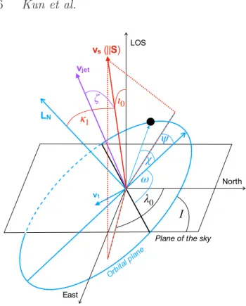
Let us assume an orthogonal coordinate system K in which thezaxis is parallel to the orbital angular momentum L_N=L_NLˆ_N(z||Lˆ_N) (hereLˆ_Ndenotes the unit vector pointing to the direction of the orbital angular momentum), and the x axis is directed towards the pericentre of the orbit. The orbital configuration is depicted in Fig.4. The instantaneous orbital velocity vector of thei-th BH in the orbital plane as a function of the eccentric anomalyE is

v_i(E)= v_i,x(E)

v_i,y(E)

=v_0,i

−sinχ(E) e+cosχ(E)

, (4)

where v_0,i is the circular orbital speed of the jet emitter SMBH (i=1for the dominant, andi=2for the secondary- mass BH),

χ(E)=2 arctan

"r 1+e 1−etanE

2

#

(5)

is its true anomaly, a=

G(m₁+m₂) 4π²

T² 1/3

(6) is the semi-major axis of the orbit, G is the gravitational constant,T is the orbital period, m =m₁+m₂ is the total mass, and eis the orbital eccentricity. If the dominant BH is the jet emitter, then its velocity should be considered in Eq.4, which is

v_0,1=2π T

a

√1−e² m₂

m₁+m₂, (7)

and if the secondary BH is the jetted one, its velocity is v_0,2=2π

T p a

(1−e²) m₁

m₁+m₂. (8)

The direction of the jetted BH spinS_i inK is the unit vector

ˆS_i=(sinκ_icosψ_i,sinκ_isinψ,cosκ_i), (9) whereκ_i =arccos(ˆS_i·Lˆ_N)is the angle betweenS_iand the or- bital angular momentumL_N, andψ_iis the angle between the projection of the spin onto the orbital(x,y)plane and the pe- riapsis line. We assume that one of the two BHs emits the jet via the Blandford–Znajek mechanism (Blandford & Znajek 1977). In this case, the jet symmetry axis is directed along the BH spin S_i, consequently the unperturbed jet velocity vector becomesv_s=vsˆS_i inK, and its components are v_s=©­

« vs,x

v_s,y vs,z

ª®

¬

=©­

«

vssinκ_icosψ_i v_ssinκ_isinψ_i

vscosκ_i ª®

¬

. (10)

The jet velocity vectorv_jet is the vectorial sum of the un- perturbed jet velocity vectorv_s and the orbital velocityv_i, such that

v_jet=©­

« vjet,x

v_jet,y vjet,z

ª®

¬

=©­

«

vssinκ_icosψ_i−v_0,isinχ v_ssinκ_isinψ_i+v_0,i(e+cosχ)

vscosκ_i

ª®

¬

. (11)

Letζ be the angle betweenv_jetand v_s, which is calcu- lated as

sinζ=|v_jet×v_s|

|v_jet||v_s|, (12)

vs(||S)

LN

vjet

κ

χ ψ

ω λ

ι

ζ

v1

LOS

North

East

Plane of the sky

Orb ital plane

I

Figure 4.Geometric configuration of the Spikey system centred on its barycentre. The black dot marks the position of the jet- emitting SMBH along its elliptical orbit. LOS indicates the line of sight, andL_Nis the Newtonian orbital angular momentum. The true anomaly isχ, the argument of the periapsis isω, the orbital inclination is I, the BH spin angle with respect to the orbital normal isκ1, the angle between the projection of the spin onto the orbital plane and the periapsis line isψ, and the inclination angle of the spin with respect to the LOS isι0. The position angle of the spin projected onto the plane of the sky (λ0) is measured from North through East. Furthermore,v1is the orbital velocity vector of the jet-emitting SMBH at the instant of the jet component launching (if the secondary BH emits the jet, for its argument of periapsisω2=ω1+πholds in radians), vsis the original jet velocity vector (that is parallel to the spin) andvjetis the vectorial sum of the above two. Finally,ζis the instantaneous half-opening angle of the jet. For the sake of clarity, we shifted the jet velocity vector to the barycentre. In reality, the jet launches from the immediate vicinity of the emitting SMBH.

where

|v_jet×v_s|=v_0,ivscosκ_i q

C₁+C₂tan²κ_i (13) with

C₁=1+e²+2ecosχ, C₂=(cos(χ−ψ_i)+ecosψ_i)², and

|v_jet||vs|=vsp

C₃+C₄+C₅ (14)

with

C₃=v²_scosκ_i²,

C₄=(v_0,isinχ−vscosψ_isinκ_i)², C₅=(v_0,i(e+cosχ)+vssinκ_isinψ_i)².

For the orbital velocities in Spikey, even at this sub-pc separation,v_0,i ≪v_s, and then the series expansion of their ratio (Eq.12) in leading order gives

sinζ=v_0,icosκ_i v_s ×

× q

1+e²+2ecosχ+(cos(χ−ψ_i)+ecosψ_i)²tan²κ_i. (15) Now let us define a new orthogonal coordinate system K^′, such that itsz′axis is parallel to the spin of the jetted BH. In this system, the jet morphological model turns to x^′(u)=

B

2πu[−sinχ(u−φ)], (16)

y^′(u)= B

2πu[e+cosχ(u−φ)], (17) z^′(u)=

A

2πu, (18)

whereuis the polar angle (Kun et al. 2014),φis the initial phase of u, and B is the jet growth in mas perpendicular to its symmetry axis whileu changes by 2π over the time periodT_u. This latter quantity is measured in the observer’s frame as

B^′=v_0,icosκ_iT_u

s (1+z_sp), (19)

where v_0,icosκ_i is the orbital velocity perpendicular toS_i, sis the scale factor that relates projected linear size to the measured angular size (in pc mas⁻¹). Another parameter,A is the jet growth in mas parallel to its symmetry axis while uchanges by2πover the time periodT_u. The quantity Ais measured in the observer’s frame as

A^′=

v_jet+v_0,i q

1+e²+2ecosχ(u−φ)cosκ_i T_u

s (1+z_sp). (20) Then we define a coordinate systemK^′′, such that the x′′

andy^′′axes point to East and North in the plane of the sky, respectively, and thez′′axis coincides with the direction of the line of sight (LOS), as shown in Fig. 4. The inclina- tion angle between the LOS and the spin of the jet emitter BH is ι₀ (which we call spin inclination angle), and λ₀ is its position angle measured from North (y^′′ axis) through East (x^′′axis). Employing the same rotational matrices as inKun et al.(2014),

x^′′(u)=

x^′(u)cosι₀+z^′(u)sinι₀

cosλ₀−y^′(u)sinλ₀, (21) y^′′(u)=

x^′(u)cosι₀+z^′(u)sinι₀

sinλ₀+y^′(u)cosλ₀. (22) In this model, the helical jet shape is in fact the pattern drawn by the perturbed jet components ejected at different epochs from the central engine. In other words, the individ- ual components do not move along a helix, rather the pattern they collectively form grows both in the direction of the spin and perpendicular to it, as described by the parameters A andB, respectively.

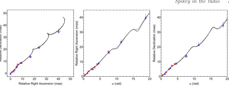
3.3 Application of the jet model to the VLBI data After setting up the model to describe the jet structure, we now take into account the measured VLBI component posi- tions at 1.7 and 5 GHz (Table1) and derive the model pa- rameters. These observations were made at the same time,

■■■■■

■

▲▲

▲ ▲

▲

▲

▲

0 10 20 30 40 50

0 10 20 30 40 50

Relative Right Ascension(mas)

RelativeDeclination(mas)

■■ ■■■

■

▲▲ ▲

▲

▲

▲

▲

0 5 10 15 20

0 10 20 30 40

u(rad)

RelativeRightAscension(mas)

■■■■■

■

▲▲

▲ ▲

▲

▲

▲

0 5 10 15 20

0 10 20 30 40

u(rad)

RelativeDeclination(mas)

Figure 5.The modeled jet shape fitted to the 1.7- and 5-GHz VLBI component positions, marked by blue triangles and red squares, respectively.Left:the right ascension and declination of the components relative to the VLBI core and the best-fit jet shape assuming Doppler factorδ=5, once with the dominant-mass (m1) SMBH being the jet emitter (dotted black curve) and then with the secondary- mass (m2) SMBH (continuous black curve).Middle:the right ascension of the components relative to the VLBI core as a function ofu.

Right:the declination of the components relative to the VLBI core as a function ofu. The jet structure is rotated by90^◦towards East.

Table 3.Grid parameters of the best-fit models, such as projected pitch along the spin (A^′′), Lorentz factor (Γ), spin angle (κ), and those derived from them, the spin inclination angle (ι0) and the jet speedβ, assuming that either the dominant-mass SMBH(top)or the secondary SMBH(bottom)launches the jet. We show the lowestχ-square values (χ_min² ). We also list the parameter ranges in which the models are indistinguishable from each other (i.e.∆AIC≤2) and give the averages and standard deviations of the parameters in those ranges.

The jet is emitted by the larger mass SMBH (m1) δ=5(χ_min² =34.54) δ=9(χ_min² =33.84)

∆AIC≤2 ∆AIC≤2

A^′′(mas) [16.6:19.3] 17.9±0.6 [16.7:19.1] 17.9±0.6 Γ [3.0:20.0] 16.2±4.9 [5.0:20.0] 12.7±4.2 κ(^◦) [0:30] 11.0±7.5 [0:64] 23.5±13.2 ι0(^◦) [7.6:8.8] 8.0±0.3 [3.7:6.4] 5.9±0.4 β(c) [0.943:0.999] 0.992±0.017 [0.980:0.999] 0.992±0.008

The jet is emitted the smaller mass SMBH (m2) δ=5(χ_min² =31.42) δ=9(χ_min² =31.85)

∆AIC≤2 ∆AIC≤2

A^′′(mas) [16.7:19.1] 17.9±0.6 [16.7:19.1] 17.9±0.6 Γ [3.0:20.0] 10.6±4.9 [5.0:20.0] 12.4±4.3 κ(^◦) [65:79] 73.0±3.0 [77:85] 79.8±1.4 ι0(^◦) [7.6:11.5] 9.7±1.3 [3.7:6.4] 5.9±0.5 β(c) [0.943:0.999] 0.990±0.012 [0.980:0.999] 0.995±0.004

but at different frequencies, and the position of the opti- cally thick core components (i.e., the base of the jet used as a reference for the relative position of other components further along the jet) is known to depend on the observing frequency, an effect called core shift (Blandford & K¨onigl 1979;Lobanov 1998).Sokolovsky et al. (2011) conducted a dedicated survey with the VLBA at nine frequencies in the 1.4−15.4GHz range to quantify the core-shift effect in20 AGN jets. The average (and median) core shift between1.7 and 5 GHz was found to be approximately 0.9 mas. This is comparable to the uncertainties of our component posi- tions (Table 1). Therefore we used model components fit- ted at both 1.7 and 5 GHz together in the further analy-

sis. Note that the angular resolution of the interferometer is about 3 times better at the higher frequency. Thus the inner section of the jet is characterised by more components at 5 GHz, while the outer section is only seen at 1.7 GHz, where the array is more sensitive to the weaker, extended, steep-spectrum features.

We are in a unique situation because some of the key parameters of the Spikey SMBHB system are accurately known fromHu et al.(2020). Therefore we adopt the (rest- frame) orbital periodT =1.14yr, the orbital inclination I= 1.43rad, the mass of the primary SMBHm₁=2.5×10⁷M_⊙, the mass of the secondary SMBH m₂ = 5.0×10⁶M_⊙, and the orbital eccentricity e = 0.52. These numbers imply

a = 5.1×10¹³m = 0.002 pc and the circular velocities v_0,1≈0.006candv_0,2≈0.03c. The bulk jet speed (expressed in the units ofc) and the spin inclination angle with respect to the LOS are

βs= r

1− 1

Γ² (23)

and ι₀=arccos

1 βs

1− 1

Γδ

, (24)

respectively (e.g.Urry & Padovani 1995), whereβs=vs/c. We apply non-linear least squares curve (paramet- ric) fitting with σ⁻² weights by employing the Levenberg–

Marquardt algorithm to get the best-fit jet model, such that the χ² was minimized during the process. As a next step, we characterise the reliability of our best-fit model and in- vestigate whether there are other solutions that cannot be discriminated from the above one, solely based on their χ² value. The Akaike information criterion (AIC, Akaike 1974) estimates the quality of each model relative to each of the others, i.e. it is a tool for model selection, either for nested or not nested models. The lower the AIC, the better the perfor- mance of the given model. Models in which the difference in AIC relative toAIC_minis≤2perform approximately equally (Burnham & Anderson 2002), therefore the selection of any of them might lead to inconclusive statements. Here, as the number of parameters is the same, we select the models of approximately equal quality solely based on their χ²values.

If we apply the Doppler factor δ = 5 (see Sect. 3.1), then a lower limit for the Lorentz factor isΓmin=2.6. This corresponds to the case when the jet is seen exactly pole- on (i.e. ι₀ =0). For a numerical parameter estimation, we set up a grid where the projected jet growth along the spin direction,A^′′=A^′sinι₀changes from10to30mas (in steps of∆A′′=0.1mas),Γchanges from3to20(in steps of∆Γ= 0.5), and κ_i changes from 1^◦ to 90^◦ (in steps of ∆κi =1^◦).

The bulk jet speed varies from 0.9428c to 0.9987c on the grid asΓchanges between3and20. The only parameter we have to solve for isφ_i, whileA^′′,Γ, andκ_iare changing along the grid as described above. Sincev_0,i ≪vjet, we neglect the term corresponding tov_0,i in A^′(Eq.20), and the jet grows along the spin direction solely as a result of the non-zero jet velocityv_jet.

By fitting the jet model described by Eqs. 21-22, the following best-fit parameters emerged if we assume the dominant-mass BH as the jetted one: A^′′ =17.9mas, Γ = 20.0,κ₁=0^◦(with the lowestχ²=34.54, reducedχ_R² =1.38).

The modeled jet shape corresponding to these values and the measured VLBI component positions are plotted in Fig.5.

After considering the best-quality models leading toAICdif- ference fromAIC_min as∆AIC≤2, we calculate the average value and the standard deviation of the grid parameters.

We repeated the process with Doppler factor δ = 9 (cor- responding to T_b,int = 3×10¹⁰ K; see Sect.3.1). Selecting the best-quality models, we get again the average value and the standard deviation of their grid parameters. The best- fit grid parameters, as well as parameters of models giving the same performance are summarized in Table3for δ=5 and δ = 9. We also show here the spin inclination angles (ι₀) and jet speeds (β) derived from the corresponding grid parameters. It seems that the model is not very sensitive to

the Lorentz factor, which is not surprising because the same projected jet opening angle can be generated with a variety of parameter pairs if we allow to simultaneously change the jet growth in the direction to the spin and perpendicular to it. Note that the best-fit jet structure model (χ²=34.54) is achieved withκ₁=0^◦, and the parameter range ofκ₁ giving models with comparable quality emerged as [0^◦:30^◦]. The or- bital velocity of the more massive SMBH is relatively small compared to the jet velocity along the spin because of the small BH mass ratio in Spikey. The fitting process tries to balance it with increasing thecosκi term in Eq.19in order to model the observed jet growth perpendicular to the spin as closely as possible.

We repeated the jet-shape-fitting process, now assum- ing them₂mass SMBH as the jetted one. The grid parame- ters of the best-fit jet model, the parameter ranges in which the models lead to ∆AIC ≤2, as well as the averages and standard deviations of the parameters in these ranges are summarized in Table3. The modeled jet shape correspond- ing to these values is plotted in Fig.5. If the secondary-mass SMBH is assumed as the jet emitter, then the best-fit model givesκ₂=73^◦ ifδ=5, with a slightly lower χ²=31.42com- pared to the value found for the primary SMBH. The case is similar forδ=9, and the corresponding parameter ranges leading to ∆AIC ≤ 2 are much more tightly constrained, without containing the limitingκ_i =0. This is because the velocity of the secondary SMBH is much larger compared to the more massive one, and the observed jet growth perpen- dicular to the spin can be modeled without maximizing the v_0,icosκ_i term in Eq.19.

3.4 Total flux density variations

The observed period in the optical light curve of Spikey is T_obs =(1+z_sp)T =805 d, which was recognised as the ob- served orbital period of the SMBH binary (Hu et al. 2020).

The 15-GHz radio flux density curve (Fig.3, Sect.2.2) mea- sured at OVRO (Richards et al. 2011) indicates a decreasing trend on a long term, together with some flaring activity, and possibly a longer flare started at around 2015 November. If we interpret the flux density changes as quasi-periodic, a sig- nal with500−600-d period might seem superimposed on the linear trend. This period is∼200−300d shorter than the one in the optical light curve and therefore we could not reliably fit a periodic component by employing the proposed binary parameters of Spikey (Hu et al. 2020), where the periodi- cally strengthened Doppler boosting would readily explain the radio flux density variations. The expected periodic ef- fect is most likely masked by the episodic activity of the jetted AGN in the system. Instead we fitted a simple linear function to the smoothed data (see Sect. 2.2), resulting in a slope of(−4.67±0.13) mJy yr⁻¹. This trend is also shown in Fig. 3. Also, we cannot exclude the possibility that some level of radio emission is associated with the second SMBH component.

The decreasing trend in the flux density curve might in- dicate that the average inclination angle of the jet becomes larger with time. In the framework of the SMBHB model, this can be interpreted as the jet direction gradually moving away from the line of sight, therefore decreasing the Doppler boosting effect on the observed radio emission. Below we in-

vestigate whether this scenario is consistent with the known binary parameters (Hu et al. 2020).

The orbital period in the order of years and the sub- pc separation in Spikey indicate that the binary has al- ready progressed into the inspiral evolutionary phase of the merger, i.e., the third and final stage where the gravitational radiation becomes the dominant dissipative effect over dy- namical friction and gravitational slingshot interactions (e.g.

Merritt & Milosavljevi´c 2005). In the inspiral phase, the dy- namical evolution of the binary can be treated analytically by expanding the equation of motion in terms of the so- called post-Newtonian (PN) parameter as follows (Kidder 1995):

d²r dt² =−mr

r³

1+O(ε)+O(ε^1.5)+O(ε²)+O(ε^2.5)+...

, (25) whereris the binary separation being

r=©­

«

acosE−e ap

(1−e²)sinE 0

ª®

¬

(26) in the coordinate system K. Here ε =Gmc−2r−1 is the PN parameter withr=a(1−e²)(1+ecosχ)⁻¹, andO(εⁿ)repre- sents then-th PN order. For the eccentric orbit in Spikey, we average the PN parameter for one orbit:

hε(t)i= 1 T

∫ T 0

Gm c²

1+ecosχ(t′)

a(1−e²) dt^′≈0.001, (27) which value suggests Spikey recently entered into its inspiral phase, where 0.001 . ε . 0.1 (Gergely & Biermann 2009;

Levin et al. 2011).

Up to 2PN orders, the merger dynamics is conservative, the constants of motion being the total energy and the to- tal angular momentum vector J =S₁+S₂+L, where L is the total orbital angular momentum. The SMBH spins obey precessional motion (Barker & O’Connell 1975,1979):

Û

S_i=Ω_i×S_i, (28)

where theiindex refers to the first or second component of the binary. The angular velocityΩ_i of thei-th spinS_i con- tains up to 2PN order spin–orbit (1.5PN), spin–spin (2PN), and quadrupole momentum contributions (2PN). For the typical mass ratios ν ∈ [1/30. . .1/3], only the dominant spin counts (Gergely & Biermann 2009). The mass ratio in Spikey is ν≈1/5, so it falls into the above range implying the second spin might be neglected in the binary dynamics.

In 1.5PN, the spin–orbit precession of the spinsS₁ andS₂ occurs with angular velocities

Ω₁=

G(4+3ν)

2c³r³ L_Nand (29)

Ω₂=

G(4+3ν⁻¹)

2c³r³ L_N, (30)

respectively, where L_N = µr×v is the Newtonian orbital angular momentum, µ=m₁m₂/mis the reduced mass which moves with velocityv. Employing the formulae of the instan- taneous separation given in Eq.26and the orbital velocity vector given in Eq.4(both expressed inK)

L_N=−aµ

rGm(2a−r)

ar ×

×

e²+ecosχ−cosE(e+χ) −p

1−e²sinEsinχ

Lˆ_N. (31)

The time dependence ofr, χ, and E can be given by solving the Kepler equation E(t) −esinE(t) = 2π/T(t−τ), whereτ is the time of pericentre passage. Substituting Eq.

31into Eqs. 29-30, and averaging the spin–orbit precession period T_SO = 2πΩ over one orbit, we get a value for the dominant-mass SMBH as hT_SO,1(t)i(1+z_sp) ≈15,700 yr and for the secondary SMBH ashT_SO,2(t)i(1+z_sp) ≈3,800yr in the observer’s frame.

Assuming that the bulk Lorentz factor in the jet remains constant with time, and the long-term decreasing trend in the OVRO flux density curve (Fig. 3) is solely due to the secular change of the spin inclination angle, we calculate the possible jet inclination angles at two epochs of the OVRO flux density monitoring period by employing the flux density ratio below:

F₁ F₂

1/3

=1−β_scosι₂

1−β_scosι₁, (32)

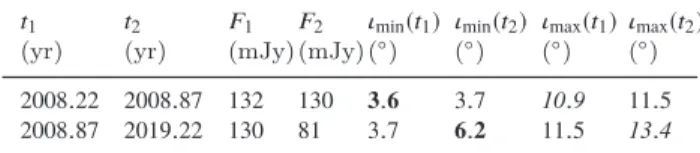
where the indices1,2mark the flux density and spin inclina- tion angle at two arbitrary epochs. We assumed a flat radio spectrum. In Fig.3, we marked three different epochs, t_A, t_B, and t_C, which are the starting epoch of the smoothed OVRO flux density curve, the epoch of the1.7- and5-GHz VLBA observations, and the last epoch of the smoothed OVRO flux density curve, respectively. The mean 15-GHz flux densities at these three epochs are F(t_A) = 132 mJy, F(t_B) =130 mJy, and F(t_C) =81 mJy, respectively, based on the (−4.67±0.13) mJy yr⁻¹ slope of the linear function fitted to the flux density data. Employing the minimum and maximum spin inclination angles allowed by the VLBI mea- surements at epocht_Bin the framework of the present binary model,ι_0,min=3.^◦7(withΓ=5,δ=9) andι_0,max=11.^◦5(with Γ=5,δ=5), and the flux density ratio in Eq.32, we calcu- late minimum and maximum spin inclination angles at the starting and finishing OVRO epochs. The resulting possible spin inclination angles are summarized in Table4. According to our results, the spin inclination angle could have changed by2.^◦5–2.^◦6over11yr in the framework of the present model.

By expanding the equation of motion in terms of the PN parameter, as we have seen, the dynamical evolution of the binary can be treated analytically while it pro- gresses through the inspiral phase where 0.001 . ε . 0.1 (Gergely & Biermann 2009; Levin et al. 2011). The time scale of the spin-flip is proportional toε^−9/2, while the time scale of the spin–orbit precession is proportional to ε^−5/2, when the spin is comparable to the orbital angular momen- tum (S₁ ≈ L). For Spikey, hε(t)i ≈0.001 means that if the flip occurs, it happens on a time scale more than10⁶ times longer than the time scale of the precession. We can safely state that if the slow decrease in the total flux density of Spikey is indeed due to the increase of the spin inclination angle, then the underlying mechanism should be the spin–

orbit precession, not the spin-flip.

4 DISCUSSION

4.1 No spike in the radio light curve

The long-term 15-GHz OVRO monitoring (Richards et al.

2011) covers the time of theKeplerspike (Smith et al. 2018) occured in 2011 June. Since the optical flare lasted only for about 15 days, it was poorly sampled in the radio. However,

Table 4.Possible jet inclination angles at the beginning (2008.22) and at the end (2019.22) of the OVRO flux density curve, based on the estimated minimum and maximum jet inclination values at the epoch of VLBI observations (2008.87). If we assume the minimum (maximum) inclination angle at 2008.87, the inclination angle changes from 3.^◦6 (10.^◦9) to 6.^◦2 (13.^◦4) in 11 years of the OVRO observations. These angles are marked by boldface (italic) in the table, respectively.

t1 t2 F1 F2 ιmin(t1) ιmin(t2) ιmax(t1) ιmax(t2) (yr) (yr) (mJy) (mJy) (^◦) (^◦) (^◦) (^◦) 2008.22 2008.87 132 130 3.6 3.7 10.9 11.5 2008.87 2019.22 130 81 3.7 6.2 11.5 13.4

there are 3 measurement points available in the OVRO data set for J1918+4937 in this time range, roughly at the be- ginning, middle, and end of the optical spike. From these data, there is no evidence for any radio brightening around Julian Date 2455724. On the contrary, the 15-GHz flux den- sity stays constant within the measurement errors.

Why is the radio emission unaffected in the SMBHB self-lensing scenario that Hu et al.(2020) proposed for the optical spike? There are two possible reasons. First of all, if only one of the BHs powers a radio jet, and this one is the lensing object in the foreground, then a radio magnifica- tion is obviously not expected. But even if the lensed object in the background is a radio-loud AGN, an optical spike is not necessarily expected to be coupled with a radio bright- ening. The optical emission of AGNs is known to originate mainly from the accretion disk on the scale of ∼ 10⁻⁵ pc (e.g. Koratkar & Blaes 1999). On the other hand, most of the 15-GHz radio emission comes from an ultracompact re- gion downstream the jet, on∼0.1−1pc projected scale (e.g.

Lobanov 1998). However, according to the model ofHu et al.

(2020), the SMBHB separation in the Spikey system is at least two orders of magnitude smaller. The entire binary system is therefore located well inside the region where the 15-GHz radio emission originates from. There is nothing to be gravitationally lensed in the Spikey system in radio, and even the superior angular resolution of VLBI is insufficient to directly resolve the companions.

4.2 Jet modeling with accurate binary parameters Modeling the observed high-resolution structure and kine- matics of VLBI jets in quasars is usually applied to infer parameters of suspected SMBH binaries (e.g.

Britzen et al. 2001;Lobanov & Roland 2005;Britzen et al.

2012;Valtonen & Wiik 2012;Caproni et al. 2013;Kun et al.

2014,2015,2018). In some of these cases, there is indepen- dent indication for the existence of the binary, e.g. from peri- odic optical variability. However, in the case of J1918+4937 (Spikey), the analysis of theKeplerlight curve byHu et al.

(2020) offers more than simply an indication. The measured optical spike is a unique phenomenon requiring special cir- cumstances, therefore its successful modeling with gravita- tional self-lensing and orbital Doppler boosting provides ac- curately determined BH masses, orbital parameters and ge- ometric constraints for the system (Hu et al. 2020). Unlike the usual practice, these parameters could therefore be fed directly into the VLBI jet model presented here (Sect. 3).

It was necessary to refine this model to allow for highly ec- centric binary orbits. In all earlier modeling, circular orbits were assumed for simplicity, as no reliable information about the binary orbital parameters were available.

We used VLBI imaging data taken at 1.7 and 5 GHz frequencies for Spikey, and also investigated the long-term OVRO flux density monitoring measurements at 15 GHz in the context of the SMBHB model proposed byHu et al.

(2020). The shape of the VLBI jet represented by the in- dividual component positions is remarkably consistent with the Spikey binary parameters. The constraints we obtained on Γ based on the single-epoch deep VLBI imaging of J1918+4937 at these two frequencies are not particularly strong (see Table3). Indeed, qualitatively, a jet with a given Doppler boosting factor can be produced either by relatively slowly-moving plasma blobs directed very close to the line of sight, or a fast jet with comparably larger inclination. Plau- sible values of Γ and the mean jet inclination angle with respect to the LOS (ι₀) could be provided only with multi- epoch VLBI jet kinematic studies (e.g.Lister et al. 2019).

However, utilizing also the available multi-epoch snap- shot VLBI imaging observations of J1918+4937 at the 8.4/8.7-GHz frequency band, we were able to estimate the apparent speed (β_app) in the jet from the measured linear proper motion of an inner jet component. The values of Γ andι₀ derived from βapp for the two possible values of the Doppler factor (δ=5and 9) fall within the parameter ranges set by our VLBI jet stucture model based on the parame- ters of the orbital motion of a SMBHB along eccentric orbit (Hu et al. 2020). Moreover, the values estimated from jet kinematics,Γ≈5−6andι₀ ≈6−12^◦, appear more consis- tent with the solutions in Table3, where the jet emitter is the smaller BH with massm₂.

As the optical emission likely arises from the gas bounded to the individual SMBHs in the binary sys- tem, the luminosity of the brighter minidisk (e.g.

Ryan & MacFadyen al. 2017) would be Doppler boosted and this minidisk is likely the one associated with the fastest- moving secondary SMBH (D’Orazio et al. 2016; Hu et al.

2020). The spike in the Kepler optical light curve of Spikey can be explained with the gravitational self-lensing if the larger-mass SMBH passes between the smaller-mass SMBH and the observer (Hu et al. 2020), magnifying the optical emission of the minidisk around the smaller SMBH. Also, Hu et al. (2020) successfully explained the long-term vari- ability in the light curve of Spikey by variable Doppler boost- ing due to the motion of the secondary SMBH. This means that at least the smaller SMBH has an accretion disk what we see in optical. Our VLBI jet model that utilizes the binary model ofHu et al.(2020) is indeed more consistent with the jet parameters derived from VLBI monitoring of Spikey if we assume the secondary SMBH is the jetted one in the system. Notably, the χ² values also indicate slightly better fits for those solutions, and if the secondary-mass SMBH is the jetted one, the parameterκ_i is much better constrained, without reaching the limiting value0^◦.

As it is often seen in radio-loud AGNs, the OVRO mon- itoring light curve of Spikey (Fig.3) is rather complex. Vari- ations with characteristic time scales of∼1yr and shorter are superimposed on a generally decreasing trend in flux density. We attempted to relate this long-term trend seen during the entire monitoring period of more than11 yr to