insulators
BMEVIVEM173
Koller, László
Novák, Balázs
Tamus, Ádám
Electrical switching devices and insulators
írta Koller, László, Novák, Balázs, és Tamus, Ádám Publication date 2012
Szerzői jog © 2011
2. Switching transients ... 6
1. Switch-on processes ... 7
1.1. Fault far from the generator ... 7
1.2. Switch-on of a transformer under no-load condition ... 10
2. The electric arc ... 12
2.1. V-I characteristics of the steady-state arc ... 13
2.2. Dynamic arc characteristics ... 14
2.2.1. Arc characteristics in HV circuits ... 14
2.2.2. Arc characteristics in LV circuits ... 15
2.2.3. Arc quenching and re-ignition in a switching device ... 15
3. Switch-off processes ... 18
3.1. Ideal interruption of an HV terminal fault ... 18
3.2. Interruption of small inductive currents in HV circuits ... 21
3.3. Interrupting a LV terminal fault ... 23
3.3.1. Interruption without current limitation ... 23
3.3.2. Interruption with current limitation ... 24
3. Thermal transients ... 26
1. Slow temperature rise ... 28
2. Fast (short-circuit) temperature rise ... 29
3. Permitted temperature rise ... 30
4. Mechanical transients ... 32
1. Force calculation based on Biot-Sawart law ... 33
2. Force calculation based on the change of magnetic energy ... 34
3. Direction of force ... 35
4. Repulsive force in current constrictions ... 36
5. Effect of electrical transients ... 36
5. General rules of switching device selection ... 38
6. Structure and operation of electrical switching devices ... 39
1. Relays and releases ... 39
1.1. Properties, classification ... 40
1.2. Electromagnetic relays and releases ... 41
1.3. Magneto-mechanical relays ... 43
1.4. Thermo-mechanical relays ... 43
1.4.1. Bimetallic switch ... 43
1.4.2. Thermistor relay ... 44
2. Circuit breakers ... 44
2.1. High voltage circuit breakers ... 45
2.2. Low voltage circuit breaker ... 48
2.2.1. Structural elements ... 49
2.2.2. General purpose circuit breakers ... 50
2.2.3. Current limiting circuit breakers ... 53
2.2.4. Miniature circuit breakers (MCB) ... 55
2.2.5. Selection ... 57
3. Fuses ... 60
3.1. Medium voltage fuses ... 61
3.1.1. Short-circuit operation ... 61
3.1.2. Overload operation ... 65
3.1.3. Structure ... 67
3.2. Low voltage fuses ... 68
3.2.1. Structure and properties ... 68
3.2.2. Operation during short-circuit ... 70
3.2.3. Operation during overloads ... 73
3.2.4. Selection ... 77
4. Disconnectors ... 78
Electrical switching devices and insulators
5. Load break switches ... 81
5.1. Mechanical switches ... 83
5.1.1. Biased switches ... 84
5.1.2. Rotary switches ... 85
5.1.3. Snap action switches ... 87
5.1.4. Contactors ... 90
5.2. Semiconductor switches ... 101
6. Switching device combinations ... 103
6.1. Medium voltage switching device combinations ... 103
6.2. Low voltage device combinations ... 104
7. Overvoltage protective devices ... 107
7.1. High and medium voltage overvoltage protecting devices ... 107
7.1.1. Rod gap lightning arrester ... 108
7.1.2. Metal-oxide surge arresters ... 108
7.2. LV overvoltage protecting devices ... 109
7.2.1. Metal oxide surge arrester (varistor) ... 109
7.2.2. Gas discharge tube (GDT) ... 110
7.2.3. Transient voltage suppression diode (TVS) ... 111
7. Properties and design of insulations ... 112
1. Operational stresses of insulations ... 112
2. Fundamentals of insulation design ... 112
8. Diagnostics of insulations ... 114
1. Fundamentals of examination of insulations ... 114
2. Methods of insulation diagnostic tests ... 115
9. Examples ... 117
1. Example ... 117
2. Example ... 117
3. Example ... 117
4. Example ... 117
5. Example ... 117
6. Example ... 117
7. Example ... 118
8. Example ... 118
9. Example ... 118
10. Example ... 118
11. Example ... 118
12. Example ... 119
13. Example ... 119
14. Example ... 119
15. Example ... 119
16. Example ... 119
17. Example ... 119
18. Example ... 120
19. Example ... 120
20. Example ... 120
21. Example ... 120
22. Example ... 120
23. Example ... 120
24. Example ... 120
25. Example ... 121
26. Example ... 121
Bibliography ... 123
courses. According to its title, the book presents two, highly related technical fields. Five chapters deal with electrical switching devices and three with insulation technology. The first, introductory chapter defines some essential concepts necessary for understanding the remaining of the book.
Electrical devices do not generate, distribute or measure electric power. Among the electric power consuming equipment, we do not consider the motors, and lighting units as electrical devices. However, the range of electrical devices is still very wide, and we deal only with electrical switching devices.
The students of MSc subjects must have a basic knowledge of the field from their previous BSc studies.
Considering that there is no sharp boundary between the bachelor and master courses, this book discusses those parts of the BSc subject, which are highly relevant for conceiving the new material.
The different courses, subjects, and topics have continuously changed and developed during the years of their existence. This entailed the publication of several different lecture notes related to each other. The contents of the current book are based on the lecture notes published in [1–3]. Although these three books cover a wide range of related topics about electrical switching devices and equipment, their structure does not provide an easy overview of the field. We tried to fulfill the need for a clear overview by restructuring and rewriting the existing material. We complemented the previous text with new chapters, and added new summaries and explanations.
However, because of size limits, we had to omit some special or less up-to-date topics. To make comprehension easier, we redrew most of the figures in colors, and in one case, we attached an animated drawing.
We hope that the students will be able to use our electronic lecture notes effectively during their studies.
Budapest, September 2011.
only do they make the transmission of electric power possible, but their failure can lead to losses – due to the interruption of power distribution, or the damage of valuable equipment – much-much higher than their own value. Therefore, electrical switching devices must be reliable, and owing to their high number in electric power systems, their manufacturing must be cost effective. To achieve efficient transmission of electric power, different voltage levels are utilized in power systems. Higher the transmitted power or longer the distance of transmission, higher is the rated voltage of the system (V r=0.4; 10; 20; 35; 120; 220; 400; 750 kV). Obviously, the rated voltage of the electrical switching devices has to exceed that of the network, in which they are installed. Consequently the rated voltages of high voltage equipment are 12, 24, 40,5, 145, 245. 420 and 787 kV respectively. Similar to the electrical grid, the switching devices can be classified as “low”, “medium”, “high”,
“very high” and “ultra high” voltage types (Fig. 1.1). However, the more simple classification of low voltage (LV; <0.4 kV), medium voltage (MV; 12, 24, 40.5 kV) and high voltage (HV; 145, 245. 420 and 787 kV) is more general.
Electrical switching devices are rarely standalone units, usually several of them are installed together at specific points of the electrical systems, forming – together with connecting elements – switchgears. Switchgear is a general term covering switching devices and their combination with associated control, measuring, protective and regulating equipment, also assemblies of such devices and equipment with associated interconnections, accessories, enclosures and supporting structures.
Fig. 1.1. Rated voltages of electrical switching devices
Besides their rated voltage, electrical switching devices must be appropriately selected according to their purpose and function. In accordance with this function, first we have to discuss the normal operating, rated, overload, and fault (short-circuit) currents occurring in normal and faulty states of the electrical systems. These system states can be made or terminated by electrical switching devices, but they can be caused unintentionally by faults (short-circuit or disruption) as well.
Turning on or off consumer loads corresponds to the normal operation of three-phase systems. Although sometimes, the elements of electric power systems have to make switching operations during no-load conditions too (e.g. turning on/off a transformer or transmission line which is not in use).
Switching operations can occur in a faulty state of the system as well, like during overloads or short-circuits. For instance, turning on a faulty equipment can result in making a short-circuit current. The electrical switching devices are responsible for the automatic disconnection (interruption) of this excessive current.
We discuss the characteristic currents of the different system states by means of simplified single-phase models of the symmetrical three-phase systems.
Introduction
Fig. 1.2. Normal condition
/Figure 1.2 shows the one-line equivalent circuit of the electric power system during normal conditions. The reactance and impedance of an inductive operating load having inductance L and resistance R per phase:
(1-1)
where, in case of frequency f, the angular frequency:
Modeling the network between the switching device K and the generator having V p phase voltage by an inductance L m and a resistance R m, the reactance and impedance of the connecting network:
(1-2)
To achieve economic power supply, the rate between the elements of the connection link and the load should be kept such, to make the load impedance and the resultant impedance Z r of the network almost equal:
(1-3)
and as a consequence:
(1-4)
Consequently, the operati ng current I o flowing through the load and the serial elements of the connection:
(1-5)
The operating current must not exceed the rated current I r, since the serial elements of the network cannot withstand a higher current without detrimental overheating. The smallest load impedance corresponding to I r:
(1-6)
Fig. 1.3. Overload condition
In Fig. 1.3, the equivalent circuit representing a fault (overload) condition of the system can be derived from the previous case of normal operation by inserting a load impedance Z parallel to the rated load impedance Z r. Since in this case
operation of devices producing them.
In Fig. 1.4 a fault (short-circuit) condition occurred during normal operation in the electrical system. The impedance Z of the load is shunted by a short-circuit impedance of zero value in the equivalent circuit.
Fig. 1.4. Fault (short-circuit) condition
Considering relation (1-4), the short-circuit current I sc is much higher than the rated current, since I sc is limited only by the impedance Z m of the network:
The huge short circuit current would damage the electrical equipment in a very short time, therefore it must be interrupted instantly or (possibly without a delay) as fast as possible.
After describing the rated voltages and the different states and current levels of the electrical systems, we introduce the reader to the different types of electrical switching devices used in electric power transmission and distribution. The switch K in the previous figures (1.2 … 1.4) can be substituted by these switching devices having different functions and purposes. We provide detailed descriptions later in chapter 6, which discusses the construction and operation of electrical switching devices.
1. The high, medium, and low voltage circuit breakers (CB) are mechanical switching devices that can make or break currents during normal or fault (including short-circuit) conditions. Mechanical means that switching operation is accomplished by separable opening or closing contacts. Furthermore, if their contacts are closed, CBs have to be able to conduct operating currents for an unlimited and fault currents for a limited time.
2. The low and medium voltage fuses are electrical switching devices that automatically interrupt excessive currents lasting for a specific time by melting one or more metal wires or strips connected parallel (fuse element) inside a fuse link and quenching the electric arc, which occurs after melting. The fuse element has a relatively small cross sectional area, thus it can be considered as an intentionally weakened point of the electrical network. The fuse has two functions: first of all it provides protection against short circuits and limited protection against overload currents. It has to be able to conduct rated or less than rated currents for an unlimited time. Consequently, the function of the fuse is similar to that of the CB, but providing interruption only once. It is a protective device in the electric power system.
3. The high and medium voltage disconnectors or isolators are mechanical switching devices, which provide complete insulation distance called isolation distance between their open contacts. They have to satisfy safety and electrical requirements regarding their open contacts that is, as their major task, they have to provide safe and visible separation between parts of the electrical system. They have negligible current interrupting capability and are only used in the off-load condition. They can be operated only if negligible current flows through them, or if the voltage across their contacts is insignificant. If their contacts are closed, they have to be able to conduct rated current for unlimited time and they have to withstand the thermal and dynamic effects of short-circuit currents. Their secondary task is to arrange the path of the current. An example is a double busbar system, where disconnectors provide the way for the power flow between the busbars.
Disconnectors are often equipped with earthing switches or earthing knives.
4. The medium and low voltage (mechanical or semiconductor) load break switches can make or break currents during normal, operating conditions. These include some specific overload conditions as well.
Furthermore, they have to be able to conduct currents different from normal conditions (faults) until the
Introduction
protective measures are taken. The mechanical contactor is a special load break switch. An electromagnet provides the driving force to close its contacts; therefore it has a special construction and tasks. The semiconductor switches form a separate group of load break switches. By controlling the conductivity of semiconductor elements in them, they can turn on or off electrical circuits. They can be used also for similar tasks as the contactors.
5. Owing to their smaller size, easier installation and favorable price, medium and low voltage combinations of switching devices providing the tasks of two or three basic units are used mostly in indoor applications.
They can be classified in two groups:
The manufacturer assembles serial connected switching devices in a single unit. This does not really result in new device types, only the on-site installation work becomes simpler. The basic switching devices can be easily recognized in these units (e.g. disconnector-fuse, switch-fuse, switch-disconnector-fuse, integrally fused circuit- breaker).
New constructions made from basic switching devices (e.g. fuse-switch, fuse-disconnector, fuse-switch- disconnector).
1. High and low voltage overvoltage protecti ng devices (spark gap, surge arrester, varistor, etc.) play a crucial role in electric power systems, although they are not serial elements. Their task is to limit the level of overvoltages in an electrical network. During most of their operating time they remain idle, they do not contribute to the operation of the system. They cannot be activated directly or intentionally, although overvoltages in the system or in the equipment automatically trigger their operation.
2. Automatic protection relays and releases provide safety and improve the reliability of the transmission, distribution and consumer electrical systems. The protection relays and releases can be standalone units, or replaceable or fixed elements of other switching devices (e.g. CB), or they can provide auxiliary protective functions (e.g. with contactors). Their task is to continuously monitor different parameters of electrical systems or equipment. Based on the variation of these parameters they detect faults or other abnormal conditions, enable fault clearance, terminate abnormal conditions, and initiate signals or indications automatically without human interaction.
Fig. 1.5. MV/LV transformer substation
Substations and transformer stations are situated at the connection points of power transmission or distribution lines in the power system. The incoming and outgoing lines are connected to busbars by means of electrical switching devices. As an example, Fig. 1.5 depicts the simplified one-line diagram of one fraction of an industrial MV/LV transformer substation. An underground cable supplies power to the single busbar substation through a disconnector with an earthing knife (DE). The fault protection of the cable is accomplished by a circuit breaker in the substation at the supply side of the cable. One of the MV motor circuits is protected and switched by a withdrawable circuit breaker (CB), whereas the other by a withdrawable switch-fuse. Besides the CB protected motor circuit connection, the MV switchgear includes the connection for the MV/LV transformer
2. fejezet - Switching transients
Switch on and off operations induce energy change in an electric power system, therefore electric transients – and between the separated contacts of mechanical switching devices, the effects of electric arc – have to be taken into account until the network reaches quasi steady-state. The transients and the arc can temporarily have adverse effects, as they increase the electrical, mechanical and thermal stresses of the power system. Since switching devices are part of the system, their operation is also influenced by these effects.
In the circuit representing a fault condition in Fig. 1.4, let the switch K model the contacts of a real switching device (e.g. CB). Figure 2.1 illustrates the steps of its operation during making and breaking a fault current.
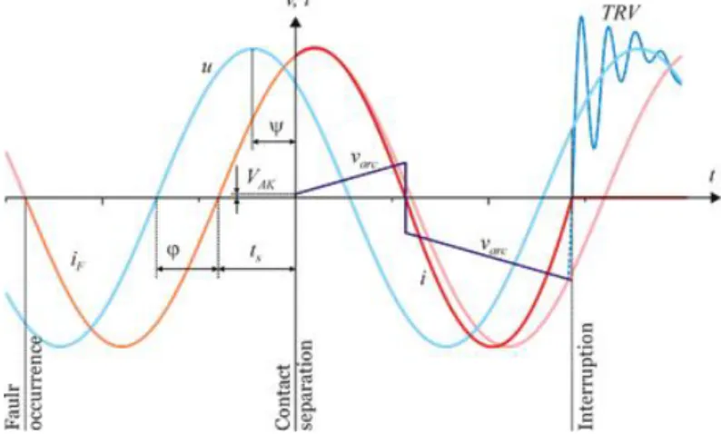
While the contacts are open (1), no current is flowing in the circuit (i=0). During a closing operation, before the contact members reach each other, a sparkover occurs initiating an electric arc. A fault current of i=i arcin flows through the arc (2). However, this arc can occur only on high voltages and its duration is very short, since it extinguishes after the contacts get closed. At this moment, a prospective short circuit current i=i SC starts to flow through the contact members (3). This short circuit current would be harmful for the system; therefore a protective relay automatically triggers the CB to interrupt it. After the protection trips the CB, the contact members start to separate and – both on LV and HV – an electric arc starts burning between them (4). The constriction of the current to small spots on the contact surfaces explains the fact that there is always an arc between the opening contact members during current interruption. During opening, the number and the area of the contacting spots rapidly decreases, making the current density so high at some points that its heat melts and vaporize the surface. The ionized metal vapor provides a conducting path for the arc. If the arc was a perfect conductor, in a circuit with sinusoidal supply voltage, the prospective short circuit current i SC would continuously flow at least until its first current zero. In reality however, the electric arc is a non-linear, resistive element of the circuit, and the dynamic arc of an AC circuit makes the current i=i arc distorted that is non- sinusoidal. This current lasts at least until its first current zero. The interruption is successful, if the arc finally extinguishes, or more precisely, if re-ignition of the arc can be inhibited at or close to the current zero. If re- ignition happens, i arc further flows up to its next current zero. The moment of the current zero and also the highest value of the arc current are both influenced by the shape and magnitude of the arc voltage. In HV circuits, the voltage of the relatively low resistance arc is negligible compared to the supply voltage: the arc modifies the current time function only close to current zero. The situation is different in LV circuits, where the arc has relatively high resistance, and its voltage is comparable to – sometimes its momentary value is even higher than that of – the supply voltage. In this case, the arc current significantly differs from the arc-free prospective current. Both the peak and the moments of current zeros of the arc current and the prospective current can be different. This difference is the most pronounced with current limiting circuit breakers. The contact members of these devices are separating so fast and the arc voltage is increasing above the momentary value of the supply voltage so rapidly that the peak of the arc current (let-through current) becomes significantly less than the peak of the prospective current. Fuses limit the current similarly, although in their case the melting of the fuse element corresponds to the contact separation of circuit breakers. The fault current in DC circuits can be interrupted that is, current zero can occur only, if the arc voltage between the contacts exceeds the DC supply voltage. Even current limitation is possible in this case, if the contacts separate before reaching the steady-state fault current.
The interruption is successful (5), if the arc finally quenches, namely it cannot re-ignite. This results in the initial state (1) of the switching device in Fig. 2.1. A transient recovery voltage (TRV) appearing between the contact members after a current zero can cause dielectric or thermal re-ignition of the arc. The time function of the TRV is determined by the elements of the circuit (resistances, inductances, capacitances) and the resistance of the electric arc.
Fig. 2.1. Operating states of the contacts of an electric switching device
We use the electrical switching devices mostly in three-phase AC power transmission and distribution systems.
Therefore, by operating them, we modify the operating state of these systems (even if we just turn on a lamp in a room with a single-pole switch). Furthermore, the switching operations are often asymmetric, the network parameters are distributed and the elements of the network are non-linear (e.g. the electric arc). Precise modeling of such complex processes would be very complicated, therefore we use simplified models to explain and demonstrate the nature of switching processes. Unfortunately, the simplest non-linear, single-phase,
Furthermore, at low voltages, even the current type is an important influencing factor. The voltage level determines the values and rates of network parameters (e.g. power factor) as well. Consequently, it is essential to classify also the electric transients according to voltage and – at low voltages – according to current type.
There are situations, where these classifications are not relevant, since the given physical process can happen both at low and high voltages. We note here that, because of the limited size of this book, we discuss only AC phenomena more typical in practice. We will follow the operating states shown in Fig. 2.1 during our discussion. First we treat the switch-on transients, second the properties of the electric arc between the contacts, and finally the processes taking place during switch-off operations. We discuss the electric transients caused by fuses together with the structure and operation of the electric switching devices in another chapter.
1. Switch-on processes
In AC circuits, the supply voltage affects the switch-on processes only through the parameters of the circuit elements; therefore we do not distinguish switch-on processes regarding the voltage level.
In Fig. 1.2, we have seen that the equivalent circuit must include a resistance and an inductance representing the three-phase synchronous generator. Due to the increase of current during a short circuit, the values of the generator parameters – especially the inductance – significantly change. In most of the practical cases, we neglect this change, since constant inductances and other constant elements – representing the transformers, transmission lines, etc. – with much higher values than that of the generator’s are connected in series with the generator. We can say that a circuit with constant parameters represents a fault far from the generator. We discuss this fault type and the electric transients caused by switching on of a load-free transformer in the followings.
1.1. Fault far from the generator
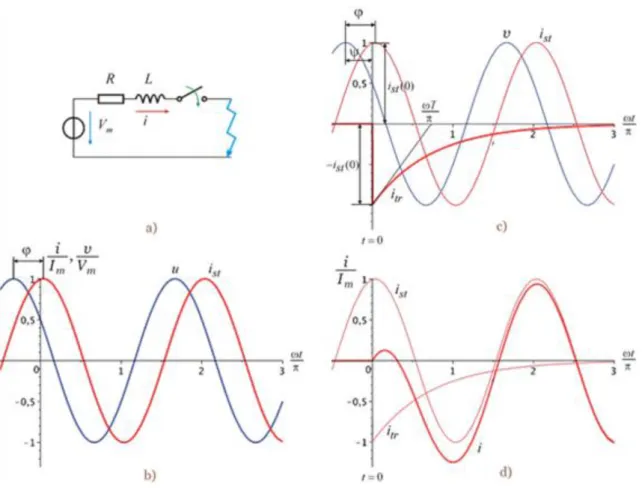
Figure 2.2.a shows the equivalent circuit modeling a fault current switch-on. The lumped resistance and inductance R and L represent the generator, lines, transformer, etc. together. Furthermore, v = V m⋅ cos ω t is the momentary value of the supply voltage. The switching device is in open position, current has not been flowing in the circuit, and thus the inductance is energy-free. The fault occurs and a current starts to flow, when the switch is turned on at the moment of t=0. The time function i(t) of this current depends not only on the phase angle υ, but also on the moment of fault occurrence.
The fault current reaches steady-state after a long time, the maximum of its momentary value:
(2-1) where
The steady-state current lags behind the supply voltage by an angle of
therefore its time function:
(2-2)
Switching transients
Figure 2.2.b shows this time function together with the supply voltage, with ω t/ π on the horizontal axis of the diagram. The fault can randomly occur in any moment. If the fault occurs exactly at the moment of a steady- state current zero, then the steady-state current will start to flow immediately. In this case, the time-function of the fault current coincides with that of the steady-state current: i(t)=ist(t). The zero steady-state current at the moment of switch-on ensures that the inductance is energy-free in this favorable case. In any other case, the steady-state current differs from zero at the moment of switch-on. Since the inductance must be energy-free, a transient current component i tr compensating this finite current appears in the system. Therefore the time- function of the fault current in a general case:
(2-3)
The moment of switch-on, t=0 determining i st(0) is indicated by the vertical axis for a general case. This moment is shifted by a ψ switch-on angle in the positive direction from the positive crest of v. Since no current has been flowing before t=0, and because the current cannot jump in a circuit including an inductance, current cannot flow either at the moment of t=0. Therefore
from which the initial value of the transient component:
The initial magnitude of the transient current equals to that of the steady-state current, but with opposite sign.
The transient current exponentially decreases from this initial value and tends to zero after a long time. The ohmic resistance of the circuit results in the damping in the system. The transient component is plotted in Fig.
2.2.c, considering that
(2-4) where
(2-5)
is the time constant of the circuit.
Fig. 2.2. Fault far from the generator: equivalent circuit (a), time functions (b-d)
The sum of i st(t) and i tr(t) results in the time-function of the fault current i(t) that we wanted to determine:
(2-6)
This current, together with its two components, is plotted in Fig. 2.2.d. It can be clearly seen that its peak is higher than I m.
Fig. 2.3. Case of the possible highest current peak
The initial value of the transient current i tr(0) and consequently the peak of the resultant current depends on the moment of current initiation. In a circuit with phase angle υ , this moment is determined by the switch-on angle ψ. The most unfortunate time instant of current initiation generates the possible highest peak (I* m). In any inductive circuit, this time instant belongs to ψ=±π/2 that is, when the current starts exactly at the moment of supply voltage zero (see Fig. 2.3). In a solely inductive circuit (φ=π/2), the peak factor
Switching transients
(2-7)
is k p=2. Nevertheless, there is always a resistive component in a real circuit, therefore, when calculating the effects of the current, an average value of k p=1.8 is acceptable.
Figure 2.4 shows the “favorable” situation mentioned before (ψ-υ=π/2), when transient does not take place, leading to a peak factor of k p =1. Figure 2.5. depicts another special example, when the transient starts from its possible highest value, namely when the current was initiated at the steady-state current peak (ψ-υ=0). In this case, the possible maximum of the resultant current is less than – in solely inductive circuits equal to –I*m
corresponding to a switch-on at voltage zero.
Fig. 2.4. No transient component
Fig. 2.5. Possible highest transient
1.2. Switch-on of a transformer under no-load condition
Although the steady-state no-load current of a transformer is much less than its rated current, switching on a load free transformer can cause a transient that can reach even 100 times the steady-state for a short time. This in-rush current is so high that it can amount to several times of the rated current.
Fig. 2.6. Equivalent circuit
To understand this adverse phenomenon, let us consider the circuit of Fig. 2.6, where Ψ(i) represents the magnetic flux of the transformer, as a non-linear function of its current. Applying Kirchoff’s II. law to the circuit:
(2-8)
where ψ is the switch-on angle.
To solve the differential equation, we have to know the non-linear relation ψ(i) that is, the magnetization curve B-H of the transformer. The hysteresis of the magnetization curve makes the problem even more complicated.
The sinusoidal steady-state flux Ψ st (i) lags behind the sinusoidal supply voltage by an angle of π/2. If we know the hysteresis curve Ψ (i) st valid in steady-state, from the flux we can plot the distorted steady-state current point by point. This current is the no-load current of the transformer (Fig. 2.7).
Fig. 2.7. Obtaining the load-free steady-state current
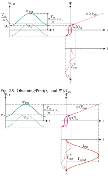
To begin with, we assume that the transformer’s yoke did not have any remanent flux at the moment of switch- on (Ψ(0)=0), but the switch-on occurred at the worst time instant, namely at voltage zero. This time instant corresponds to the angle of ψ=-π/2. Figure 2.8 depicts the resultant flux Ψ (t) in this case. In reality however, there is always a remanent flux in the yoke of a previously used transformer. This remanent flux can be positive or negative. In our case, the positive value results in higher initial flux and therefore in higher surge current. By adding Ψ r to Ψ (t), we can obtain the flux Ψ init (t) valid at the beginning of the switching process.
Fig. 2.8. Obtaining Ψ (t), if Ψ r =0
To obtain the time function i(t)init of the initial current, we have to know the initial flux curves Ψ (i) init originating at the corners of the hysteresis loops as well. Like in Fig. 2.9, the first section of these curves can be approximated by a straight line starting from the point of the positive remanent flux (Ψ r). Together with the initial flux Ψ init (t), this low steepness line yields the time function of the initial current i init (t), as it can be seen in Fig. 2.10. In short, the causes of the initial large current surges are the following: switch-on at voltage zero, the remanent flux, and the low steepness of the magnetization curve.
Switching transients
Fig. 2.9. ObtainingΨinit(t) and Ψ (i) init
Fig. 2.10. Obtaining i init (t)
Table 2.1 demonstrates for different – core- and shell-types of – transformers that, depending on the rated power (S) of the transformer, the maximum of the no-load initial current surge (I minit) can significantly exceed the peak of the rated current (I mr). The ratio I minit /I mr is higher with core-type – where the flux lines are connected with each other – than with shell-type of transformers.
Table 2.1.
I minit /I mr
S [MVA] core-type shell-type
2 3 2
. . .
. . .
. . .
20 8 5
2. The electric arc
Fig. 2.11. Voltage distribution along the arc length
The electric arc consists of ionized gas, and it originates and ends on small spots on the electrodes. The spot moves in a rapid and irregular way on the cathode. The spatial stability of this movement depends on the cathode material. Materials with high melting temperatures (e.g. wolfram) ensure high cathode temperatures, resulting in a relatively stable arc. The electric potential distribution along the arc is plotted against the arc length in Fig. 2.11. In the vicinity of the anode and the cathode, charge carriers with opposite sign to that of the electrodes are generated. There are three distinct regions of an electric arc, namely the cathode drop region, the arc column or arc plasma region and the anode drop region. The cathode is negative, the anode is positive and the arc column – situated in between anode and cathode drop regions – is electrically neutral, as it contains equal number of ions and electrons. The length of the anode and cathode drop regions (l a and l c) is small; it is of the order of micrometers, and l a l c. It can be seen that the electric field strength is much higher in these regions than in the arc column. If the arc length is short, the voltage along the arc column becomes negligible, the arc voltage is determined by the anode and cathode drops (in an extreme case, with zero arc length, only the latter two contribute to the arc voltage). Arcs burning between the mechanical contacts or between the deion plates of LV switching devices can be considered „short”. Therefore, the physical processes close to the anode and the cathode explain the behavior of such arcs in LV circuits. The properties of “long” arcs between the mechanical contacts of HV switching devices are mostly determined by the physical processes in the arc column.
This chapter summarizes only those properties of the switch arc, which help us to understand how the arc influences the switching processes in electrical circuits.
We say that the arc is steady-state, if the momentary value of the current flowing through it is constant. If this condition is not satisfied, the arc is dynamic, or, in the case of periodically varying current, the arc is quasi steady-state. It is worthy of notice that the arc is always dynamic in a switching device, since the current continuously changes during the switch-off process. The steady-state arc is a non-linear circuit element, its resistance is not a constant value; a characteristic curve represents the relation between its current and voltage.
First we will introduce the steady-state arc characteristics, and based on it, we continue with the characteristics of the dynamic arc, discuss its properties in LV and HV circuits and its behavior during quenching and re- ignition.
2.1. V-I characteristics of the steady-state arc
The diagrams in Fig. 2.12 show arc characteristics at constant pressure (p=const.) with different arc lengths (l 2
l 1). It can be clearly seen that until about 1000 A the steepness of the curves is negative, indicating that larger current results in lower arc voltage. After a roughly horizontal section, further increase of the current above 10000 A goes together with rising arc voltage. This effect may be explained by the electrodynamic forces, which reduce the cross section of the arc channel (current filaments of the same direction attract each other).
Switching transients
Fig. 2.12. Steady-state arc characteristics at constant pressure
2.2. Dynamic arc characteristics
If a time varying current (di/dt≠0) flows through the arc, it can be modeled by dynamic characteristics. By starting from a single point of the steady-state V-I curve, and increasing the current at a finite rate di/dt i
1 to i 2, the voltage of the arc falls above the steady-state diagram. After getting to i 2 the arc voltage needs some time to reach its steady-state value corresponding to i 2 (Fig. 2.13). The phenomenon may be explained by the thermal inertia of the arc. In other words, the temperature and conductivity of the arc cannot follow the change of its current instantly; it tries to keep its conductivity belonging to i 1. Similarly, if we reduce the current from i
2 to i 1 by the rate of di/dt -state characteristic curve. Theoretically, during an abrupt current jump (di/dt=∞) the conductivity could not follow the change of the current at all, the arc would become a linear element, Ohm’s law would be valid, and the resistance of the arc R arc would become constant. The transient behavior and the thermal inertia of the arc can be represented by a thermal time constant τ arc. Its value is in the order of10-6...10-3 s, the lower limit typical in HV circuit breakers, whereas the higher one in air at atmospheric pressure.
Fig. 2.13. Dynamic arc characteristics
During switching processes, the current is not constant, therefore the arcs are dynamic. In the following section we discuss the different arc characteristics in HV and LV circuits, and we deal with the quenching and re- ignition of the electric arc.
2.2.1. Arc characteristics in HV circuits
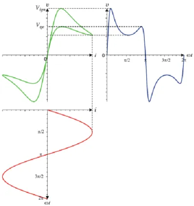
With AC supply voltage, the current flowing through the arc is time varying, and quasi steady-state characteristics are valid. These characteristics depend on the values of the circuit elements as well. During switching off an HV circuit, the arc can be considered quasi steady-state, since the current can last up to several half cycles, and as the supply voltage is much higher than the arc voltage, the current hardly differs from sinusoidal. The diagrams in Fig. 2.14 show quasi steady-state arc current and voltage time-functions, together with the characteristic curve representing the relation between them. These diagrams are based on measurements and theoretical deductions valid for relatively long arcs. The corresponding current and voltage values follow a hysteresis loop. The polarities of the arc current and voltage are the same at every moment, and their zeros occur always at the same time. This means that the AC arc extinguishes before and re-ignites after every current zero.
Peaks (V ign and V qe), typical for extinction and re-ignition, can be easily recognized in the voltage time- functions at these time instants.
Fig. 2.14. Arc voltage and current in an HV circuit (arc hysteresis and time functions)
2.2.2. Arc characteristics in LV circuits
The voltage of a short arc in an LV circuit is comparable to, or sometimes is even higher than the supply voltage. Consequently, the time-function of the prospective current significantly changes after initiation of the arc. For instance the non-linear arc results in a distorted current in an AC circuit. The anode and cathode drops form a major part of the arc voltage, what is even more pronounced, when several short (0.3…1.0 mm) arcs are connected in series, each contributing to the voltage with its own anode and cathode drops. Therefore, the well- tried theories of long HV arcs are not valid in LV circuits. The time-function v arc(t) of the arc voltage in an LV switching device majorly differs from the quasi steady-state shape of Fig. 2.14 appearing in an HV unit. For instance, it does not have any well recognizable extinction and re-ignition peaks. The arc extinguishing mechanism of a switching device and the separation speed of the contacts determines this time function, and – according to measurements – its mathematical representation is rather simple:
(2-9)
where t is the time passed since the initiation of the arc (in case of mechanical contacts, the time from contact separation). Knowledge of this voltage and the parameters of the DC or AC low voltage circuit, makes possible to calculate the current i(t) flowing through the arc.
2.2.3. Arc quenching and re-ignition in a switching device
The arc disappears if its current becomes zero. In case of DC interruption, the switching device itself must provide this condition by modifying the arc properties. With AC supply, the arc disappears at a natural current zero in HV circuits, or at a current zero determined by the arc voltage in an LV circuit. Another possibility is that the arc becomes unstable, and disappears shortly before these current zeros, resulting in a sudden drop of the current. This is the case of current chopping. If the switching device is capable of preventing the re-ignition, the arc eventually quenches, the interruption is successful. If re-ignition cannot be inhibited, the arc appears again and –in case of AC circuits – remains until the next current zero.
After current zero, an ionized channel called post-arc remains at the place of the arc. Only de-ionizing processes take place in this channel and the arc eventually quenches, if current does not flow for a prolonged period, and if
Switching transients
there is no electric field strength between the electrodes. Re-ignition can occur, if ionization surpasses de- ionization.
a) The arc can re-ignite in a gas if:
1. the recovery voltage (TRV) between the contacts generates a post-current or remanent current through the post-arc, and this current affects the thermal equilibrium of the post-arc such, that the heat content (and temperature) of the arc increases: dQ/dt>0 (thermal re-ignition),
2. or the thermal processes are negligible (interrupting low currents at high voltage; or at low voltage, where the electrodes cool the arc), and fast increasing TRV results in collision ionization, which generates a re-strike (spark breakdown or dielectric re-ignition).
Fig. 2.15. Time-function of re-strike voltage of a LV arc burning in air
At low voltages, the electrodes have a relatively high mass, which results in powerful cooling and de-ionization of the arc burning in air. Therefore in LV equipment, the typical re-ignition is spark breakdown. To decide if the interruption can be successful, we have to know the time variation of the returning dielectric strength or breakdown voltage (v ign) of the gas between the electrodes. A typical example of this re-strike voltage is illustrated in Fig. 2.15. The voltage v ign reaches a V ign0 value in a very short time (1...3 μs) as the space charge in front of the cathode is neutralized rapidly. Higher the arc current, lower this V ign0, since stronger current generates more charge carriers before it reaches its zero. The value of V ign0 can be in the order of 160…210 V, when interrupting low currents (I<100 A). This voltage is commensurable with the supply voltage. Although if the current exceeds 1000 A, it is much less, V ign0≈10 V. The second, low gradient (k) region of the re-strike voltage corresponds to the neutralization of the arc column. The formula
(2-10)
provides a good approximation of the re-strike voltage time-function. As a consequence, the arc extinguishing methods in LV equipment are mostly based on increasing V ign0. This can be accomplished by multiplying the number of electrode gaps (more contact pairs in series) or by splitting the arc into small pieces (deion plates).
At high voltages, depending on the current to be interrupted, both thermal and dielectric re-strikes can occur.
Fig. 2.16 shows the time-function of the re-strike voltage v ign valid for both mechanisms. During calculations, we have to take into account the lower voltage values. For instance, with the current of I 1, the thick line provides the time-variation of the re-strike voltage. The curve corresponding to dielectric re-ignition can be approximated by formula (2-10) in this case as well.
must also be considered. The HV switching devices have to accomplish two tasks to inhibit arc re-ignition. One of them is to reduce the arc energy
(2-11)
before the current zero, namely before the arc annihilates. The other one is to promote de-ionization processes in the post-arc. Sometimes these aims conflict each other; for instance, cooling helps the de-ionization, but at the same time it increases the arc energy.
The general methods of arc quenching (preventing of re-strike) in gases at high voltage can be summarized as follows:
- raising the pressure (breakdown strength increases, number of ions is reduced), - applying quenching material and cooling (helps de-ionization processes), - removing ions by forced flow of the gas,
- lengthening the arc, increasing the electrode distance (breakdown strength increases).
Fig. 2.17. Equivalent circuit of a CB terminal fault
Smaller arc time constant τ arc impedes both the thermal and the dielectric re-strikes more effectively. However, over-reducing τ arc – e.g. by powerful cooling, namely by increasing the heat power transmitted from the arc – can make the arc unsteady close to the current zero, resulting in current chopping. Therefore it is important to discuss the stability of the arc. Mayr was the first, who investigated the stability of the arcs burning in gases. He examined the behavior of the arc in the circuit of Fig. 2.17, which represents a CB terminal fault in a simple power network. By solving the differential equation of this circuit, Mayr demonstrated that the stability criteria of an arc burning in a gas is
(2-12)
where R arc is the arc resistance, τ arc is the arc time constant and C is the capacity in the circuit of Fig. 2.17. The arc remains stable if the speed of the energy flow from the capacitor to the arc and vice versa is relatively high that is, it can follow the changes of the arc characterized by its time constant.
b) The stability of an arc in vacuum is different from the stability of an arc in a gas. In vacuum, the arc burns in the metal vapor issued from the electrodes. The most obvious difference between the two arc types is that with small currents – up to about 100…150 A – there is only one arc spot in vacuum, and it forms only on the surface of the cathode. Consequently, there is no anode drop. Within the thin metal vapor plasma, the pressure is about 105 Pa (1 bar), and it is surrounded by vacuum. The electrodynamic compressing forces balance out the pressure of the metal vapor (Fig. 2.18). When approaching the current zero of an AC current, the cooling effect of the cathode becomes stronger. This reduces the inner vapor pressure and the magnetic pressure further squeezes the thin current filament, finally quenching the arc. This is the pinch effect, which results in an unstable arc, and leads to the interruption of the current before its natural zero, namely to current chopping.
Switching transients
Fig. 2.18. Arc burning in vacuum close to the current zero
3. Switch-off processes
We have seen that successful breaking of electrical circuits needs the eventual blocking of arc re- ignition. Successful interruption results in the initial state (5) of the switching device in Fig. 2.1. Thermal or dielectric re-strike can be caused by the transient recovery voltage (TRV) appearing across the switching contacts after a current zero. The essential goal of dealing with switching transients is to determine the time- function of the TRV, which is responsible for arc re-ignition. Only after the arc has disappeared in a current zero is it possible to prevent re-strike. We can say that the arc “synchronizes” the moment of interruption and the initiation of the TRV to the current zeros. The switch-off processes are actually current breakings, during which the effect of the arc are to be considered as well.
Understanding of these phenomena is easier, if we begin with models, in which the influence of the arc is neglected. To be more precise, we exploit the fact that the arc synchronizes the current interruption with the current zeros, but we disregard any other effects of the arc. Namely, we assume an ideal switch that opens exactly at the time instant of a current zero. In this ideal case, the current to be interrupted and the voltage across the terminals of the switching device after switch-off are independent of the arc. These are the independent current and the independent recovery voltage. When breaking fault currents in HV circuits, the arc voltage is negligible to the supply voltage, therefore this simple model provides a reasonable picture of reality. The time- function of the TRV would be different, if a current flowing through an arc was interrupted. Here we deal only with the interruption of terminal faults.
Considering operating currents, we discuss the interruption of low inductive currents, where we take into account the effects of the arc as well. Finally we will treat fault current interruptions in LV AC circuits, where the arc plays a crucial role in influencing the current and voltage time-functions.
3.1. Ideal interruption of an HV terminal fault
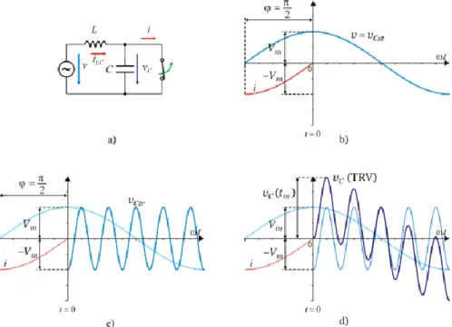
The circuit of Fig. 2.19 models a terminal fault, namely a short-circuit occurred at the terminals of a CB. There is no other component in the circuit between the switch and the fault. This and the circuit used for modeling switch-on (Fig. 2.2) are dissimilar in two points. First, the current model includes the resultant parallel capacitance C of the network, which plays a major role in determining the TRV. During calculation of the fault current, this C could be neglected, because – as 1/ω C>>ω L – the current through it has been very small. The other difference is that there is a resistance r parallel to the contacts of the CB in the model of Fig. 2.19. This r takes into account the resistance of the post-arc.
As a first approximation, we neglect the serial and parallel resistances in the model of Fig. 2.19, that is R=0, and r=∞. This damping - free model is shown in Fig. 2.20.a. It is worthy of notice, that the condition of R=0 is close to the reality of fault interruption in HV circuits, as cosυ≈0.1 there.
Fig. 2.20. Ideal switch-off of a fault in a solely inductive HV circuit
The moment of contact opening (t=0) coincides with the natural current zero of the steady-state prospective short-circuit current i. We assume that all switch-on transients has diminished by this time. We seek the voltage across the switch terminals after the time instant of switch-off. This voltage equals to the capacitor voltage v C(t).
Provided that 1/ω C>>ω L, after a long time, v C becomes identical to the supply voltage that is, v Cst(t)=v(t)=V
mcosω t. This voltage, the steady-state recovery voltage together with the prospective short-circuit current i lasted until its zero (t = 0) is plotted in Fig. 2.20.b. Since the circuit is solely inductive, this current lags behind the voltage by an angle of π/2. The picture clearly indicates that at t=0, v Cst(0)=V m. The capacitor voltage is the sum of two components in this case too:
(2-13)
We still do not know the transient time-function v Ctr(t), but we know that the capacitor voltage has been zero prior to switch-off, since the closed switch shunted out C. This voltage cannot jump, therefore its initial value is zero after current interruption, u C(0)=0. From these assumptions, the equation
(2-14)
follows, which results in v Ctr(0)=- V m. This is the initial value of the transient component, which is followed by a periodic oscillation caused by the current i LC in the L-C circuit of the network. There is no damping in the oscillation (R=0!), and its natural frequency
(2-15)
which is significantly higher (of the order of krad/s) than the angular frequency ω of the power supply. The time-function of the transient component (in other words oscillating component):
(2-16)
Switching transients
which starts with zero steepness. It is easy to verify that i LC(0)=0, as no current has been flowing in the L-C circuit before switch-off, and the current has been interrupted exactly in its natural zero. From this assumption:
(2-17)
consequently, just like v Cst, the initial slope of the resultant v C is zero (see Fig. 2.20c). It follows from this that the initial steepness of v Ctr is also zero.
Fig. 2.20.d shows the time-functions v Ctr(t) and v C (t), the latter one as the sum of v Ctr(t) and v Cst(t). The time- function v C (t) is the voltage appearing across the terminals of the switching device after the current interrupted, and it is called transient recovery voltage (TRV). In this case, the oscillation of the TRV has only one frequency: f 0=ω 0/2π.
The time-function of the TRV:
(2-18)
and its peak factor:
(2-19)
The peak factor is only slightly smaller than kp=2 – we can say that the difference is negligible – since the steady-state recovery voltage v Cst(t)=V mcosω t remains practically constant (V m) during a half cycle of the oscillating transient.
If we take into account the serial resistance R neglected previously, the phase shift between the fault current and the supply voltage will be less than π /2, although in HV circuits the difference from π /2 is usually negligible.
Not negligible however, is the damping of the oscillating part by a serial damping factor of
(2-20)
Besides, the natural frequency also changes, it will be slightly less than in the un-damped case:
(2-21)
Because of the lagging short-circuit current, of the reduced oscillation frequency, and above all, because of the damping, the peak factor of the TRV will be definitely less than 2.
Fig. 2.21. Ideal interruption of fault in a HV circuit with serial damping
Based on the previous assumptions, we can use a simplified, approximate formula to calculate the damped TRV after a fault interruption in an HV circuit:
TRV changes. On the one hand, its damping becomes stronger, since the resultant damping factor δ is the sum of a serial δ s and a parallel δ p part:
(2-23)
On the other hand, if the transient voltage is periodic, the difference between the damped and un-damped natural frequencies will not be negligible:
(2-24)
It is clear from this relation that the damped and un-damped oscillation frequencies can theoretically be equal, if δ p=δ s. In practice however, ω s<ω 0, since δ p>>δ s.
Again in favor of safety, we can use a simplified, approximate equation to calculate the TRV after a fault in a HV circuit with serial and parallel damping:
(2-25)
the plot of which is very similar to that of the serially damped case in Fig. 2.21.
3.2. Interruption of small inductive currents in HV circuits
Not only the high fault currents can cause problems during switch-off. Sometimes, the interruption of much smaller load currents can also be difficult, if the arc re-ignites after extinction. Two such cases exist. One of them is the breaking of capacitive load currents, like the switch-off of an idle overhead line or cable or a capacitor bank. Here we deal only with the other case, namely with the interruption of small inductive currents.
In practice, this can happen when switching off the no-load current of large transformers or medium voltage asynchronous motors, and it is dangerous only if the CB chops the arc current. Therefore we have to consider the arc voltage during the discussion of this phenomenon.
Fig. 2.22. Interruption of small inductive current; equivalent circuit
In Fig. 2.22, L 2 represents the inductance of an idle transformer, and C 2 its stray and interturn capacitances. The small inductance L 3 has a role only at re-ignition. The CB interrupts the current i at t=0 with chopping. The time-functions are plotted in Fig. 2.24, with the assumption that prior to interruption:
(2-26) and
Switching transients
(2-27)
and the difference of the two capacitor voltages provide the TRV after interruption.
Fig. 2.23. Interruption of small inductive current; time-functions
It can be observed in Fig. 2.23. that the voltage v 1 on the supply side tends to the supply voltage V m – considered as constant – with a damped oscillation of the frequency
(2-28)
The voltage v 1 continuously passes the moment of current break with the same steepness. The slope of the voltage v 2 is also continuous at this time instant, although v 2 oscillates around zero with the frequency of
(2-29)
and tends to zero with damping (ω 2<ω 1). The TRV starts from a finite value with a high steepness equal to that of the arc voltage; therefore it can easily re-ignite the arc. Assuming dielectric re-ignition, re-strike occurs at V 0, as it can be seen in Fig. 2.23. A high-frequency discharge current (i 3) starts to flow through the arc at this moment in the circuit of C 1 -L 3 -C 2 (see Fig. 2.22.). The resultant capacitance of two series connected capacitors:
(2-30)
which is charged to the voltage of V 0 at the moment of re-strike. Neglecting the losses, the energy stored in the capacitors is converted into the energy of the inductance L 3:
(2-31)
consequently the possible largest peak of the high-frequency discharge current:
(2-32)
and its angular frequency:
functions after a repeated chopping and re-ignition, and the final arc extinction on a smaller time-scale than in the previous figure. It is observable that the risk of re-ignition decreases toward the natural zero of the power- frequency current, as both the chopped current and the stored magnetic energy becomes smaller and smaller.
However, if re-strikes continue after the 50 Hz current zero, the chance of successful arc quenching will be less, the voltage gets higher, finally leading to sparkovers and probably to a short-circuit.
Fig. 2.24. Repeated re-ignition of arc current; time-functions
3.3. Interrupting a LV terminal fault
Fig. 2.25. Interruption of a terminal fault in a LV AC circuit; equivalent circuit
We have already mentioned in section 2.2.2.2 that the voltage of the short, non-linear switch arc is comparable to the supply voltage; it often surpasses the supply in LV systems. In an AC circuit this leads to the distortion of the prospective current, it will differ from sinusoidal. We will determine the time-function of the arc current i(t) from the approximate formula (2-9) of the arc voltage v arc (t) for an LV circuit modeling a terminal fault. The circuit is shown in Fig. 2.25. We will discuss the interruption with and without current limitation. Applying the principle of superposition will yield the current time-function i in both cases. At the moment of contact opening (t=0), a transient current i 2(t) begins to flow – due to the initiated arc voltage –opposite to the current i 1(t). The sum of these two currents results in the time-function we seek:
(2-34)
3.3.1. Interruption without current limitation
It can be observed in Fig. 2.26 that after fault occurrence, a prospective current i F flows until the moment of contact separation. We assume that this current is sinusoidal, although it can contain a DC component as well.
Contact separation happens only after the first current zero, therefore the peak of i F can evolve. The increase of the gap between the contact members raises the arc voltage, thus results in a more and more distorted and decreasing current i, compared to i F that would flow if the contacts remained closed. Probably more important is the shift of the current zeros. The zeros of i repeat each other more rapidly than that of i F. As a consequence, the steady-state recovery voltage will be smaller at these time instants, resulting in smaller initial value of the oscillating voltage and eventually in smaller TRV.
Switching transients
The voltage of the capacitor C cannot jump. As in reality, it has to decrease with a finite steepness. No matter if the TRV is periodic or aperiodic, after current zero, it must continue with the same slope. Therefore, to plot the TRV, we have to modify the arc voltage – originally described by (2-9) – in the short time interval close to the moment of interruption, as shown by the dashed line in Fig. 2.26. This modification has only a minor influence on the current, which cannot be observed in the figure.
Fig. 2.26. Interruption of a terminal fault without current limitation in an LV circuit; time- functions
If we take the current zero when the current passes from negative to positive as the moment of contact separation, then the time-function of the arc current up to its first zero:
(2-35)
where t s is the time instant of contact separation. This equation was obtained with the method of superposition.
Figure 2.26 illustrated a successful interruption, when the arc did not re-ignite after the second current zero, and the current remained steadily zero. We have seen in section 2.2.2.3 that, because of the strong de-ionizing and cooling effect of the relatively high mass electrodes, the primary cause of re-strike at low voltages is the spark breakdown. To examine re-ignition processes, we have to know the time-function of the ignition voltage v ign
appearing across the contact members (Fig. 2.15). Formula (2-10) provides a simple approximation of v ign. Figure 2.27 shows the example of an unsuccessful interruption, when the periodic TRV exceeded the re-ignition voltage, causing a re-strike.
Fig. 2.27. Unsuccessful interruption of a LV terminal fault, no current limitation
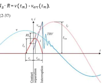
3.3.2. Interruption with current limitation
In case of current limiting circuit breakers, the peak I Fm of the prospective current i F cannot develop. The contacts open at a small momentary value of i F, and the arc voltage rises so fast that it soon exceeds the supply voltage. This effect is usually provoked by deion plates, discussed in chapter 6. It can be seen in Fig. 2.28 that the let-through current I lt, namely the limited peak, is less than I Fm, a merely 60 % of that. With real circuit breakers, we can expect even a much stronger effect; therefore it would not be illustrative to plot a real process
s F
differential equation
(2-36)
valid for the circuit of Fig. 2.25 yields the time function of the prospective current. The relation between the let- through current I lt and its time instant t m is easily derivable, as di/dt=0 at the moment of a t m:
(2-37)
Fig. 2.28. Interruption of a LV terminal fault with current limitation; time-functions
3. fejezet - Thermal transients
It is important to be familiar with the principles and basic calculation models of thermal processes taking place in equipment – like energy converters, conductors, switchgears and switching devices, etc. – of electric power systems. On the one hand, the ability to calculate temperature rise makes possible the economic design of the electrical apparatus without over-sizing. Inappropriate design can cause harmful overheating leading to operating failures. On the other hand, the operation of some of the electrical switching devices – like fuses, bi- metallic releases, thermal relays, etc. – is based on heating, and the operation of others – like circuit breakers, switches – is affected by the thermal effects of the electric arc.
The current flowing in the electrical conductors generates heat, namely thermal energy. One portion of this Joule-heat raises the temperature of the conductor, whereas another portion is transmitted to the environment.
During this transient thermal process, the conductor temperature ϑ (K) increases until it reaches steady-state, in other words heat balance. From this moment on, all the generated Joule-heat passes to the environment. Heat can be transferred on three different ways: heat conduction, thermal radiation and convection.
All the three heat transfer modes are taken into account in the heat transfer coefficient – or film coefficient – α (W/m2K) in the following equation:
(3-1)
where P (W) is the thermal power generated in the conductor, S (m2) is the heat transfer surface area, and τ is the difference in temperature between the surface ϑ (K) and the surrounding environment ϑ amb (K):
(3-2)
Table 3.1 compares the properties and possible mathematical simplifications of slow and fast thermal processes.
Operating and overload currents can cause slow, whereas short-circuits usually result in fast temperature rise.
Table 3.1.
Slow temperature rise
caused by operating and overload currents
Fast temperature rise caused by short-circuits
Most of the heat is transferred to the environment This condition is satisfied, if the duration of heating t h is of the same order of magnitude as the thermal time constant T h,.
The portion of heat transmitted to the environment is negligible. This condition is satisfied, if the duration of the fault t SC is much smaller than the thermal time constant (t SC T h).
The time of heating t h is much higher than the electrical time constant T of the circuits (t h T);
switch-on transients are negligible.
Switch-on transients can be negligible only if t SC T.
Temperature rise can be calculated with the rms value of the AC current.
Rms current value can be used for the calculations, only if switch-on transients are negligible that is t
SC T.
If only minor temperature rise occurs, then the temperature dependence of the electrical resistivity (ρ), the specific heat (c), and the film coefficient (α) are negligible that is, constant values can be used.
If the temperature rise is significant, then the temperature dependence of the electrical resistivity (ρ), the specific heat (c), and the film coefficient (α) have to be taken into account.