The Slow Demise of the Long-Lived SN 2005ip

The Slow Demise of the Long-Lived SN 2005ip

Ori D. Fox

, Claes Fransson

, Nathan Smith

, Jennifer Andrews

,

K. Azalee Bostroem

, Thomas G. Brink

, S. Bradley Cenko

, Geoffrey C. Clayton

, Alexei V. Filippenko

, Wen-fai Fong

, Joseph S. Gallagher

,

Patrick L. Kelly

, Charles D. Kilpatrick

, Jon C. Mauerhan

,

Adam M. Miller

, Edward Montiel

, Maximilian D. Stritzinger

, Tamás Szalai

, Schuyler D. Van Dyk

1Space Telescope Science Institute, 3700 San Martin Drive, Baltimore, MD 21218, USA.

2ofox@stsci.edu.

3Department of Astronomy, Oskar Klein Centre, Stockholm University, AlbaNova, SE–106 91 Stockholm, Sweden.

4Steward Observatory, 933 N. Cherry Ave., Tucson, AZ 85721, USA.

5Department of Physics, University of California, Davis, CA 95616, USA.

6Department of Astronomy, University of California, Berkeley, CA 94720-3411, USA.

7NASA Goddard Space Flight Center, 8800 Greenbelt Road, Greenbelt, DMD 20771, USA.

8Joint Space-Science Institute, University of Maryland, College Park, MD 20742, USA.

9Dept. of Physics & Astronomy, Louisiana State University, Baton Rouge, LA 70803, USA.

10Miller Senior Fellow, Miller Institute for Basic Research in Science, University of California, Berkeley, CA 94720, USA.

11Center for Interdisciplinary Exploration and Research in Astrophysics (CIERA) and Department of Physics and Astronomy, Northwestern University, Evanston, IL 60208, USA.

12University of Cincinnati Blue Ash College, 9555 Plainfield Rd., Blue Ash, OH 45236, USA.

13Minnesota Institute for Astrophysics, University of Minnesota, 115 Union St. SE, Minneapolis, MN 55455, USA.

14Department of Astronomy and Astrophysics, University of California, Santa Cruz, CA 95064, USA.

15The Aerospace Corporation, 2310 E. El Segundo Blvd., El Segundo, CA 90245, USA.

16Jet Propulsion Laboratory, 4800 Oak Grove Drive, MS 169-506, Pasadena, CA 91109, USA.

17California Institute of Technology, Pasadena, CA 91125, USA.

18Hubble Fellow.

19SOFIA-USRA, NASA Ames Research Center, Mail Stop N232-12, Moffett Field, CA 94035-1000, USA.

20Department of Physics and Astronomy, Aarhus University, Ny Munkegade 120, DK-8000 Aarhus C, Denmark 21Department of Optics and Quantum Electronics, University of Szeged, H-6720 Szeged, Dóm tér 9., Hungary.

22Konkoly Observatory, Research Centre for Astronomy and Earth Sciences, H-1121 Budapest, Konkoly Thege Miklós út 15-17, Hungary.

23IPAC/Caltech, Mailcode 100-22, Pasadena, CA 91125, USA.

7 August 2020

ABSTRACT

The Type IIn supernova (SN) 2005ip is one of the most well-studied and long-lasting ex- amples of a SN interacting with its circumstellar environment. The optical light curve plateaued at a nearly constant level for more than five years, suggesting ongoing shock interaction with an extended and clumpy circumstellar medium (CSM). Here we present continued observa- tions of the SN from∼1000−5000 days post-explosion at all wavelengths, including X-ray, ultraviolet, near-infrared, and mid-infrared. The UV spectra probe the pre-explosion mass loss and show evidence for CNO processing. From the bolometric light curve, we find that the total radiated energy is in excess of 10⁵⁰erg, the progenitor star’s pre-explosion mass-loss rate was

∼>1×10⁻²Myr⁻¹, and the total mass lost shortly before explosion was >

∼1 M, though the mass lost could have been considerably larger depending on the efficiency for the conversion of kinetic energy to radiation. The ultraviolet through near-infrared spectrum is characterised by two high density components, one with narrow high-ionisation lines, and one with broader low-ionisation H I, He I, [O I], Mg II, and Fe II lines. The rich Fe II spectrum is strongly affected by Lyαfluorescence, consistent with spectral modeling. Both the Balmer and He I lines indicate a decreasing CSM density during the late interaction period. We find similarities to SN 1988Z, which shows a comparable change in spectrum at around the same time during its very slow decline. These results suggest that, at long last, the shock interaction in SN 2005ip may finally be on the decline.

Key words: circumstellar matter — supernovae: general — supernovae: individual (SN 2005ip) — dust, extinction — infrared: stars

arXiv:2008.02301v1 [astro-ph.HE] 5 Aug 2020

2

1 INTRODUCTION

Type IIn supernovae (SNe IIn; seeFilippenko 1997andSmith 2017 for reviews) are characterised by relatively narrow emission lines (Schlegel 1990) which are not associated with the SN explosion itself, but rather with dense circumstellar material (CSM) produced by pre-SN mass loss (Smith 2014). Shock interaction and dust for- mation in the dense CSM often result in significant emission ranging from X-ray to radio wavelengths for many years post-explosion (e.g., Chevalier & Fransson 2017;Fox et al. 2011,2013).

SN 2005ip, discovered in NGC 2906 (Boles et al. 2005) on 2005 November 5.163 (UT dates are used throughout this paper), is one of the more well-studied Type IIn explosions given its proxim- ity to Earth (∼35 Mpc) and the fact that it has remained detectable for nearly 15 years post-explosion.Fox et al.(2009) first reported a 3 yr near-infrared (NIR) light-curve plateau corresponding to newly formed dust in the cold, post-shock shell.Smith et al.(2009b) pub- lished an optical light curve that showed an initial linear (in mag d⁻¹) decline from peak, followed by a late-time plateau attributed to on- going shock interaction with the dense CSM. The late optical plateau matched the NIR plateau, andSmith et al.(2009b) presented spec- tra that revealed signatures of strong ongoing CSM interaction, as well as signatures of dust formation in both the SN ejecta and the post-shock cold dense shell. SN 2005ip was unusual in displaying very pronounced narrow coronal emission lines in its spectrum, in- dicating that clumpy CSM was being strongly irradiated by X-rays from the shock interaction (Smith et al. 2009b). Coronal lines have also been seen in the Type IIn SNe 1995N (Fransson et al. 2002), 2006jd (Stritzinger et al. 2012), and SN 2010jl (Fransson et al.

2014).Fox et al.(2010) obtained aSpitzer Space TelescopeInfrared Spectrograph (IRS;Houck et al. 2004) spectrum of SN 2005ip (the only mid-IR (MIR) spectrum of a SN IIn to date), which revealed the presence of a second, cooler dust component associated with a pre-existing dust shell radiatively heated by this ongoing CSM interaction.Bevan et al.(2018) modeled the spectral line evolution and confirmed that a significant amount of dust can be explained by dust formation in the ejecta, andNielsen et al.(2018) found the dust properties to be unlike those of Milky Way dust.

Stritzinger et al. (2012) continued to monitor SN 2005ip throughout∼5 yr post-explosion and showed that the optical and NIR light curves underwent little decline over that time.Katsuda et al. (2014) reported that X-ray observations at ∼ 6 yr post- explosion exhibit a significant decrease in flux compared to previous epochs, suggesting the forward shock had finally overtaken the dense CSM in which the SN exploded. Most recently,Smith et al.(2017) observed a temporary resurgence in the Hαluminosity, which they interpreted to be the result of the forward shock crashing into an additional dense shell located.0.05 pc away, consistent with the distant pre-existing dust shell indicated by MIR observations (Fox et al. 2011). Overall,Smith et al.(2017) showed that the spectral evolution and X-ray emission from the decade-long CSM interac- tion phase of SN 2005ip was almost identical to the late interaction seen in SN 1988Z, the prototypical SN IIn with long-lasting CSM interaction.

The nature of the progenitors of both SN 2005ip and the broader Type IIn subclass remains ambiguous. The mass-loss rates of SNe IIn derived using various techniques are in the range 10⁻⁴– 10⁻¹M yr⁻¹ and the total CSM masses are several M (e.g., Smith et al. 2009b,2007,2008;Fox et al. 2009;Moriya et al. 2013;

Ofek et al. 2014;Fransson et al. 2014;Katsuda et al. 2014;Smith 2017). Galactic analogs with such mass-loss rates and H-rich winds include luminous red supergiants, yellow hypergiants, and luminous

blue variables (LBVs), each of which present further questions of their own (seeSmith 2014for a review). To complicate the inter- pretation even more,Habergham et al.(2012) find that SNe IIn, including SN 2005ip, do not trace the most active star formation in galaxies, suggesting they are not exclusively associated with the most massive stars.Smith & Tombleson(2015) note that extremely luminous LBVs themselves do not trace regions of recent massive star formation, and go on to explain this effect with a binary pro- genitor scenario.Nomoto et al.(1995) also stressed the importance of binary evolution in various types of SN progenitors including SNe IIn. On the other hand, SNe IIn share many properties with SN impostors (Smith et al. 2011), and pre-existing dust shells are reminiscent of the impostors’ pre-SN eruptions, such as SN 2009ip (e.g.,Mauerhan et al. 2013), where the eruption was linked to an LBV progenitor (e.g.,Smith et al. 2010).Taddia et al.(2015) find that long-lasting SNe IIn have similar host-galaxy metallicities as SN imposters, which may be produced by LBV outbursts and have traditionally been thought to arise from massive stars.

The pre-SN mass-loss history of SNe IIn may hold some clues since it probes the latest stages of massive-star evolution. Differ- ences in wind speeds, densities, compositions, and asymmetries result in distinguishable observational behaviours. Given the dense CSM associated with most SNe IIn, X-rays from shock interaction are often absorbed, reprocessed, and re-emitted at UV (predomi- nantly) and optical wavelengths, making these wavelengths optimal for tracing CSM interaction and, thereby, the progenitor’s mass-loss history (e.g.,Chevalier & Fransson 1994;Chevalier & Irwin 2011;

Chevalier & Fransson 2017). Furthermore, when combined with other wavelengths, the UV may offer a quantitative estimate of the nucleosynthesis in the core of the star, which helps to constrain the initial mass of the progenitor prior to mass loss (Fransson et al.

2002,2005,2014).

Here we present multiwavelength observations of SN 2005ip at very late epochs, including UV, optical, NIR, MIR, and radio.

These data track the SN light curve as it declines in all bands.

FollowingStritzinger et al.(2012), throughout this paper we assume that the distance to NGC 2906 (the host galaxy) is 34.9 Mpc, and we adoptE(B−V)=0.047 mag as the reddening (Smith et al. 2009b).

When noted, we correct our spectral energy distributions (SEDs) and spectra for this colour excess assumingR_V=A_V/E(B−V)= 3.1 using the reddening law of Cardelli et al.(1989). Section2 presents the observations, while §3analyzes the light curve and spectral evolution. In §3.2.3we take a closer look at the UV spectra.

Finally, §4provides a discussion and conclusion of the work.

2 OBSERVATIONS 2.1 HSTImaging

Table1 summarisesHubble Space Telescope (HST) imaging of SN 2005ip. We obtained individual images from the Mikulski Archive for Space Telescopes (MAST), so they have been pro- cessed through the standard pipeline at the Space Telescope Sci- ence Institute (STScI). We obtained photometry from individual flc frames using Dolphot (Dolphin 2016) with the following param- eters: FitSky=3, RAper=8, and InterpPSFlib=1, and the TinyTim model point-spread functions (PSFs).

Table 1.HSTImaging

UT Date Epoch Program PI Instrument Grating/Filter Central Wavelength Exposure Magnitude

YYYMMDD (d) (GO) (Å) (s)

20081118 1109 10877 Weidong Li WFPC2 F450W 4556.00 800 19.58 (0.01)

20081118 1109 10877 Weidong Li WFPC2 F675W 6717.00 360 17.30 (0.01)

20081118 1109 10877 Weidong Li WFPC2 F555W 5439.00 460 19.34 (0.01)

20081118 1109 10877 Weidong Li WFPC2 F814W 8012.00 700 19.05 (0.01)

20161029 4011 14668 Filippenko WFC3 F336W 3354.85 780 20.82 (0.02)

20161029 4011 14668 Filippenko WFC3 F814W 8048.10 710 21.31 (0.01)

20180111 4450 15166 Filippenko WFC3 F336W 3354.85 780 21.32 (0.02)

20180111 4450 15166 Filippenko WFC3 F814W 8048.10 710 21.60 (0.01)

Table 2.HST/STIS/MAMA Spectroscopy

UT Date Epoch Program Grating Exposure

YYYYMMDD (d) (GO) (s)

20140328 3065 13287 G140L 4752

G230L 2744

20171021 4368 14598 G140L 17,100

G230L 19,008

2.2 HST/STIS

SN 2005ip was observed twice with theHST/STIS as part of pro- grams GO-13287 and GO-14598 (PI O. Fox), as summarised in Table2. The one-dimensional (1D) spectrum for each observation is extracted using the CALSTIS custom extraction software stis- tools.x1d. The default extraction parameters for STIS are defined for an isolated point source. For both G140L and G230L the default extraction box width is 7 pixels and the background extraction box width is 5 pixels.

2.3 WarmSpitzer/IRAC Photometry

The Warm Spitzer Infrared Array Camera (IRAC) (Fazio et al.

2004) obtained several epochs of data for SN 2005ip, summarised in Table3and plotted in Figure1. We downloaded coadded and cal- ibrated Post Basic Calibrated Data (pbcd) from theSpitzerHeritage Archive. Standard aperture photometry was performed with a radius defined by a fixed multiple of the PSF full width at half-maximum intensity (FWHM). Template subtraction is typically implemented to remove contributions from the underlying galaxy, but in this case, noSpitzertemplate exists. Furthermore, due to the rapid flux vari- ations of the underlying galaxy, a standard annulus does not allow for selection of pixels corresponding to a local background associ- ated with the SN (e.g.,Fox et al. 2011;Szalai et al. 2019). Instead, we selected our own background region. The standard deviation of the background variations is smaller than the measured noise in the aperture photometry, even at the latest epochs, and does not contribute substantially to our error bars. Most of these data were recently published bySzalai et al.(2019), but day 4667 is newly published here. The photometry for epochs 948 and 2057 doesn’t precisely match the photometry ofFox et al.(2010,2011,2013) because the analysis in those papers implemented slightly different routines consisting of either different sized apertures or PSF fitting photometry, but they are within the error bars. AllSpitzerphotom- etry in this paper was calculated using aperture photometry with consistent aperture sizes.

For plotting purposes in Figure1, we derive the integrated

Table 3.S pitzerPhotometry

JD− Epoch PID 3.6µm 4.5µm

2,450,000 (d) (10¹⁷erg s⁻¹cm⁻²Å⁻¹) 4628 948 50256 13.62(0.31) 10.96(0.21) 5737 2057 80023 6.44(0.20) 5.87(0.15) 6476 2796 90174 3.36(0.15) 3.02(0.11) 6845 3165 10139 2.68(0.14) 2.32(0.09) 7229 3549 11053 2.22(0.13) 1.80(0.08) 8347 4667 14098 1.56(0.11) 1.05(0.07)

Spitzerluminosity by fitting a simple dust-mass model to the two MIR data fluxes, similar to those described byFox et al.(2011).

In this case, we assume 0.1µm graphite grains given the lack of the∼10µm silicate feature in the MIR spectrum (Fox et al. 2010;

Williams & Fox 2015).

2.4 Optical and NIR Photometry

Tables4and 5list and Figure 1plots the new optical and NIR photometry of SN 2005ip. We include some data obtained with the Reionization And Transients InfraRed camera (RATIR;Butler et al. 2012;Fox et al. 2012) mounted on the 1.5 m Johnson telescope at the Mexican Observatorio Astrono ´mico Nacional on Sierra San Pedro Mártir in Baja California, México (Watson et al. 2012). The data were reduced, coadded, and analysed using standard CCD and IR processing and aperture photometry techniques, utilising online astrometry programsSExtractorandSWarp¹.

We also present two epochs ofr andiphotometry obtained during 2014 at Las Campanas Observatory with the 2.5 m du Pont telescope by the Carnegie Supernova Project (CSP;Hamuy et al.

2006). These images were reduced following standard procedures.

PSF photometry of the SN was computed in the natural system using the local sequence stars presented byStritzinger et al.(2012). The reported photometric uncertainties account for both instrumental and nightly zero-point errors.

Additional NIR photometry was obtained from the 3.8 m United Kingdom Infrared Telescope (UKIRT) on Maunakea using WFCAM2.J HKobservations were pipeline reduced by the Cam- bridge Astronomical Survey Unit (CASU). Aperture photometry was performed using the DAOPHOT package inIRAF². Uncertain-

1 SExtractor and SWarp can be accessed from

http://www.astromatic.net/software.

2 IRAF: the Image Reduction and Analysis Facility is distributed by the Na- tional Optical Astronomy Observatory, which is operated by the Association 000

4

Table 4.Ground-Based Optical Photometry

JD− Epoch g⁰ B V R r I i Instrument

2,450,000 (d) mag

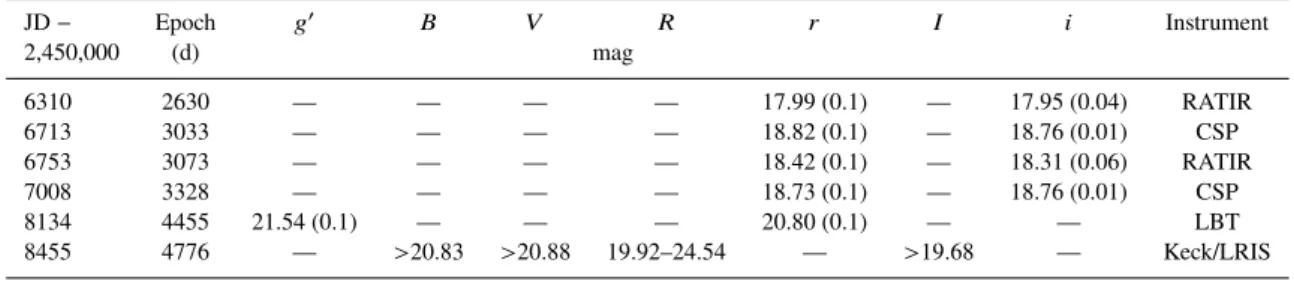
6310 2630 — — — — 17.99 (0.1) — 17.95 (0.04) RATIR

6713 3033 — — — — 18.82 (0.1) — 18.76 (0.01) CSP

6753 3073 — — — — 18.42 (0.1) — 18.31 (0.06) RATIR

7008 3328 — — — — 18.73 (0.1) — 18.76 (0.01) CSP

8134 4455 21.54 (0.1) — — — 20.80 (0.1) — — LBT

8455 4776 — >20.83 >20.88 19.92–24.54 — >19.68 — Keck/LRIS

Table 5.Ground-Based NIR Photometry

JD− Epoch Z Y J H K Instrument

2,450,000 (d) mag

6310 2630 17.47 (0.01) — 16.27 (0.01) 15.65 (0.02) — RATIR

6753 3073 17.91 (0.01) — 16.77 (0.02) 16.09 (0.02) — RATIR

7435 3755 — — 19.81 (0.1) 18.91 (0.1) 17.3 (0.1) UKIRT

7451 3771 — — — — 17.2 (0.1) UKIRT

7483 3803 — — — 18.96 (0.1) 17.2 (0.1) UKIRT

ties were calculated by adding in quadrature photon statistics and zero-point deviation of the standard stars for each epoch.

One epoch ofg0and r0photometry was obtained with the Multi-Object Double Spectrograph (MODS; Byard & OâĂŹBrien 2000) on the Large Binocular Telescope (LBT) on 2018 January 16. The 3×240 s images in each filter were reduced and stacked using standardIRAFprocedures, and zero points were calculated using Sloan Digital Sky Survey (SDSS) standard stars in the field.

Uncertainties were calculated in the same manner as for the UKIRT data.

All magnitudes were initially calculated in their respective tele- scopes natural system. Although not every telescope has a published report detailing their system, they all follow similar techniques as CSP (Contreras et al. 2010). All photometric calibration was then performed using field stars with reported fluxes in both 2MASS (Skrutskie et al. 2006) and the SDSS Data Release 9 Catalogue (Ahn et al. 2012). Uncertainties are dominated by errors associated with catalog stars.

The most complicated point in Figure1is the 2018R-band photometry from Keck (day 4776), when the SN is quite faint and comparable in broad-band flux to the underlying H II region. Aper- ture photometry, which includes some of the underlying H II region, yields a magnitude of 19.92, which we take to be the SN upper limit (Table4). We also obtained a final epoch of KeckR-band imaging in 2019. Under the assumption that the SN had faded completely (although it likely hadn’t), we can use the 2019 data as a template for subtraction from the 2018 data. This yields a magnitude of 24.54, which we take to be the SN lower limit in 2018. In reality, the actual SN flux on day 4776 is somewhere between these limits.

2.5 Optical Spectroscopy

Table 6 lists and Figure2 plots the new optical spectra of SN 2005ip. We obtained some spectra with the Low Resolution Imag- ing Spectrometer (LRIS;Oke et al. 1995) mounted on the 10 m

of Universities for Research in Astronomy (AURA), Inc., under cooperative agreement with the US National Science Foundation (NSF).

Table 6.Ground-Based Spectroscopy

JD− Epoch Instrument Res. Exp.

2,450,000 (d) (Å) (s)

4584 905 Keck/LRIS ∼9 1200

6246 2567 Keck/DEIMOS ∼3 2400

6778 3099 Keck/LRIS ∼6 1200

7372 3693 Keck/DEIMOS ∼3 2400

7449 3770 Keck/DEIMOS ∼3 2400

7893 4214 MMT/BC ∼1 1200

8052 4373 MMT/BC ∼1 1200

8109 4430 MMT/BC ∼1 1200

8784 5105 Keck/LRIS ∼6 1200

Keck I telescope and the DEep Imaging Multi-Object Spectrograph (DEIMOS;Faber et al. 2003) mounted on the 10 m Keck II tele- scope. For the Keck/LRIS spectra, we observed with a 1⁰⁰wide slit and used either the 600/4000 or 400/3400 grisms on the blue side and the 400/8500 grating on the red side. This observing setup resulted in wavelength coverage from 3200–9200 Å and a typical resolution of 5–7 Å. For the Keck/DEIMOS spectra, we observed with a 1⁰⁰wide slit and the 1200/7500 grating. This observing setup resulted in wavelength coverage from 4750–7400 Å and a typical resolution of∼3 Å. In both cases, we aligned the slit the paral- lactic angle to minimise differential light losses (Filippenko 1982).

These spectra were reduced using standard techniques (e.g.,Foley et al. 2003;Silverman et al. 2012). Routine CCD processing and spectrum extraction were implemented using the optimal algorithm ofHorne(1986). We flux calibrated these spectra and removed tel- luric absorption lines using alagorithms defined byWade & Horne (1988) andMatheson et al.(2000).

We also obtained three epochs of spectroscopy with the Bluechannel (BC) spectrograph on the 6.5 m Multiple Mirror Tele- scope (MMT) using the 1200 l mm⁻¹ grating centred at 6300 Å (seeSmith et al. 2017). We performed standard reductions, includ- ing bias subtraction, flat-fielding, and optimal spectral extraction.

We flux calibrated these spectra using spectrophotometric standards observed at similar airmasses.

2.6 Chandra X-Ray Photometery

TheChandra X-ray Observatory(CXO) Advanced CCD Imaging Spectrometer (ACIS; Garmire et al. 2003) observed SN 2005ip, summarised in Table 7and plotted in Figure1. As a reference, we also include details of the previous epoch of CXO obser- vations from 2016 (Smith et al. 2017). Similar to Smith et al.

(2017), we performed photometry and spectral extraction using thespecextractpackage within the HEASOFT³Ciaosoftware suite (Blackburn 1995). We model source and background spectra simultaneously using theSherpapackage. For the source, we as- sume an absorbed single-temperature thermal plasma model (apec) having solar abundances as defined byAsplund et al.(2009). For the background, we assume a simple power law. We set the equiv- alent neutral hydrogen column density in the interstellar medium (ISM) ofN_H(ISM) =3.7×10²⁰cm⁻²(Katsuda et al. 2014). We also allowed for an additional intrinsic source of absorption for the SN. The fits rely on aχ²statistic with a Gehrels variance function.

In this case, we obtained a reduced χ²value of 35 for 64 degrees of freedom. We use these fits to derive photon energies in the range 0.5–8.0 keV. Compared to our previously reportedChandra/ACIS observation on 2016 Apr. 3 (Smith et al. 2017), SN 2005ip exhibits a factor of∼2 reduction in the intrinsic flux. The temperature and self-absorption parameters of our thermal plasma model, however, have not changed significantly.

3 ANALYSIS

3.1 Light-Curve Evolution, Bolometric Luminosity, and Radiated Energy

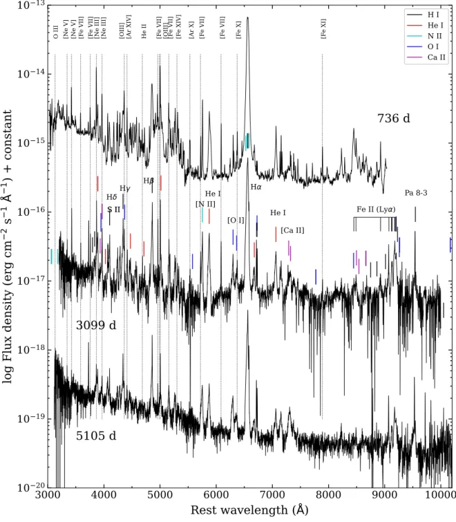
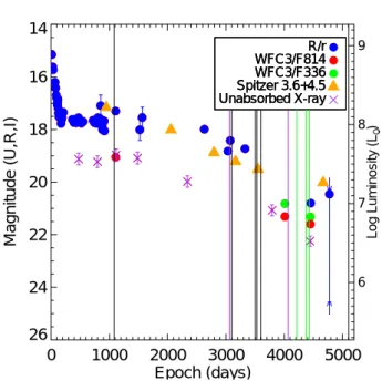
Figure1shows decreasing fluxes at all wavelengths at days&1500 post-explosion, which is consistent with other SNe IIn observed at such late epochs (Fox et al. 2011). Based on the X-ray observations alone, Katsuda et al. (2014) attribute the decreasing flux to the forward shock having finally overtaken the dense CSM in which the SN exploded. Figure2shows that most of the decreasing flux occurs in the strength of Hαline, although the later spectra suggest that there may be some additional contribution from outside the Hα line, possibly from a faint reflected light echo or a blend of very faint CSM interaction lines and their wings.

We use the data from Figure1to construct a quasibolometric luminosity light curve (Figure3), which we will refer to simply as the bolometric light curve hereafter. For the optical, we use ourr- band photometry and scale magnitudes to correspond to the optical luminosities fromStritzinger et al.(2012) in the range 350–900 d, assuming that the spectrum does not change appreciably after this epoch. This includes both the “hot" component and the lines in Stritzinger et al.(2012), giving

L_optical=10^{−0.4r+48.45}. (1)

The IR luminosities are described above. The MIR luminosities do not include the cold component discussed byFox et al.(2010), whose origin may be from more distant gas. Taken all together, the bolometric luminosity may be underestimated by at most 50%.

Because we do not include the far-IR, UV, or X-rays, this is likely to be a lower limit to the luminosity. The observed X-rays give an additional contribution of (15%–20%). Unfortunately, this compo- nent is not known before 460 d. For the total bolometric output only

3 http://heasarc.gsfc.nasa.gov/ftools

0 1000 2000 3000 4000 5000 Epoch (days)

26 24 22 20 18 16 14

Magnitude (U,R,I)

R/r WFC3/F814 WFC3/F336 Spitzer 3.6+4.5 Unabsorbed X-ray

6 7 8 9

Log Luminosity (LO •) R/r WFC3/F814 WFC3/F336 Spitzer 3.6+4.5 Unabsorbed X-ray R/r WFC3/F814 WFC3/F336 Spitzer 3.6+4.5 Unabsorbed X-ray

Figure 1.Multiwavelength photometry of SN 2005ip, including data pre- sented in this paper,Smith et al.(2009b),Fox et al.(2010),Stritzinger et al.

(2012),Katsuda et al.(2014), andSzalai et al.(2019). Vertical identify epochs on which the spectra presented here were obtained (black=Keck, green=MMT, and purple=Chandra). Note that the left ordinate axis applies only to theR/r band, F814, and F336 photometry, while the right-hand ordinate axis applies to theSpitzerintegrated and X-ray luminosities. The most complicated point in Figure1is the 2018R-band photometry from Keck (day 4776), when the SN is quite faint and comparable in broad-band flux to the underlying H II region. Aperture photometry, which includes some of the underlying H II region, yields a magnitude of 19.92, which we take to be the SN upper limit (Table4). We also obtained a final epoch of KeckR-band imaging in 2019. Under the assumption that the SN had faded completely (although it likely hadn’t), we can use the 2019 data as a template for subtraction from the 2018 data. This yields a magnitude of 24.54, which we take to be the SN lower limit in 2018. In reality, the actual SN flux on day 4776 is somewhere between these limits.

the observed X-ray luminosity should be included, not the fraction absorbed by the CSM, which is thermalised into UV and opti- cal radiation. This fraction is most likely increasing for the earlier epochs, approaching 100% as the column density of the CSM and ejecta ahead of the shock increases at early epochs. This is highly model dependent, and we do therefore not attempt to model it. To estimate the effect, however, we add the observed X-ray luminosity to the optical and IR contributions, shown as the dashed black line in Figure3.

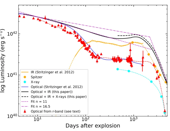
Figure3shows that the optical plus IR luminosity up to∼ 700 d can be well described by a power law in time, L ≈ 2.6× 10⁴²(t/(10 d))^−0.33erg s⁻¹. The power-law decay during the first phase can be well described by the similarity solution for a radiative shock in a CSM with a steady mass-loss rate (e.g., Chevalier &

Fransson 2017): L ∝ v_s³ ∝ t^−3/(n−2), wherenis the power-law index of the ejecta density profile. If we use only the total optical plus IR light curve, the luminosity decrease corresponds ton≈11, somewhat steeper than found for SN 2010jl (Fransson et al. 2014).

When we also include the X-rays, the dip in the optical plus IR light curve before the plateau partly fills in, increasing the luminos- ity by∼20%. If we fit the luminosity from 10 d to the peak of the 000

6

Table 7.ChandraObservations of SN 2005ip

Instrument JD− Days After Exposure Counts N_H kT 0.5–8 keV Luminosity

2,450,000 Outburst (ks) (10⁻³ (10²² (keV) Unabsorbed Flux (10⁻¹³ (10⁴⁰erg s⁻¹) counts s⁻¹) cm⁻²) erg s⁻¹cm⁻²)

ACIS-S 7482 3812 35.59 820 0.19^+0.08_−0.07 5.0^+1.1_−0.9 2.86^+0.12_−0.08 3.2 ACIS-S 8122 4453 41.22 619 0.11^+0.25−0.11 3.2^+2.0−1.2 1.2^+1.0−1.1 1.3

4000 5000 6000 7000 8000 9000 10000

Rest-Frame λ (Ang) -22

-20 -18 -16

Log (erg s-1 cm-2 Ang-1 )

4000 5000 6000 7000 8000 9000 10000

Rest-Frame λ (Ang) -22

-20 -18 -16

Log (erg s-1 cm-2 Ang-1 )

20080428 (day 905)+0.

20140501 (day 3099)-1.0 20151216 (day 3693)-1.7 20160302 (day 3770)-3.9 20191028 (day 5105)-4.0

Figure 2.Some of the ground-based optical spectra summarised in Table6. The spectra are scaled to the optical photometry for absolute comparisons at each epoch.

“bump" at∼1000 d, we findL≈2.6×10⁴²(t/(10 d))^−0.21erg s⁻¹, corresponding ton=16.5. Note, however, that this excludes any X-ray contribution at earlier epochs which would steepen the de- cline and decreasen. In this context we also note that a short-lived eruption, as is probably the case here, may have a density profile different from a steadyρ∝r⁻²wind.

After∼2000 d the light curve breaks, and the decay is steeper, withL ∝ (t/(10 d))⁻³. This behaviour signals the breakout of the shock wave from at least part of the dense CSM. Compared again to SN 2010jl, where the break occurred at∼350 d, this is considerably later.

We integrate the bolometric light curve to estimate a total radiated energy of 1.7×10⁵⁰erg. We add∼1×10⁴⁹erg from the X-rays. As we discuss above, however, this is most likely only a lower limit to the total radiated energy.

Using the bolometric light curve we can also estimate the mass-loss rate. Assuming a radiative shock in a steady wind, the

total luminosity is given by L=1

2MÛ v_wv³

shock, (2)

where ≤ 1 is the efficiency for conversion,v_shock is the shock velocity,MÛ is the mass-loss rate, andv_wis the wind velocity. From the narrow high-ionisation lines we estimate the velocity of the pre- shocked CSM to be∼100 km s⁻¹. If we write the luminosity as L(t)=L(t∗)(t/t∗)^αandv_shock=v_shock(t₀/t)^1/(n−2), we get MÛ = 2L(t∗)v_w

v_shock(t₀)³ t∗

t_{0 3}/(n−2)

. (3)

The shock velocity injects the largest uncertainty in the above equation. Because of electron scattering at early epochs, one can- not use the maximum wavelength shift of the blue wing. Figure 6 ofSmith et al. (2009b) shows that this line has a “shoulder"

at∼ 5300 km s⁻¹ on the blue side in the spectra at∼100 d. As discussed in detail byTaddia et al.(2020), this shoulder may be caused by the macroscopic shock velocity, in contrast to the wings

10 ¹ 10 ² 10 ³

Days after explosion

10 ⁴⁰ 10 ⁴¹ 10 ⁴²

log Luminosity (erg s −1 )

IR (Stritzinger et al. 2012) Spitzer

X-ray

Optical (Stritzinger et al. 2012) Optical + IR (this paper))

Optical + IR + X-rays (this paper) Fit n = 11

Fit n = 16.5

Optical from r-band (see text)

Figure 3.Quasibolometric light curve of SN 2005ip. The solid lines are the optical (blue) and IR (orange) light curves fromStritzinger et al.(2012), while the dashed lines are fits to ther-band (red) andSpitzer(orange) light curves, with photometry from this paper. The solid black line is the total constructed by merging the light curves fromStritzinger et al.(2012) and this paper. The dashed magenta lines show power-law fits to the two phases of the total luminosity (including and excluding X-rays, which are shown in cyan).

caused by electron scattering. Our late-time Hαspectra (Sec.3.2.4) indicate a velocity of∼2700 km s⁻¹at∼1000 d, but the line pro- file still suggests contributions from electron scattering. Given this uncertainty, we will therefore scale the mass loss to a velocity of 3000 km s⁻¹at 1000 d, as in Eq.4.

Witht∗ =10 d,L(t∗) =2.6×10⁴²erg s⁻¹, andt₀ =1000 d, we get

MÛ =6.6×10⁻³

v_w 100 km s⁻¹

v_shock(1000 d) 3000 km s⁻¹

−3

Myr⁻¹. (4) The total mass of the SN 2005ip gas shell up to the break att_break is then

Mtot=MÛ

v_wv_shock(t₀)t_break t₀

t_{break 1}/(n−2)

. (5)

If we assume that the shock has exited the densest part of the CSM att_break≈2000 d and withMÛ from Eq.4, we get

Mtot=1.0

v_shock(1000 d) 3000 km s⁻¹

−2 t_break 2000 d

8/9

M. (6)

Equations 4 and 6 together give a timescale of ∼ 150(v_shock(1000 d)/3000 km s⁻¹) (v_w/100 km s⁻¹)⁻¹ yr for the strong mass-loss episode.

If we instead use the flatter evolution of the luminosity in Figure3withn = 16.5, the coefficient in Eq.4becomes 1.2× 10⁻²Myr⁻¹, and in Eq.6the coefficient becomes 1.85M.

As seen from Eqs.4and 6, besides the value of v_shock, an important uncertainty in these estimates is the efficiency parameter, , which depends on the importance of shock-wave instabilities and other multidimensional effects (Taddia et al. 2020), and may be in the range∼0.1–1. For these reasons, the total radiated energy and total mass should be taken as lower limits. In addition, we only integrated the total mass swept to the break at∼2000 d. Even if the light-curve steepening is caused by a decreasing density, the later evolution will certainly contribute to a substantial additional mass.

Other studies using X-ray and MIR data favour total CSM masses even higher than 10 M (Stritzinger et al. 2012;Katsuda et al. 2014). These results are consistent with mass-loss rates that are all nearly 10⁻²Myr⁻¹for a period of several hundred years leading up to the progenitor’s explosion, similar to what we find 000

8

above. The superluminous Type IIn SN 2010jl, for comparison, had a mass-loss rate of nearly 10⁻²Myr⁻¹and total mass loss of

&3 M.

3.2 Spectral Modeling and Line Identifications

Basic modeling can be used to infer some qualitative estimates of the physical conditions in the CSM and SN, although this should not be confused with a fully self-consistent spectral modeling (e.g., Dessart et al. 2015). Already, there has been extensive discussion of the rich line spectra of SN 2005ip (Smith et al. 2009b;Smith et al.

2017;Stritzinger et al. 2012). The H I, He I, [N II], [O I], Mg II, and [Ca II] lines have FWHM≈1500 km s⁻¹and are understood to originate from a denser, optically thick medium. We will refer to these as the low-ionisation component. In contrast, the high- ionisation lines are all narrow, originating in the preshocked CSM with FWHM≈350 km s⁻¹.

3.2.1 Low-ionisation lines and Lyαfluorescence

As a tool for line identifications and for the diagnostics we have calculated a synthetic spectrum, including H I, He I, N II, O I, Mg II, Ca II, and Fe II, which account for most of the spectral features.

For H I, He I, N II, O I, and Fe VII, we use multilevel model atoms, including collisional and radiative processes. We assume a two-zone model with temperature and density as parameters: one zone for the neutral and singly ionised elements and one zone for the high-ionisation ions. We include optical-depth effects for the lines in the Sobolev approximation. The ionic abundances are treated as parameters. The atomic data for high-ionisation stages are from the CHIANTI database (Landi et al. 2012). For H I we use collision rates fromAnderson et al.(2002) and for He I fromBenjamin et al.

(1999). Radiative transition rates and energy levels are mainly from NIST.

We have not attempted a similar calculation for Fe II, in spite of the large number of lines in the spectrum. This requires a more detailed calculation, including radiative excitation by overlapping lines, leading to fluorescence through line coincidences. While this is not a problem for the ions above, there are strong indications that the Fe II spectrum is much affected by fluorescence. In particular, the prominent features at∼8450–9200 Å, not usually seen in SN spectra, are noteworthy. The peaks near 9200 Å do not coincide with any Paschen lines or Mg II, both of which are detected at longer wavelengths. Instead, we argue that this emission arises from Fe II lines powered by fluorescence.

Excitation of Fe II by fluorescence from Lyαwas first discussed for cool and symbiotic stars (Johansson & Jordan 1984), and later for active galactic nuclei (AGNs) and LBVs, in particular forηCarinae (see, e.g.,Johansson & Hamann 1993;Hartman 2013, for reviews).

In the SN context fluorescence by Lyαwas found to be important for the Type IIn SN 1995N (Fransson et al. 2002). The most important branch is pumping by Lyα, primarily from thea⁴D^eexcited level at 1.04 eV in Fe II to levels∼11.2 eV above the ground state (Sigut &

Pradhan 1998,2003). The cascade from these levels results in NIR lines at∼ 8450–9200 Å and UV lines at∼2300–2900 Å. While both the UV lines and optically forbidden lines may also be excited by thermal collisions, the NIR lines require a very large excitation energy and are characteristic signatures of Lyαpumping.

In SN 2005ip, the strong Lyαline reaches to∼15 Å on the red side, and more on the blue, although the blue is contaminated by the geocoronal Lyαand interstellar absorption (Figure6).Sigut

& Pradhan(2003) find 15 transitions from thea⁴D^elevel within

±3 Å of Lyα, so pumping can occur in a large number of transitions.

Pumping from other low levels of Fe II may occur.

To model the Fe II spectrum we have therefore taken two ap- proaches. In one, we have used the relative intensities bySigut &

Pradhan(2003), based on theoretical calculations. These are tuned for typical AGN conditions and may therefore give somewhat differ- ent intensities from those expected in the CSM of a SN. In particular, the velocity field is very different and nonlocal scattering may be important, resulting in other pumping channels. The qualitative re- sults should, however, be similar. In the other approach we use the observed UV to NIR spectrum ofηCarinae byZethson et al.(2012).

The line intensities are convolved with Gaussian profiles and we add a continuum withFλ∝λ.

Comparing the spectra in Figure2we see little evolution be- tween day 905 and at least to day 3770. Because the spectrum around 3100 days has a coverage in both the UV and the NIR we will here concentrate on this spectrum. We return to the other spectra and changes between these below.

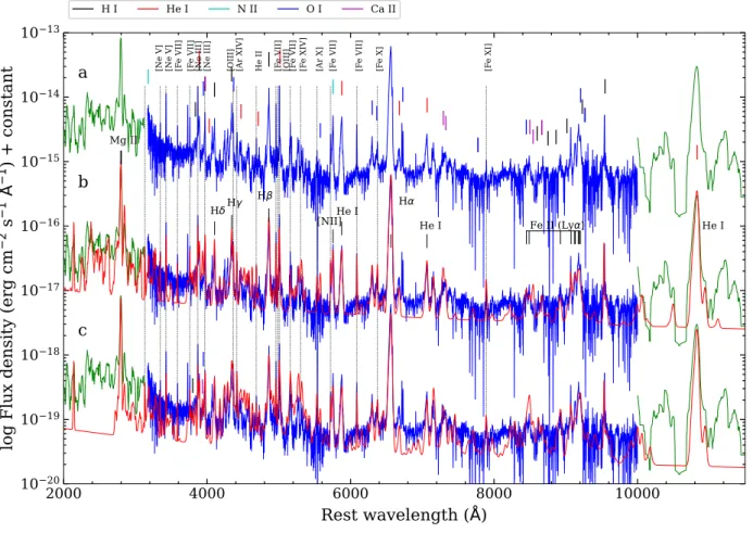
Figure4shows the result of a “best-fit" calculation for the two Fe II line cases mentioned above. For both models, we note a steep Balmer decrement, withF(Hα)/F(Hβ) ≈9. This ratio is compara- ble to that of other SNe IIn (Fransson et al. 2014) and is mainly a result of the large optical depth of Hα. This situation, often referred to as “Case C," is discussed in detail byXu et al.(1992). For the higher-order Balmer lines, as well as the Paschen lines in the NIR, there is good agreement with the observations for this model. Sim- ilar agreement is found for the He I lines, where the comparatively highλ7065/λ5876 ratio, as well as theλ10930/λ5876 ratio, are a result of high optical depth in these lines (seeKaramehmetoglu et al. 2019).

The Fe II emission shows a prominent line feature in the∼ 8450–9200 Å range, with the three peaks at 9076, 9126, and 9177 Å, which are well reproduced by both models. The lines at 8451 Å and 8490 Å also agree well with the simulations, confirming the contribution of Lyαfluorescence. The feature at∼2845 Å is most likely to be Fe II rather than Mg Iλλ2852, 2857. This line complex consists of a number of strong lines from an upperd⁴Dlevel fed by transitions from thev⁴Flevel, which also gives rise to the∼9175 Å peak. The simulations also show the very large number of Fe II lines in the region 4000–6000 Å, which makes an unambiguous identification of other weak lines challenging.

TheSigut & Pradhan(2003) model yields intensities that agree well at most wavelengths, although the∼2848 Å peak is overpro- duced by a factor of∼ 3. The ηCarinae spectrum gives better agreement with the optical range 4000–5500 Å, while the AGN simulation agrees better with the fluorescence features in the NIR and UV. The relative line intensities depend on both the atomic data, especially collisional, and the physical conditions. The AGN environment, for example, has a density of∼4×10⁹cm⁻³, which is much higher than that of the SN CSM. The calculated intensities also depend on the continuum level, which can be quite uncertain.

Regardless of model, however, we find that there is strong evi- dence for the importance of Lyαfluorescence in the spectrum of SN 2005ip.

3.2.2 High-ionisation CSM lines

High-ionisation ions were observed early (Smith et al. 2009b) and grew stronger with time (Smith et al. 2017). Figure4shows that in our most recent spectra, we identify a large number of these high- ionisation lines, including He IIλ4685.6, [O III]λλ4363.2, 4958.9,

2000 4000 6000 8000 10000

Rest wavelength (

)

10

10

10

10

10

10

10

10

log Flux density (erg cm

s

)+ constant

[OIII] [OIII][FeVII] [FeVII] [FeXIV] [ArX] [FeVII] [FeVII] [FeX] [FeXI]

Hα

H^β H^γ H^δ

He I He I [NII] He I Mg II

Fe II (Ly^α)

a

b

c

H I He I N II O I Ca II

Figure 4.Synthetic spectra with line identifications for the UV to MIR spectrum of SN 2005ip at 3065–3165 d. The upper spectrum, (a), shows the observed data (green = near-UV and NIR, blue = optical) with colour-coded line identifications given in the legend above the figure, plus a number of marked high-ionisation lines, described in the text. The middle spectrum, (b), shows the same observed data together with the synthetic spectrum (red). The Fe II spectrum used is taken from the calculations bySigut & Pradhan(2003). Spectrum (c) is the same, but with the the observed Fe II spectrum ofηCarinae fromZethson et al.

(2012). Note especially the strong NIR Fe II lines at∼8450–9200 Å, powered by fluorescence from Lyα.

5006.8, [Ne III] λλ3869.1, 3967.5, [Ne V] λλ3345.8, 3425.5, [Fe VII]λλ3586.3, 3758.9, 4942.5, 4988.6, 5158.4, 5720.7, 6087.0, [Fe X]λ6374.5, and [Fe XI]λ7891.8. In addition, [Ar X]λ5533, [Ar XIV]λ4412.3, and [Fe XIV]λ5302.9 may be present, although likely blended with [Fe II] lines at later epochs.

The numerous [Fe VII] lines offer a diagnostic of the density and temperature from the region where these arise. The FWHM of these lines is∼350 km s⁻¹, similar to the other high-ionisation lines. The main uncertainty of the line fluxes comes from blend- ing and the continuum level. The continuum uncertainty affects the λλ4988.6, 5158.4 lines most. The [Fe VII]λ6087.0 line is an im- portant diagnostic, but nearly coincides with theλ6086.37 line of [Ca V]. From their transition rates, [Ca V]λ6086.37 should have an intensity∼0.19 of [Ca V]λ5309.1. The latter is a blend, but using its peak intensity as an upper limit to the flux and a ratio of theλ6086/λ5309 features of∼2.4, we predict a maximum contri- bution from [Ca V] to theλ6086 line of 8%. We therefore conclude that this line is mainly due to [Fe VII]. The [Fe VII]λλ3586.3, 3758.9 lines have a common upper level and their ratio is therefore fixed by their transition probabilities to 1 : 1.5, which agrees with the observed ratio, and we therefore only discuss theλλ3586.3 line.

From the observed spectrum at 905 d,F(λ3586)/F(λ6087) ≈ 1.08 andF(λ5721)/F(λ6087) ≈0.57. At 3399,d the corresponding ratios areF(λ3586)/F(λ6087) ≈0.84 andF(λ5721)/F(λ6087) ≈ 0.61. The uncertainties in these ratios mainly come from the as- sumed reddening and the continuum level, and we estimate these to be∼30%. Because of blending, the other ratios have considerably larger estimated uncertainties.

Figure5plots the theoretical line ratios for the strongest lines as a function of the electron density for temperatures from 10⁴K to 10⁵K. Collision strengths are obtained fromBerrington et al.(2000) and transition rates are obtained from NIST with a 9-level model atom. All ratios are relative to the strongλ6087.0 line. Overplotted are the measured line ratios from days 905 and 3099.

We place the most emphasis on the strongest lines, represented by theF(λ3586)/F(λ6087) and F(λ5721)/F(λ6087) ratios. The strong temperature dependence of theF(λ3586)/F(λ6087)ratio, together with theF(λ5721)/F(λ6087)ratio, points to a temperature

&3×10⁴K on day 905 and&2×10⁴K on day 3099. Day 905 may

have a temperature as high as∼10⁵K. Photoionisation calculations for X-ray-illuminated plasmas byKallman & McCray(1982) (e.g., their Model 3) show that Fe VII is most abundant at∼3×10⁴K, 000

10

10⁴ 10⁵ 10⁶ 10⁷ 10⁸ 10⁹ 10¹⁰

electron density (cm

)

10 ¹ 10⁰ 10¹

lo g F/ F( 60 87 ) 905 d 905 d 905 d 905 d 905 d 5720 5159 4989 4942 3586

10⁴ 10⁵ 10⁶ 10⁷ 10⁸ 10⁹ 10¹⁰

electron density (cm

)

10¹ 10⁰ 10¹

lo g F/ F( 60 87 ) 3099 d 3099 d 3099 d 3099 d 3099 d 5720 5159 4989 4942 3586

Figure 5.Line ratios of the optical [Fe VII] lines relative to theλ6086 line as a function of density for 10,000 K (solid lines), 20,000 K (dot-dashed lines), 30,000 K (dashed), and 100,000 K (dotted). The left panel shows the observed ratios at 905 d while the right is the same for 3099 d. The vertical dashed lines shows the density range compatible with the different line ratios. The colour code of the modelled and observed ratios is given in the legend. The solid horizontal lines give the observed ratios, while the dashed lines indicate approximate error bars.

consistent with these observations. For comparison, Fe XIV, which is seen in at least the earlier spectra, arises at∼6×10⁴K.

The electron density is∼4×10⁶–3×10⁷cm⁻³for day 905, and a similar density range,∼4×10⁶–2×10⁷cm⁻³, for day 3099. It is difficult to draw any strong conclusions about a changing density between these epochs, but a decrease should have been expected. As pointed out byBerrington et al.(2000), there is likely considerable uncertainty in the atomic data, adding to the uncertainty in the ob- served fluxes. However, even considering this, it is quite remarkable that the SN is interacting with a CSM with density&4×10⁶cm⁻³

at&3000 d after explosion.

The density we find here can be compared to the density in- ferred from the bolometric light curve in Sec.3.1. With a mass-loss rate MÛ ≈ 1×10⁻²⁻¹Myr⁻¹ and velocity∼ 3000 km s⁻¹ at

∼ 1000 d, one obtains a density∼ 4.5×10⁶⁻¹cm⁻³ at 1000 d.

While this is compatible with the range we find above from the for- bidden lines, one should note that the density from the bolometric light curve depends onand is therefore only a lower limit; it may be up to an order of magnitude higher. We also note that the forbid- den lines are not affected by electron scattering and should therefore arise in a region different from that responsible for the bulk of the radiation, close to the shock. A natural scenario is therefore that the forbidden, high-ionisation lines arise outside the region close to the shock which is optically thick to electron scattering, and where the Balmer lines and most of the radiation originate.

3.2.3 The UV spectrum

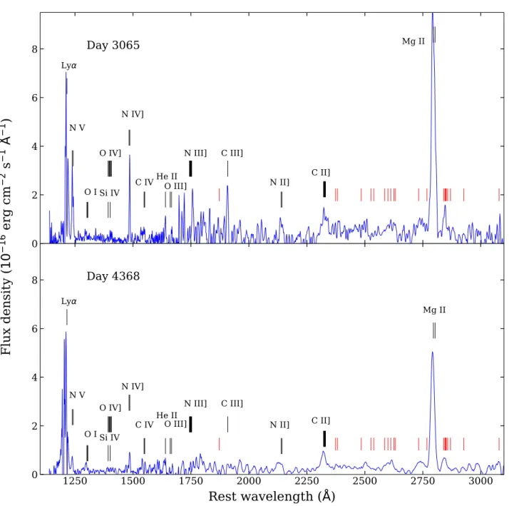
Figure6shows the extracted UV spectra (no background subtrac- tion is applied) and identifies the UV spectral lines, including the strong presence of Lyα, N v λλ1238.8, 1242.8, N iv λλ1483.3, 1486.5, N iii]λλ1746.8–1754.0, C iii]λλ1906.7, 1908.7, and Mg ii λλ2795.5, 2802.7. Weaker lines also exist, specifically He iiλ1640, N II]λλ2139.0, 2142.8, and C ii]λλ2323.5–2328.1. We identify the feature at∼2600 Å with the Fe II 4sa⁶Dto 4pz⁶D⁰multiplet.

Table 8.Reddening-corrected fluxes of strong UV lines from day 3065.

Species Wavelength Flux Uncertainty (Å) (10⁻¹⁵erg s⁻¹cm⁻²)

N v 1238.8, 1242.8 4.80 0.07

N iv] 1483.3, 1486.5 2.72 0.15 C iv 1548.2, 1550.7 1.14 0.11

He ii 1640.4 0.88 0.26

O iii] 1660.8, 1666.2 <0.5 – N iii] 1746.8–1754.0 3.01 0.35 C iii] 1906.7, 1908.7 2.55 0.34

There may be additional blends at∼ 2500 Å and∼ 2750 Å, but their signal-to-noise ratio (S/N) is lower. We note that the N iii]

λλ1746.8–1754.0 multiplet is redshifted to∼1758 Å.

Table8lists the reddening-corrected fluxes for the strongest UV lines from day 3065 shown in Figure6(with the background level subtracted). Several caveats should be noted. The low S/N in the region above 1700 Å makes the continuum difficult to esti- mate, so the systematic error is approximated by comparing different wavelength ranges from the lines. The flux of C ivλλ1548, 1551 is likely underestimated owing to the presence of both the Galactic and host-galaxy ISM absorption. The O iii]λ1664 line is weak and in a noisy region of the spectrum, so the calculated flux should only be considered an upper limit.

An estimate of the CSM density for the first epoch can be ob- tained from the ratio of the N iv]λ1483.3 andλ1486.5 lines, which we calculate to beλ1483.3/λ1486.5≈0.3. For an X-ray-ionised plasma the N IV abundance peaks where the temperature is (2–3)

×10⁴K (Kallman & McCray 1982). Most important, the line ratio is sensitive to density but relatively insensitive to temperature. From Figure 1 ofKeenan et al.(1995), the observedλ1483.3/λ1486.5 ratio corresponds to an electron density of (2.0–3.6)×10⁵cm⁻³in the temperature range (1–2)×10⁴K. We conclude that the CSM

0 2 4 6

8 Ly

N V

O I Si IV O IV]

N IV]

C IV He II O III]

N III] C III]

N II] C II]

Mg II

Day 3065

1250 1500 1750 2000 2250 2500 2750 3000

Rest wavelength ( ^Å )

0 2 4 6 8

Ly

N V O I Si IV

O IV]

N IV]

C IV He II O III]

N III] C III]

N II] C II]

Mg II

Day 4368

Flux density ( 10

erg cm

s

Å

)

Figure 6.HST/STIS spectra of SN 2005ip on days 3065 and 4368 post-explosion. No extinction correction or background subtraction is applied. The wavelengths of probable line identifications are shown. The red vertical bars mark the wavelengths of the strongest Fe II lines from the list ofSigut & Pradhan(2003).

density should be safely lower than the critical densities of the semiforbidden lines.

3.2.4 Line profiles

Figure7compares the velocity profile of several UV and optical lines at∼3100 days. The Hαline extends to∼2600 km s⁻¹on the blue side and only∼1000 km s⁻¹on the red. Hβ, He iλ5876, and Mg iiλλ2796, 2803 have similar line profiles. While the blue side can be well fit with an electron-scattering wing, the line centroid is shifted to the blue, with a “shoulder" at ∼ −800 km s⁻¹. As shown byTaddia et al.(2020) andDessart et al.(2015), this type of profile can be explained by a combination of emission from the shock wave and emission from the pre-shock CSM. The emission

from the shock is responsible for the blueshifted shoulder, while the central component is coming from pre-ionised gas in the CSM. Both components are affected by electron scattering in the low-velocity CSM. This gives rise to the smooth, blue wing shortward of the

“shoulder." Because of the smoothing by the electron scattering, the velocity of the “shoulder" is lower than the shock velocity.

Both Hβand He I λ5876 have line profiles similar to that of Hα, as expected if these arise from similar regions (Fig.7). The Lyαline has a profile broadly consistent with Hα, although strongly distorted by a central absorption feature from both the Galactic and host-galaxy ISM.

The C iii], N iii], N iv], and N v UV lines are considerably narrower than Hα, and consistent with being unresolved at the∼ 300 km s⁻¹instrumental resolution of STIS. These lines do not show the velocity shift of the Balmer and He I lines, and most likely come 000