Table S1. Mean Ellenberg indicator values for each site (L: light; N: nutrients; R: soil pH; T: temperature; U: moisture).
Bedrock Management Age year
Average Ellenberg
value L
Average Ellenberg
value N
Average Ellenberg
value R
Average Ellenberg
value T
Average Ellenberg
value U
Limestone active coppice 5 6.49 4.76 6.70 5.97 4.30
Sandstone active coppice 9 5.89 5.40 6.65 5.71 4.76
Sandstone active coppice 14 5.02 4.82 6.20 5.60 4.76
Limestone active coppice 14 5.19 4.80 5.89 5.57 4.60
Sandstone active coppice 25 5.03 5.06 7.97 5.23 4.73
Limestone abandoned coppice 30 4.45 6.03 6.56 5.49 4.98
Sandstone abandoned coppice 49 4.42 5.21 7.09 5.41 4.91
Sandstone abandoned coppice 56 4.09 5.54 6.20 4.82 5.06
Limestone old growth unmanaged >400 (190) 4.63 5.63 6.67 5.00 4.89 Limestone old growth unmanaged >400 (190) 4.10 6.10 6.67 4.86 4.90 Limestone old growth unmanaged >400 (190) 4.53 6.29 8.38 5.07 4.76
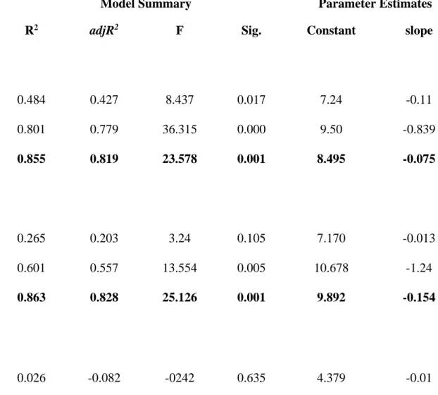
Table S2. Parameters of the three best performing regression models describing changes of Compositional Diversity and Bray-Curtis Dissimilarity percentage for all species and specialist species at two different spatial scales. We selected the model explaining the highest variance (R2) marked in bold.
Model Summary Parameter Estimates
Dependent variable/Models R2 adjR2 F Sig. Constant slope
Compositional Diversity ALL species - 10 m
Linear 0.484 0.427 8.437 0.017 7.24 -0.11
Logarithmic 0.801 0.779 36.315 0.000 9.50 -0.839
Quadratic 0.855 0.819 23.578 0.001 8.495 -0.075
Compositional Diversity ALL species - 2 m
Linear 0.265 0.203 3.24 0.105 7.170 -0.013
Logarithmic 0.601 0.557 13.554 0.005 10.678 -1.24
Quadratic 0.863 0.828 25.126 0.001 9.892 -0.154
Compositional Diversity Specialist species - 10 m
Linear 0.026 -0.082 -0242 0.635 4.379 -0.01
Logarithmic 0.022 -0.086 0.205 0.661 4.559 -0.077
Quadratic 0.031 -0.201 0.132 0.878 4.293 -0.003
Compositional Diversity Specialist species - 2 m
Linear 0.049 -0.057 0.464 0.513 3.444 0.002
Logarithmic 0.000 -0.111 0.000 0.983 3.628 -0.005
Quadratic 0.336 0.170 2.023 0.195 4.219 -0.038
Bray-Curtis Dissimilarity ALL species - 10 m
Linear 0.079 -0.23 0.775 0.402 68.481 -0.044
Logarithmic 0.007 -0.103 0.63 0.808 68.248 -0.800
Quadratic 0.722 0.524 12.345 0.03 50.780 -0.043
Bray-Curtis Dissimilarity ALL species - 2 m
Linear 0.151 0.056 1.59 0.238 79.237 -0.037
Logarithmic 0.045 -0.060 0.433 0.527 81.133 -1.258
Quadratic 0.356 0.195 2.209 0.172 73.407 0.264
Bray-Curtis Dissimilarity Specialist species - 10 m
Linear 0.047 -0.059 0.440 0.524 64.540 -0.042
Logarithmic 0.001 -0.110 0.006 0.941 62.701 -0.301
Quadratic 0.625 0.337 13.245 0.021 43.992 -0.005
Bray-Curtis Dissimilarity Specialist species - 2 m
Linear 0.000 -0.111 0.000 0.988 69.465 0.001
Logarithmic 0.019 -0.090 0.174 0.686 65.688 1.068
Quadratic 0.182 -0.022 0.891 0.447 62.216 -0.002
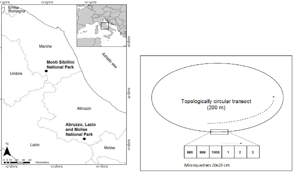
Figure S1. Location of the study areas in the context of central Italian Apennines (on the left, thanks to Flavio Marzialetti)and scheme of the topologically circular transect used to sample understory vegetation (on the right).
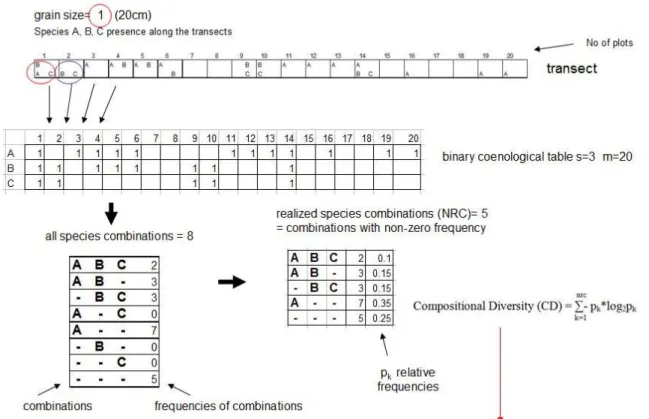
Figure S2. Illustration of computerized sampling and the calculation of Compositional Diversity using artificial data. 1, The baseline transect (20 units long with 3 species) resampled with computer (with grain size =1) and a binary coenological table is created. 1, Species combinations counted from the binary coenological table. 3, Number of realized species combinations (NRC) are the number of combinations with non-zero frequency (from 3 species the potential maximum number of combinations would be 8, however, only 5 had non-zero frequency in our example (NRC=5). 4, Compositional Diversity, i.e. the diversity of species combinations is calculated based on the relative frequency of species
combinations.
Figure S2a. Example for calculating Compositional diversity with grain size=1
Figure S2b. Example for calculating Compositional diversity with grain size=2
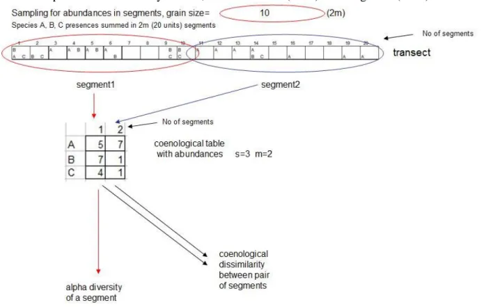
Figure S2c. . Illustration of computerized sampling from the base-line transect for calculating traditional alpha and beta diversity indices. 1, After selecting a specific scale (2m in our example, i.e. grain size = 10) the transect was subdivided into 2m segments and 2, abundances of species were determined by summarizing presences of species within each segment (at 2 m scale abundance scores range from 0-10). 3, Coenological table was formed from abundance data. 4, Alpha diversity was calculated for each segment and coenological dissimilarity was calculated for each pair of segments. 5, Mean of these indices was used to characterize the whole community. 6, As an alternative representation of beta diversity, spatial CV% of alpha diversity estimates (i.e. CV% of segment-scale estimates) was also created. See main text for the name of particular alpha and beta diversity indices, and see Podani (2000) and Magurran (2004) for the related formula.
References
Podani, J. Introduction to the Exploration of Multivariate Biological Data Backhuys Publishers, Leiden, The Netherlands. 2000, 407. p.
Magurran, A. Measuring Biological Diversity; Blackwell Science Ltd.: Oxford, UK, 2004, 256. p.
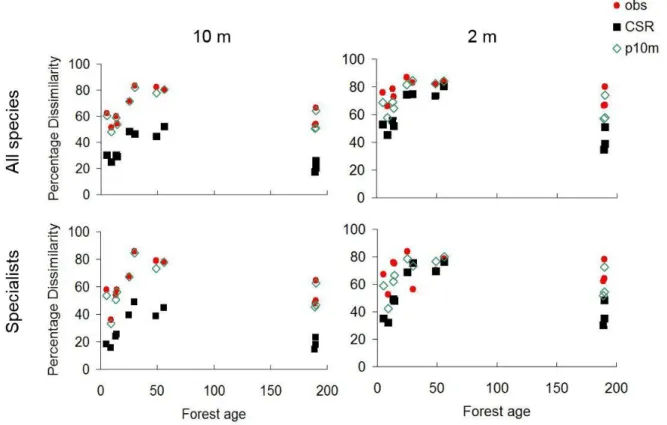
Figure S3. Beta diversity trends along the chronosequence (represented by Bray-Curtis Dissimilarity). obs = Observed data, CSR = null model based on Complete Spatial Randomizations, p10m = Patch model randomization with 10m diameter.
Figure S4. Example of spatial patterns detected in the field. Points represent presences in 20 x 20 cm contigous sampling units along the sampled transects (for better resolution only 100m subsets are shown) . Species belonging to the same Social Behaviour Types (SBT1=beech forest
specialists, SBT2= forest generalists, others (forest edge-, open habitat- and weedy species) were merged here (for demonstrative purposes).
For more details about Social Behaviour Types cf. Bartha et al. 2008. [5].