Optimization of peak capacity

Contents

1 Optimization of peak capacity 3

1.1 Introduction . . . 3

1.2 Theory . . . 5

1.2.1 Peak capacity in isocratic elution . . . 7

1.2.2 Peak capacity in gradient elution . . . 9

1.3 Optimization of peak capacity . . . 11

1.3.1 Optimization of isocratic separations . . . 12

1.3.2 Optimization of gradient separations . . . 23

1.4 Conclusions . . . 30

References . . . 35

Chapter 1

Optimization of peak capacity

1.1 Introduction

The ultimate goal of analytical liquid chromatography is to provide high separation power in the shortest time possible. In HPLC, performance means peak width. The higher the perfor- mance of a chromatographic method, the narrower the peaks are on the chromatogram. Several measures exist for the quantification of quality of a separation or of a chromatogram. The most commonly used one is the number of theoretical plates, N, which is considered as a bench- mark measure. The use of plate count, however, has disadvantages. Although it can estimate widths of peaks in isocratic measurements, it cannot be used in gradient separations directly, nor it can tell anything about the overall separation power of the chromatographic method. A column even with the highest plate count ever is useless if all the compounds elute together in a very narrow time range. Resolution, on the other hand, can be used for the characterization of separation quality of neighboring compounds in both isocratic and gradient runs. However, resolution does not serve any information on the general column performance. Peak capacity, a concept introduced by Giddings [1] in 1967, is a very intuitive and at the same time much more general measure than plate count and resolution. Peak capacity is the maximum number of components resolvable by HPLC with a unity resolution [2]. It combines the entire chromato- graphic space with the variability of the peak widths over the chromatogram. While the number of the actually resolved peaks depends on the nature of solutes existing in a particular mixture, peak capacity can be used to approximate the overall separation power of a given column. Since the introduction of the peak capacity concept, it has been used widely in chromatography both in theoretical studies and method developments.

In method development, peak capacity has a significant importance in analysis of complex samples (e.g. protein tryptic digests). Complete resolution of all components in these samples is often impossible by unidimensional chromatography due to the large number of compounds, even if it is smaller than the peak capacity offered by the method. In that case, the analyst should

focus on decreasing the degree of overlap of the components by maximizing the peak capacity of the system. When simpler mixtures containing much fewer components are analyzed, the optimization of resolutions of pairs of compounds by adjusting the selectivities through the variation of separation conditions is a suitable approach. The effectiveness of this concept, however, is limited as the number of components becomes much larger than 15–20 [3].

Comparison of separations is not always a straightforward task. Giddings introduced [4]

the concept of kinetic plots to compare the theoretical limit of separating speed of gas and liq- uid chromatography by plotting the logarithm of analysis time against the logarithm of plate count. This approach was used and extended by Knox and Saleem [5], and Guiochon [6]. In 1997, Poppe [7] proposed to plot plate time, t₀/N, against N to obtain a clearer comparison of chromatographic columns. Desmet et al. [8] extended Gidding’s concept and generated a broad family of kinetic plots which allow the direct comparison of the performance of different LC supports. Since its introduction, applications of Poppe plots become widespread in devel- opment and evaluation of stationary phases and efficient chromatographic methods. Even if Poppe plots were constructed for isocratic separations originally, they were extended for gra- dient [9] chromatography as well. In these approaches the gradient times are used instead oft₀ to generate the Poppe plots.

In this chapter, possible concepts are presented for the optimization of chromatographic peak capacities. The majority of the results are dedicated to reversed-phase gradient chro- matography, or at least separations modes where the linear solvent strength model [10] applies.

The most important algorithms used for the calculation of results of this chapter are pre- sented in Python programming language¹. The reader can use, modify and share it freely without the permission of the author. The main reasons of using Python in optimization of chromatographic separations are the following:

• Python is free and open source, whereas other closed-source commercial products can sometimes be very expensive,

• Python is easy to read and has relatively short learning curve,

• Python integrates well with other languages (e.g. C/C++, Fortran),

• a large number of general-purpose or more specialized libraries exists for Python,

• a huge scientific community is built up around Python. It is easy to find help and infor- mation from other scientists.

1https://www.python.org/

this chapter based on NumPy² and SciPy³ libraries. These two libraries together cover most of MATLAB’s basic functionality and parts of many of the toolkits. Additionally, they have great documentation and an active community. The figures were generated with the Matplotlib⁴ plotting library which is able to produce publication quality figures in a variety of formats and interactive environments.

As of the writing of this chapter (autumn of 2017), Python 3.6, NumPy 1.13, SciPy 1.0, and Matplotlib 2.0 are the actual versions of the language and libraries. The codes shared in this chapter were tested and worked with these versions. Even if Python language and its libraries are evolving gradually, the codes can be used directly or with slight modification at least a decade after publishing this book most probably. Note that Python uses indentation to structure its programs and scripts into blocks. When using the codes presented in Listings 1.1 –1.6, please pay careful attention to the leading spaces at the beginning of lines.

The author of this chapter recommends the installation of a Python distribution. In 2017, the two most popular and complete distributions aimed at the need of scientific community are Anaconda Python Distribution⁵ and Enthought Python Distribution⁶. These distributions contains all the necessary tools and libraries required to run the Python codes presented in Listings 1.1–1.6.

A part of the Python codes used during the construction of figures presented in this Chapter were common in each program. In Listing 1.1, imports of the libraries, definitions of func- tions and constants that are necessary to run all the other codes are presented. The content of Listing 1.1 should be copied before the codes presented in Listings 1.2 –1.6.

1.2 Theory

Peak capacity is the measure of the number of peaks that can fit into an elution time window t₁ tot_n with a fixed — usually unity — resolution [2]. There are several approaches for the derivation of peak capacity. Originally, it was defined by Giddings for isocratic chromatography [1] and subsequently extended by Horváth and Lipsky [11] to gradient elution chromatography.

Grushka [12] later also derived an equation for computing peak capacity in gradient elution.

Here, we follow Grushka’s approach that is general enough to apply for both isocratic and gradient separations as well. According to this approach, peak capacity of a chromatographic separation can be calculated by the solution of an ordinary differential equation.

2http://www.numpy.org/

3https://www.scipy.org/

4http://matplotlib.org/

5http://www.anaconda.com/distribution/

6http://www.enthought.com/product/enthought-python-distribution

import matplotlib.pyplot as plt #import of Matplotlib library import numpy as np #import of NumPy library

#import functions from SciPy library

from scipy.optimize import brentq, minimize, curve_fit

def trgrad(tg, fi0, dfi, t0, S, k0):

"""

Calculation of gradient retention time.

For meaning of parameters, see Eqs. (1.12)-(1.21)

"""

b = S*dfi/tg*t0

kfi0 = k0*np.exp(-S*fi0)

return t0*(1 + np.log(1+kfi0*b)/b) def peakcap(tg, fi0, dfi, t0, H, L, S, k0):

"""

Calculation of gradient peak capacity.

For meaning of parameters, see Eqs. (1.12)-(1.21)

"""

N = L/H

b = S*dfi/tg*t0

kfi0 = k0*np.exp(-S*fi0) kL = kfi0/(1+kfi0*b) p = b*kfi0/(1+kfi0)

Theta = np.sqrt((1+p+1/3*p**2))/(1+p) Q = np.sqrt(1 + b + 1/3*b**2)

tau = 1+kfi0*b

return 1 + np.sqrt(N)/4/Q*np.log((b/6 + 1/b*(Q**2*tau-1) + Theta*Q*tau*(1+kL))/(1+b/2+Q)) def peakcapProduction(tg, fi0, t0, H, L, S, k0):

"""

Calculation of gradient peak capacity production, (tG+t₀)/n.

For meaning of parameters, see Eqs. (1.12)-(1.21)

"""

dfi = brentq(lambda dfi: trgrad(tg, fi0, dfi, t0, S, k0)-t0-tg, 1e-6, 1-fi0) return (tg+t0)/peakcap(tg, fi0, dfi, t0, H, L, S, k0)

def h(nu, A, B, C):

"""

Calculation of height equvalent to a theoretical plate.

For meaning of parameters, see Eqs. (1.31) and (1.32)

"""

return A*nu**(1/3)+B/nu+C*nu

A, B, C = 1.0, 1.5, 0.05 #parameters of Knox equation Eq (1.31)

fi = 1e3 #column resistance factor

eta = 1e-3 #dynamic viscosity (Pa sec), dm = 1e-9 #diffusion coefficient, m²/sec

Listing 1.1: Libraries, constants, and function definitions necessary to run Listings 1.3–1.6.

dt =

w(t) (1.1)

with the following initial condition

n(t₁) =1 (1.2)

wherewis peak width generally referred as four times standard deviation of a chromatographic peak (w=4σ),t is time, andt₁the retention time of the first eluting compound.

The solution of Eq. (1.1) requires the knowledge of peak widths as a function of retention time,w(t). The general solution can be written as

n=1+ Z _tn

t₁

1

w(t)dt (1.3)

wheret_nis the retention time of the last peak. Accordingly, the width of accessible separation window ist_n−t₁.

1.2.1 Peak capacity in isocratic elution

Under isocratic elution conditions, the velocity of the sample bands are constant throughout the column. Widths of peaks affected solely by kinetic processes⁷. The dependency of peak widths on retention time can be written as

w(t) = 4

√N t (1.4)

Therefore, solution of Eq. (1.1) is

n=1+

√N 4 lnt_n

t₁ (1.5)

t_ncan be rewritten as the sum oft₁and the relative retention window

t_n=t₁(1+δ) (1.6)

whereδ is the width of retention window relative to the retention time of the first compound δ =t_n−t₁

t₁ (1.7)

Note thatδ is the retention factor,k, whent₁equals to the column hold up time,t₀.

7This statement is strictly true only under linear conditions when the isotherm of compounds are linear. Under non-linear conditions, thermodynamic processes also influence peak shapes.

0 5 10 15 20 25 30 0.0

0.2 0.4 0.6 0.8 1.0

n/ N

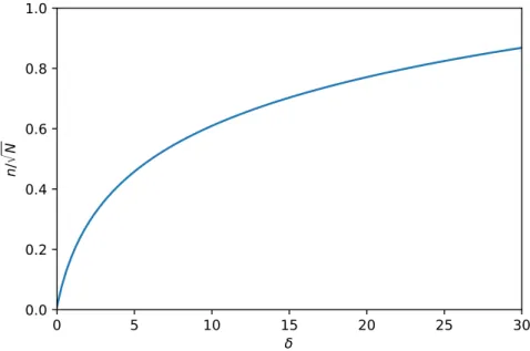
Figure 1.1: Isocratic peak capacity relative to the square root of N as a function of relative retention window,δ.

By combining Eqs. (1.5)–(1.7) peak capaity can be expressed as n=1+

√N

4 ln(1+δ) (1.8)

In Fig. 1.1, the isocratic peak capacity relative to the square root of N can be seen as a function ofδ. The figure shows that the wider the retention window the higher the achievable peak capacity is. The increase ofn, however, is less remarkable at largerδ values.

It is important to note that peak capacity of isocratic separations is not the ratio of the retention window and average peak width. That would be

t_n−t₁

w = t_n−t₁

1 tn−t1

Rtn

t1 w(t)dt =

√N 2

t_n−t₁

t_n+t₁ (1.9)

In the equations above, the extra column band broadening was not taken into account. In several cases, however, extra column processes have a large impact on the width of peaks. As- suming that the extra column variance isσ_ext² , peak widths and peak capacities can be rewritten as

w(t) =4 rt²

N+σ_ext² (1.10)

n=1+

√N 4 ln

1+δ+ r

(1+δ)²+^σext2

σ₁²

1+ r

1+^σext2

σ₁²

(1.11)

whereσ₁²is the variance of the first eluting peak.

1.2.2 Peak capacity in gradient elution

In gradient chromatography, eluent composition is varied during the separation in order to grad- ually decrease the retention of solutes. Estimation of retention times and peak widths requires the solution of two ordinary differential equations [13] and the knowledge of the change of eluent composition as a function of time,ϕ(t)and the relationship between the retention factor and eluent composition, k(ϕ). In gradient chromatography, it is impossible to derive general equations for the estimation of peak capacity due to the wide variety of the parameters that affect peak shapes. Several assumptions has to be defined regarding the shape of gradient and retention behavior of compounds.

Poppe et al. [13] derived simplified equations for the calculation of retention times and peak variances in the case of linear gradients and linear solvent strength (LSS) behavior that means that the composition of stronger eluent component was a linear function of time, and that the isocratic retention of a solute (lnk) was assumed to be a linear function of the volume fraction of the stronger eluent modifier (ϕ):

k=k₀exp(−Sϕ) (1.12)

wherek₀ the retention factor of the compounds forϕ = 0,−S the slope of lnk[ϕ]vs. ϕ plot.

Sis a practical measure of the retention sensitivity of a compound toward the change of eluent composition.

Under these conditions, the retention time of a compound,t_R, and the width of its peak can be calculated by the following set of equations [13]:

t_R=t₀ 1+ln k_ϕ0b+1 b

!

(1.13)

w=4 L

√N 1+k_L

u₀ Θ (1.14)

withbthe gradient steepness

b=S t₀∆ϕ

t_G (1.15)

where∆ϕis the change of stronger eluent component int_Ggradient time,k_Lthe retention factor of the compound at the column outlet. Θ represents the band compression [14, 15] that arises from the rear part of the band migrating at a velocity higher than the front part.

k_L = k_ϕ0

1+k_ϕ0b (1.16)

and

Θ = q

1+p+¹₃p²

1+p (1.17)

where

p=b k_ϕ0

1+k_ϕ0 (1.18)

andk_ϕ0 is the retention factor of solute at the beginning of analysis (ϕ =ϕ₀)

By rearranging Eq. (1.13) fork_ϕ0 and substituting it into Eq. (1.14) ,w(t)can be generated.

It still cannot be integrated since the value ofbis different from solute to solute. Accordingly, an additional assumption has to be made regarding the constant values ofSfor all the sample compounds. In that case, peak capacity of linear gradients in case of LSS behavior becomes

n=1+

√N 4

1 Qln

b

6+¹_b Q²τ_n−1

+Θ_nQτ_n(1+k_L,n) 1+^b₂+Q

!

(1.19) with

Q= r

1+b+1

3b² (1.20)

and

τn=exp

b t_n

t₀−1

(1.21) wherek_L,nandΘn refers to the last eluting compounds [see Eqs. (1.16) and (1.17)]. Note that Eqs. (1.19)–(1.21) are essentially the same as Eqs. (14)–(17) of Ref. [16] derived by Gritti and Guiochon. However, here they are presented in a different grouping of parameters.

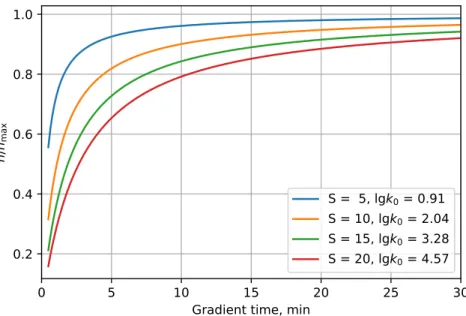
In Fig. 1.2, gradient peak capacities as a function oft_Gcan be seen at different combination of S and k₀ parameters. As opposed to isocratic separations (see Fig 1.1), peak capacities approach a maximal peak capacity as analysis time increases in gradient separations. The maximal peak capacity that can be achieved with gradient elution can be determined as the limit of Eq. (1.19) ast_Gapproaches infinity.

n_max=1+

√N

4 ln 1+k_ϕ0,n

(1.22) wherek_ϕ0,nis the retention factor of the last eluting compound at the beginning of analysis.

Peak widths and peak capacities calculated by Eqs. (1.14) and (1.19) are valid in ideal case.

0 5 10 15 20 25 30 Gradient time, min

0.2 0.4 0.6 0.8 1.0

n/ n

S = 5, lgk

= 0.91 S = 10, lgk

= 2.04 S = 15, lgk

= 3.28 S = 20, lgk

= 4.57

Figure 1.2: Gradient peak capacity relative to n_max as a function of gradient time, t_G. Pa- rameters of calculation: column length L=10 cm, particle diameterd_p=1.7µm, pressure drop

∆P=1200 bar, plate countN=25 000, column hold-up timet₀=28.8 sec.

In practice, several effects cause peak broadening downstream the column (e.g., peak spreading in tubings, connections, detector cell, etc.). Since the retention factor of compounds are large at the beginning of analysis, solutes are focused in narrow bands at the head of column after injec- tion. Therefore, the pre-column effects usually do not affect final peak shapes. Thus, the peak variance has to be completed with the contributions of post column broadening. Accordingly, widths of detected peaks can be calculated as:

w'4 s

L² N

1+k_L u₀

2

Θ²+σ_t,pc² (1.23)

whereσ_t,pc² represents the contribution of the post-column processes to the variance of the peak.

1.3 Optimization of peak capacity

In practice, optimization of peak capacities are necessary when the sample contains large num- ber of compounds. In that case the goal usually is not the complete baseline separation of all compounds, but the spreading of analytes as much as possible before introduction into mass spectrometer or a second chromatographic dimension. The analyst usually has two different goals: (1) achieving a given target peak capacity within as short time as possible, or (2) reach- ing the highest possible peak capacity in a given analysis time. In the following general con-

cepts and considerations are presented that are applicable to fulfill both goals of peak capacity optimization.

1.3.1 Optimization of isocratic separations

Close examination of Eq. (1.11) highlights that peak capacity in isocratic mode can be opti- mized by:

• minimizing the extra-column band broadening (σ_ext² ),

• maximizing the retention window (δ), and

• maximizing column efficiency (N).

Extra-column band broadening

It is well known that extra column band broadening has a deteriorating effect on separation performance. The relative decrease of apparent column plate count depends on the relation of column- and extra-column variances.

∆N

N =− σ_ext² σ_col² +σ_ext²

=− σ_ext²

t_R² N+σ_ext²

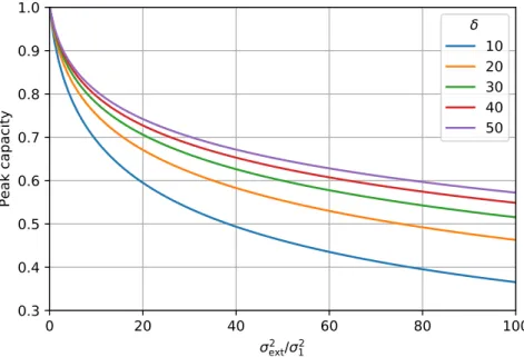
(1.24) Typical values of contributions of UHPLC, optimized HPLC, and non-optimized HPLC systems to the peak variances are 5, 25, and 100µL² [17, 18], respectively⁸. Note, however, that the actual values vary from instrument to instrument. Since column variance is proportional to the square of retention time, the deteriorating effect of extra-column band broadening is more significant for the early eluting compounds. In Fig. 1.3, the decrease of peak capacities can be seen asσ_ext² /σ₁²ratio varies. The volumetric variance of a peak eluted at the hold-up time from a 150×4.6 mm column packed with 5µm particles is typically larger than 175µL². Therefore, σ_ext² /σ₁² is lower than 0.5 when an older HPLC instrument is used. Less than 5% decrease of peak capacity should be expected in that case. Using a 50×2.1 mm column packed with 1.7µm particles, however, the variance of the peak eluting with the column dead volume can be less than 1µL². Even a state of the art instrument with a 5µL² extra column variance can decrease the peak capacity with more than 10%. Using these columns in outdated, non- optimized instrument, the peak capacity might be lower than half of that provided by the column itself. The effect ofσ_ext² is more significant when the retention window is narrow. Note, that

8Because of practical reasons, volumetric variances are usually used for the quantification of extra column band broadening (see Refs. [17, 18]). By dividing it with the square of flow rate, volumetric variances can be converted to temporal variances. Similarly, temporal variances can be converted to volumetric ones by multiplying with the square of flow rate. Therefore, volumetric variance of a chromatographic peak is the ratio of square of retention volume to the plate number,V_R²/N.

0 20 40 60 80 100

2ext

/

0.3

0.4 0.5 0.6 0.7 0.8 0.9 1.0

Peak capacity

10 20 30 40 50

Figure 1.3: Relative peak capacity as a function of ratio of extra-column and column variance at different width of retention windowδ.

the decrease of peak capacity is unaffected by the actual column plate number in practice when N is sufficiently large.

It can be concluded that extra-column processes might have significant effect on the achiev- able peak capacity depending on the type of column and instrument used. Accordingly, the extra column effects cannot be neglected in the optimization of isocratic peak capacities, espe- cially when ultra-high performance columns are used. The minimization ofσ_ext² by reducing volumes of capillaries and detector is necessary when the goal of separation is to achieve high peak capacities in a reasonable analysis time.

Width of retention window

Eq. (1.11) clearly shows that the wider the retention window the more powerful the separation is. After some simple considerations, the relative retention window,δ, can be rewritten as

δ =







(α−1)_1+k^k1

1 ifk₁>0 k_n ifk₁=0

(1.25)

whereα is the selectivity of the last and first eluting solutes,α =k_n/k₁.

Eq. (1.25) has similar form than the simplified resolution equation that is one of the most important relationships in development and optimization of isocratic separations (see e.g.

Eq. (2.24) of Ref. [19]). Eq. (1.25) serves with the important conclusion that peak capacity

of isocratic separations can be improved by the increase ofα.

The selectivity between the first and last eluting solutes can be adjusted by the proper choice of stationary phase and separation conditions. Variation of mobile phase composition can be a suitable strategy if the compounds respond differently to the change of eluent composition. In reversed phase and hydrophilic interaction modes this condition applies usually. Especially in the case of analysis of biological samples. In ion chromatography, however, only selectivities of ions having different charge can be modified by the change of the concentration of electrolyte.

When the ions have the same charge, other approaches should be applied for the variation ofα (e.g. addition of organic modifier to the eluent).

The change of separation temperature can also be a suitable option for the selectivity im- provement. Especially, when the difference between the adsorption enthalpies,∆H, of the first and last eluting compounds are large. Since late eluting solutes usually have higher affinities toward the stationary phase, the decrease of temperature might improveα. Note, however, that it increases the pressure drop of the column and might decreases the overall column efficiency significantly.

Eq. (1.25) shows that by increasing the retention factor of the first eluting peak, k₁, peak capacity of isocratic separation can also be improved supposing thatα remains constant. Note, however, that this scenario is rather theoretical, it does not have any significance in practice.

Increasing the retention of the first eluting compound whileα is kept constant would increase the analysis time so drastically that the cost of analysis in time and solvent consumption would be too much for the extra information gained by the improved peak capacity. Instead, during the optimization of isocratic separations,α should be maximized by increasingk_nand decreasing k₁as low as possible, ideally until zero.

It is worth studying the rate of peak capacity production,νn, with the increase of analysis time. Rate of peak capacity production can be defined as

ν_n= dn dt_n = 1

4

√N

t_n (1.26)

Eq. (1.26) reveals that νn is the highest at the beginning of chromatogram (tn=t₀) and it decreases gradually as the time passes. The rate of peak capacity production relative to the initialν_nis given by

ν_n,rel=

1 4

√N

tn

1 4

√N t0

= 1

1+k_n (1.27)

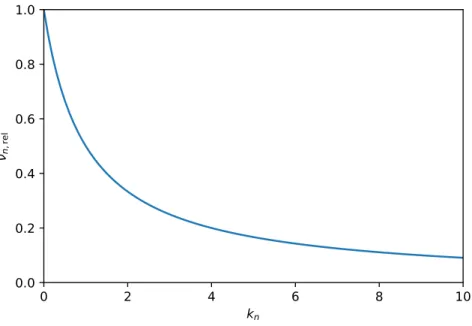
In Fig. 1.4,ν_n,rel can be seen as a function of retention factor of the last eluting component.

It is obvious that the most peak capacities gained close to the hold up time of the column. As the analysis time increases, the rate of peak capacity production decreases remarkably. This

0 2 4 6 8 10

k

0.0 0.2 0.4 0.6 0.8 1.0

n,rel

Figure 1.4: Rate of peak capacity production relative to the initialνn.

is due to the fact that peaks become wider as their retention time increase as it is shown by Eq. (1.4). As the retention of compounds increases their migration velocity decreases and more and more time is necessary to elute one band from the chromatographic column.

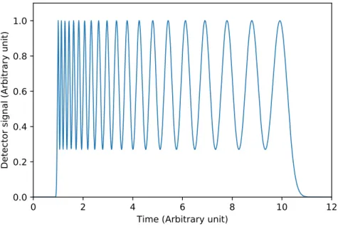
A 20-peak-capacity chromatogram can be seen in Fig. 1.5. The figure clearly shows the peak generation phenomenon discussed above. Most of the eluted peaks appear at the beginning of the chromatogram. Late eluting peaks are wider and more time is necessary to ensure unity resolution between them. Half of the total peak capacities generated in the first third of the analysis time. Figs. 1.4 and 1.5 emphasize the importance of reducing the retention of the first eluting peak. These figures also highlights the necessity of reducing extra column broadening since most of the peak capacities are generated in the beginning of analysis time. The narrow, early eluting peaks are more sensitive toward the detrimental effect of extra column processes.

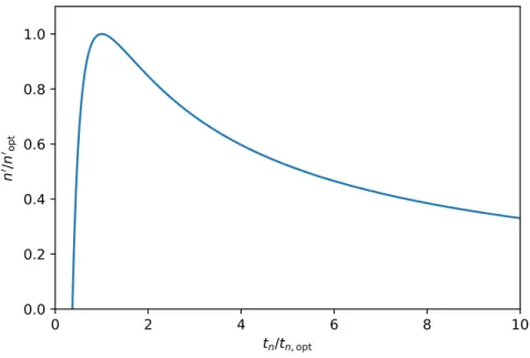
Specific peak capacity production,n⁰, shows how much total peak capacities generated in a given unit of time. It can be defined as

n⁰= n

t_n (1.28)

Specific peak capacity production has an optimum at t_n,opt=t₁exp

1− 4

√N

'2.718t₁ (1.29)

with a maximal value of

n⁰_opt= 1 t_n,opt

√N

4 '0.092

√N

t₁ (1.30)

0 2 4 6 8 10 12 Time (Arbitrary unit)

0.0 0.2 0.4 0.6 0.8 1.0

Detector signal (Arbitrary unit)

Figure 1.5: Chromatogram of a 20-peak-capacity separation in case of isocratic elution.

In Fig. 1.6, specific peak capacity production can be seen as a function of analysis time.

Note that the time axis is scaled fort_n,opt and the y axis is scaled for n⁰_opt. The figure clearly represent that the specific gain of peak capacity decreases by the increase of analysis time.

Accordingly, the analyst has to make a trade off between the the analysis time and separation power of the chromatographic system in the knowledge of the sample composition analyzed.

Plate number

A third option for the increase of peak capacity is the optimization of number of theoretical plates, N. In order to estimate column efficiency under different separation conditions, one should choose a proper plate height or plate number model. The most accurate equation for describing the dependence of the plate height on mobile phase linear velocity is offered by the general rate model. It is, however, so complex that it is rarely used in method development. The van Deemter and the Knox equations are the most widely used plate height equations in prac- tice. The simple form of the analytical solution for the minimum plate height obtained from van Deemter’s equation allows one to locate the optimum velocity and minimum plate height and to obtain insight into the contribution of kinetic processes to it. The Knox equation, however, provides better fit to liquid chromatography data than van Deemter equation. Therefore it will be used in the following.

Knox equation can be defined as

h=Aν

1

3 +B

ν +Cν (1.31)

0 2 4 6 8 10 t

/t

0.0 0.2 0.4 0.6 0.8 1.0

n

/n

Figure 1.6: Specific peak capacity production, Eq. (1.30), as a function of analysis time.

whereA,B, andCare dimensionless constant parameters. Their typical values are 0.8–1.0, 1.5, and 0.02–0.05, respectively,hthe reduced plate height that is the ratio of the height equivalent to a theoretical plate and the particle diameter,h=H/d_p, andν the reduced velocity.

ν = u₀d_p

D_m (1.32)

whereu₀ is the linear velocity of the mobile phase, d_p the particle size and D_m the diffusion coefficient of the solute molecules. Note that the reduced velocity is the same as the Péclet number used in study of transport phenomena.

An obvious way of peak capacity optimization in isocratic chromatography is the mini- mization of Eq. (1.31). Unfortunately, the exact solution of the minimum plate height based on Knox equation is too complicated to be informative. In Listing 1.2, however, a simple Python code is presented for obtaining the parameters of Knox plate height equation, and the optimal eluent velocity.

As it was discussed in the introduction, a popular approach of characterization and compari- son of column performances is the use of Poppe plots. In a single graph, it includes information on the plate number, the analysis time, and the maximum pressure that can be applied with the chromatographic system. Therefore, it is more capable for optimization purposes than a single plate height equation. In a Poppe plot, the plate time (H/u₀orN/t₀) is plotted against separa- tion efficiency. During the construction of these plots it is assumed that the chromatographic system is operated at the maximum allowed pressure, ∆P. The latter can be described by the

#-#-#-# Use with Listing 1.1 #-#-#-#

#Experimental data. Replace with actual data!

#eluent linear velocities, m/s

u0s = np.array([9.62e-05, 1.443e-04, 1.924e-04, 2.405e-04, 3.849e-04,\

4.811e-04, 9.623e-04, 1.4435e-03, 1.9247e-03, 2.4059e-03,\

2.8871e-03, 3.3683e-03, 3.8495e-03, 4.3307e-03, 4.8119e-03,\

5.2931e-03, 5.7743e-03, 6.2555e-03, 6.7367e-03, 7.2179e-03,\

7.6991e-03, 8.1802e-03])

#number of theoretical plates at u0s eluent velocities

Ns = np.array([3377.5, 4773.7, 6232.9, 7110.8, 9453.8, 11123.4,\

14019.4, 14868.8, 14336.9, 13828.5, 13666.4, 12903.1, 12553.7,\

12279.4, 11725.8, 11183.2, 11100.6, 10710.1, 10196.1, 10023.4,\

9899.3, 9699.0])

dp = 1.7e-6 #particle diameter, m L = 0.05 #column length, m

nus = u0s*dp/dm #eluent reduced velocities

Hs = L/Ns #heights equivalent to a theoretical plate, m

fp, fcv = curve_fit(h, u0s*dp/dm, Hs/dp) #fitting Knox equation on experimental data A, B, C = fp[0], fp[1], fp[2] #parameters of Knox equation

print('A = {0:.3f}, B = {1:.3f}, C = {2:.3f}'.format(A, B, C)) #print results

opt = minimize(h, 2, args=(A, B, C)) #minimize Knox equation with parameters A, B, C print('Minimum reduced HETP: {0:.3f}, minimum HETP: {1:.3f} um'\

.format(opt.fun, opt.fun*dp*1e6)) #print minimum HETP

print('Optimal reduced velocity: {0:.3f}, optimal velocity: {1:.3f} cm/min'\

.format(opt.x[0], opt.x[0]*dm/dp*100*60)) #print optimal velocity

Listing 1.2: Python code for determination of parameters of Knox plate equation.

∆P= φu₀ηL

d²_p (1.33)

whereLis the column length,η the dynamic viscosity of the eluent, andφ the column resis- tance factor which is in the range of 500–1000 (1000 is assumed in this work).

Considering that the column length,L, is the product of the required plate count,N_req, and the plate height (that ish d_p), Eq. (1.33) can be rewritten as

∆P= φu₀ηN_reqh

d_p (1.34)

From Eq. (1.34) it is possible to calculate the maximal plate number generated when the column work at the optimal eluent velocity.

N_opt= d²_p∆P

ν_minD_mη φh_min (1.35)

whereh_minis the minimum reduced plate height obtained atν_minoptimal reduced eluent veloc- ity.

The column length necessary to generateN_optplate numbers is

L_opt=N_opth_mind_p= d³_p∆P

ν_minD_mη φ (1.36)

with a dead time of

t_0,opt= N_opt² h²_minη φ

∆P = d⁴_p∆P

ν_min² D²_mη φ (1.37)

Note that Eq. (1.35) is not the maximum plate number that can be generated by the given stationary phase. N_opt is the maximum achievable plate count when the column is operated at the optimal eluent velocity and the column length is maximized in order to reach∆P. The overall maximum of plate number is

N_max= d²_p∆P

B D_mη φ (1.38)

where B is a parameter of the plate height equation Eq. (1.31). If van Demter equation is used to estimate column efficiency,N_maxbecomes the same mathematically as in case of Knox equation. Considering the typical values ofB, ν_min andh_min, it can be predicted thatN_max is

∼3-times larger than N_opt. This observation serves with the important conclusion that plate number can be further increased by using longer columns even if the eluent velocity becomes smaller than the optimal one.

The minimum reduced plate height of a well packed column is∼2.0 in case of fully porous, and∼1.7 in case of core-shell phases with optimal reduced flow rate 2.0–3.0. Assuming that ν_min is 2.8, N_opt of a column packed with 1.7µm fully porous particles operated at 1200 bar pressure is 62 000 for small molecules (D_m=10⁻⁹cm²/sec). A 21 cm long column with a slightly more than 2 min dead time is necessary to obtain this separation performance. For 5µm particles and 400 bar pressure drop, N_opt is larger, ∼180 000. This efficiency can be generated with a 1.8 m long column and 53 min dead time.

Eqs. (1.35)–(1.38) serve with important conclusions. The achievable plate number is di- rectly proportional to the applied pressure and to the square of particle diameter. Accordingly, the larger particles used, the higher plate number can be generated by the chromatographic sys- tem. A two-fold increase ofd_pcan produce four-times more plates. It was shown in Eq. (1.8) that the peak capacity is proportional to the square root of N. Therefore, n is directly pro- portional to the particle diameter and to the square root of pressure of separation. One can generate more peak capacities by using larger particles and higher operating pressures. In the same time, however, the time of analysis increase with the fourth power ofd_p. It means that a two-fold increase of peak capacity requires 16-times more analysis time and an 8-times more longer column if the peak capacity is increased by the duplication of particle size. The same improvement can be achieved by the quadruplication of the pressure. In that case both the anal- ysis time and column length are quadrupled. Note that these conclusions are valid numerically only for columns operated at the optimal eluent velocity. The tendencies, however, are valid in any eluent conditions.

In Eq. (1.35) there is no column length. The idea behind Eq. (1.35) is that the column work at the optimal flow rate that produces the minimal plate height. The column length is adjusted in order to generate the maximal pressure drop, ∆P. In the construction of Poppe plots, the same approach can be used with the difference that the eluent velocity is varied in order to generate the required plate number. The following equation is solved forν

∆P d_p

φ ηN_req−νD_m

d_p h=0 (1.39)

Note thathis a function ofν.

The plate height, plate number, column length and dead time are calculated by the appro- priate substitutions into Eqs. (1.31) and (1.35)–(1.37). By plottingH/u₀orN/t₀againstN_req, the Poppe plot can be constructed.

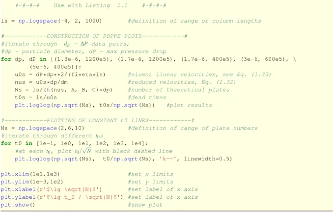
A simplified approach for the construction of Poppe plot is to vary column length in a wide range. It defines the value ofu₀ from Eq. (1.33). u₀allows the calculation of plate height by Eq (1.31), then the plate number asL/H, and the dead time asL/u₀. By plottingN/t₀against N_req, the Poppe plot can be constructed. In Listing 1.3, this simplified approach is presented for

ls = np.logspace(-4, 2, 1000) #definition of range of column lengths

#---CONSTRUCTION OF POPPE PLOTS---#

#iterate through d_p - ∆P data pairs,

#dp - particle diameter, dP - max pressure drop

for dp, dP in [(1.3e-6, 1200e5), (1.7e-6, 1200e5), (1.7e-6, 400e5), (3e-6, 600e5), \ (5e-6, 400e5)]:

u0s = dP*dp**2/(fi*eta*ls) #eluent linear velocities, see Eq. (1.33) nus = u0s*dp/dm #reduced velocities, Eq. (1.32)

Ns = ls/(h(nus, A, B, C)*dp) #number of theoretical plates

t0s = ls/u0s #dead times

plt.loglog(np.sqrt(Ns), t0s/np.sqrt(Ns)) #plot results

#---PLOTTING OF CONSTANT t0 LINES---#

Ns = np.logspace(2,6,10) #definition of range of plate numbers

#iterate through different t₀s

for t0 in [1e-1, 1e0, 1e1, 1e2, 1e3, 1e4]:

#at each t0, plot t0/√

N with black dashed line

plt.loglog(np.sqrt(Ns), t0/np.sqrt(Ns), 'k--', linewidth=0.5)

plt.xlim(1e1,1e3) #set x limits

plt.ylim(1e-3,1e2) #set y limits plt.xlabel(r'$\lg \sqrt{N}$') #set label of x axis plt.ylabel(r'$\lg t_0 / \sqrt{N}$') #set label of x axis

plt.show() #show plot

Listing 1.3: Python code for construction of Poppe plot.

the construction of Poppe plot. It can be seen that this approach does not need any numerical optimization algorithm.

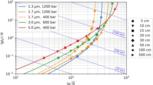
In Fig. 1.7, Poppe plot of different diameter column packings can be seen. The pressure drop is varied according to the typical maximum pressure used with these particles. Since square root of N is required for the estimation of isocratic peak capacities, t₀/√

N is plotted against√

N in the figure. Since the value of ^ln(1+δ)₄ in Eq. (1.8) is close to unity under most of the practically relevant conditions (δ >15), Fig. 1.7 can be considered as a kinetic plot of isocratic peak capacities. The diagonal lines represent zones of constant analysis times.

Fig. 1.7 demonstrates clearly that, in the practically relevant range of analysis times (t₀=10−100 sec), higher peak capacities can be generated with columns packed by smaller packing material than by larger ones provided that each column is operated at the highest al- lowed pressures. Similarly, it is possible to achieve the same peak capacity in significantly shorter analysis times by applying ultra-high performance stationary phases. The advantages of larger particle sizes arose when the goal is to produce very high peak capacities (>500). The vertical asymptotes correspond to the square root of maximal plate counts as it is calculated by Eq. (1.38). As it can be seen, with the use of larger particles higher peak capacities can be achieved. The cost of this separation power is the extremely large analysis time, however. The figure also emphasize that the use of 1.7µm particles in a 400-bar HPLC system does not offer

10¹ 10² 10³ lg N

10 ² 10 ¹ 10⁰ 10¹ 10²

lgt0/N

10 sec 100 sec 1000 sec

1.3 m, 1200 bar 1.7 m, 1200 bar 1.7 m, 400 bar 3.0 m, 600 bar 5.0 m, 400 bar

5 cm 10 cm 15 cm 20 cm 30 cm 50 cm 100 cm 500 cm

Figure 1.7: Poppe plot of isocratic peak capacity. Parameters of calculations: maximal pres- sure drop∆P=400 bar, viscosityη=0.001 Pa s, flow resistance factorφ=1000, diffusion coeffi- cientD_m=10⁻⁹m/s, reduced plate height expression Eq. (1.31) with parametersA=1.0,B=1.5, C=0.05 [7].

significant improvement over larger particles in the practically relevant range of analysis times.

In general, it can be concluded that when time is not a limiting factor, the peak capacity of an isocratic separation can be maximized by the increase of retention window and the use of large particles and the longest possible columns consistent with the pressure limit of the instrument.

Even if Poppe plot allows detailed comparison of different stationary phases and separation strategies, most of the points on the curves do not have any practical relevance. No one has, e.g., a 17.9 cm long column packed with 5µm particles to generate 8 000 plates. Instead, there are one or more 5, 10, and 15-cm long columns in the drawer. In Fig. 1.7, points calculated for column lengths that are possible to combine from commercially available columns are also presented. These points present the practically relevant separation conditions. By use of these points one can easily compare different separation strategies and decide the most appropriate one considering the required peak capacity and the available instrumentation and consumables present in the analytical lab.

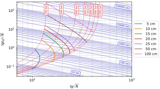
A more complete design and optimization of isocratic separation can be achieved by con- structing nomogram-like Poppe plots, as it is shown in Fig. 1.8. This figure is calculated for 1.7µm particles. Red dashed lines represents pressure drops, blue dashed lines the column hold-up times, and thick color lines some typical column lengths that can be combined by con- necting commercially available columns. Fig. 1.8 gives a deep insight into the influence of chromatographic conditions on the achievable separation power. It can be concluded that by increasing the column length the plate number can be improved even if∆P remains constant.

10² 10³ lg N

10 ¹ 10⁰ 10¹ 10²

lgt0/N

10 sec

100 sec 1000 sec 10000 sec

100 bar 200 bar 400 bar 600 bar 800 bar 1000 bar 1200 bar

5 cm 10 cm 15 cm 20 cm 25 cm 50 cm 100 cm

Figure 1.8: Nomogram for the design and optimization of isocratic separation with 1.7µm particles. Parameters of calculation can be found in caption of Fig. 1.7.

The increase of ∆Palways decrease the plate time, even ifN might decrease since the eluent velocity exceed the optimal one. When the columns are short, it is advantageous to operate the column at the optimal flow rate. At large columns, maximal∆Pis smaller than that would be necessary to produce that eluent flow rate.

Nomograms such as Fig. 1.8 can be used in method development directly. First, the analyst should define the maximal pressure drop applicable. Then, moving along the “isobar”, the column length that produce the desired plate count in an acceptable analysis time can be found.

One can generate nomograms like Fig. 1.8 for any phases available in the lab. The optimal column dimensions, stationary phases and operating conditions can be selected directly by the comparison of these nomograms.

In Listing 1.4, a Python code is presented for the generation of nomogram-like Poppe plots.

Note that the import of NumPy and Matplotlib packages, the definition of reduced plate height equation and some constant parameters are not included in Listing 1.4. Those can be found in Listing 1.1. Therefore the two codes should be used together in order to generate the nomo- gram.

1.3.2 Optimization of gradient separations

Extra column broadening

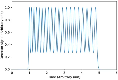
It was shown previously, that extra column band broadening has a detrimental effect on achiev- able peak capacities in isocratic elution. In Fig. 1.9, a typical 20-peak-capacity chromatogram of gradient separation is shown. The timescale is the same as in Fig. 1.5. It can be seen, that the

#-#-#-# Use with Listing 1.1 #-#-#-#

dp = 1.7e-6 #definition of particle diameter, m

#---CONSTRUCTION OF "ISOBARS"---#

ls = np.logspace(-4,2, 1000) #definition of range of column lengths

#iterate through different pressure drops

for dP in [100e5, 200e5, 400e5, 600e5, 800e5, 1000e5, 1200e5]:

u0s = dP*dp**2/(fi*eta*ls) #eluent velocity, m/sec, see Eq. (1.33) Ns = ls/(h(u0s*dp/dm, A, B, C)*dp) #plate numbers

t0s = ls/u0s #column hold up times, sec

plt.loglog(np.sqrt(Ns), t0s/np.sqrt(Ns), 'r--', linewidth=0.5) #plot isobars

#---PLOTTING OF CONSTANT t0 LINES---#

Ns = np.logspace(2,6,1000) #definition of range of plate numbers

#iterate through different t₀s

for i in [1e-1, 1e0, 1e1, 1e2, 1e3, 1e4, 1e5]:

#at each t0, plot t0/√

N with blue dashed line

plt.loglog(np.sqrt(Ns), i/np.sqrt(Ns), 'b--', linewidth=0.5)

#---CONSTRUCTION OF POPPE CURVES FOR DIFFERENT COLUMN LENGTHS---#

dP = np.logspace(7,np.log10(1200e5), 1000) #definition of pressure range, Pa

#iterate through different column lengths that has practical relevance for length in [0.05, 0.1, 0.15, 0.2, 0.25, 0.5, 1]:

u0s = dP*dp**2/(fi*eta*length) #eluent velocity, m/sec, see Eq. (1.33) Ns = length/(h(u0s*dp/dm, A, B, C)*dp) #plate numbers

t0s = length/u0s #column hold up times, sec

plt.loglog(np.sqrt(Ns), t0s/np.sqrt(Ns)) #plot Poppe curves in log-log scale

plt.xlim(70,1e3) #set x limits

plt.ylim(1e-2,1e3) #set y limits plt.xlabel('$\lg \sqrt{N}$') #label of x axis plt.ylabel(r'$\lg t_0 / \sqrt{N}$') #label of y axis

plt.show() #show plot

Listing 1.4: Python code for construction of nomogram-like isocratic Poppe plot.

0 1 2 3 4 5 6 Time (Arbitrary unit)

0.0 0.2 0.4 0.6 0.8 1.0

Detector signal (Arbitrary unit)

Figure 1.9: Chromatogram of a 20-peak-capacity separation in case of gradient elution.

same peak capacity could be generated in much less time. The peaks in Fig. 1.9 remain nar- row throughout the whole separation range. Accordingly, in gradient elution the extra column effects should be more significant than in isocratic runs.

In Fig. 1.10, the relative decrease of peak capacities are shown for a 50×2.1 mm column packed with 1.7µm particles and a 150×4.6 mm column packed with 5µm particles as a func- tion of volumetric extra column variance. Note, that typical values of extra column variances of UHPLC, optimized HPLC, and non-optimized HPLC systems are 5, 25, and 100µL²[17, 18], respectively. Fig. 1.10 emphasize the necessity of minimizing extra column volumes of chro- matographic system. Even a state of the art chromatograph can decrease the peak capacity of an ultra-high performance column by 10%. The use of these columns in an obsolete hardware is senseless practically. Even a system with 20µL² extra column variance – that corresponds to a well optimized conventional HPLC or even some UHPLC systems – might decrease n by 20–40%. For large columns, with large dead volumes, the effect of system volume is less detrimental.

Gradient conditions

Optimization of conditions of gradient separations is a much more complex task than that of isocratic separations. Some of the parameters affecting peak capacity of gradient runs are not mutually independent. Therefore, numerical algorithms should be used in order to find the optimal separation conditions.

Since Poppe plot can be applied directly in isocratic method development (see Fig. 1.8),

0 20 40 60 80 100 120

2V,ext

0.3 0.4 0.5 0.6 0.7 0.8 0.9 1.0

Relative peak capacity

S = 5, lgk

= 2.46 S = 10, lgk

= 3.59 S = 15, lgk

= 4.83 S = 20, lgk

= 6.12

Figure 1.10: Relative decrease of gradient peak capacity as a function of extra column vari- ance. Solid lines: 50×2.1 mm column packed with 1.7µm particles (H= 2.81), dashed lines:

150×4.6 mm column packed with 5µm particles (H= 2.97).

it would be useful to apply the same concept in gradient runs as well. There are several ap- proaches to construct gradient kinetic plots [9, 20–24]. Here, we use Eq. (1.19) as the basis of calculations. Since gradient peak capacity is calculated by integrating 1/w(t) betweent₀ and the retention time of the last eluting compound,t_n, application of Eq. (1.19) requires thatt_nbe equal to the sum of gradient and hold up times,t_n=t₀+t_G. It ensures that the last compound elutes exactly at the time when the gradient leaves the column. This scenario can be called as an “utterly utilized gradient”. By rearranging Eq. (1.13),t_Gcan be calculated by the following equation.

t_G=k_ϕ0 S t₀∆ϕ

exp(S∆ϕ)−1 (1.40)

A simple strategy to construct gradient Poppe plot (Listing 1.5) is varying column length in a relatively wide range while particle diameter of the stationary phase, d_p, initial eluent concentration,ϕ₀, and the change of eluent composition,∆ϕ, are set constant. At each column length, the maximal eluent velocity,u_0,max, is calculated. It defines the values of plate height, H, and column hold-up time,t₀. The gradient time,t_Gis determined by Eq. (1.40). Finally, the peak capacity of the separation is calculated by Eq. (1.19) at each column length. By plotting the peak time,t_peak, against peak capacity, one can construct the gradient Poppe plot. Peak time is the ratio of total analysis time and peak capacity.

t_peak=t_G+t₀

n (1.41)

fi0, dfi = 0.05, 0.7 #initial eluent composition, change of eluent composition k0, S = 1e6, 20 #parameters of linear solvent strenth model, Eq. (1.12)

#retention factor of the last eluting compound at the beginning of analysis kfi0 = k0*np.exp(-S*fi0)

#---PLOTTING OF CONSTANT tg+t0 LINES---#

pcs = np.logspace(1,3,10) #definition of range of peak capacities

#iterate through different t₀+tG values for tgt0 in [1e1, 1e2, 1e3, 1e4, 1e5]:

#at each t₀+t_G, plot (t₀+t_G)/n with blue dashed line plt.loglog(pcs, tgt0/pcs, 'b--', linewidth=0.5)

#---CONSTRUCTION OF GRADIENT POPPE CURVES FOR DIFFERENT COLUMN LENGTHS---#

ls = np.logspace(-3,1,100) #definition of range of column lengths

#iterate through different d_p - ∆P data pairs,

#dp - particle diameter, dP - max pressure drop, c - color, m - linestyle for dp, dP, c, m in [(1.7e-6, 1200e5, 'C0', '-'), (1.7e-6, 400e5, 'C0', '--'), \

(3e-6, 600e5, 'C1', '-'), (3e-6, 400e5, 'C1', '--'), (5e-6, 400e5, 'C2', '-')]:

u0s = dP*dp**2/(fi*eta*ls) #eluent linear velocities Hs = h(u0s*dp/dm, A, B, C)*dp #plate heights

t0s = ls/u0s #column hold-up times

tgs = kfi0*S*dfi*t0s/(np.exp(S*dfi)-1) #gradient times, see Eq. (1.40)

pcs = peakcap(tgs, fi0, dfi, t0s, Hs, ls, S, k0) #peak capacities, see Eq. (1.19)

#plot curves in log-log scale with 'm' linestyle, 'c' color. Add label to legend.

plt.loglog(pcs, tgs/pcs, m, color=c, \

label=r'{0:1.1f} $\mu$m, {1:4.0f} bar'.format(dp*1e6, dP*1e-5))

plt.xlim(30, 1000) #set x limits

plt.ylim(0.1,500) #set y limits

plt.xlabel('Gradient peak capacity, $n$') #label of x axis plt.ylabel(r'$(t_G+t_0)/n$') #label of y axix

plt.legend() #show legend

plt.show() #show plot

Listing 1.5: Python code for construction of gradient Poppe plot shown in Fig. 1.11.

Note that in the construction of gradient Poppe plot, the column hold-up time should be taken into consideration.

Fig. 1.11 shows gradient Poppe plots of columns operated at different pressures and packed with different particles sizes. For the sake of comparability, the same viscosity and diffusion coefficient were used for the calculations as in Figs. 1.7 and 1.8 even if the appliedk₀(10⁶) and Svalues (20) suggest large molecule, such as large peptide. The trends shown in Fig. 1.11 are similar to the plots in Figs. 1.7. In the practical range of analysis times and column lengths, higher peak capacities can be achieved by using columns packed by smaller particles so long as the maximum operating pressure applicable to the phase is applied. Even if low pressure is used, ultrahigh-performance particles can provide higher rate of peak capacity production and faster analysis than larger particles. The vertical asymptotes of curves presented in Fig. 1.11 correspond to the maximal achievable peak capacities as they are calculated by Eq. (1.22). It can be seen that long columns packed by large particles can provide very high peak capacities, even if it takes high analysis times. The application of large pressures provides higher peak

10² 10³ Gradient peak capacity, n

10 ¹ 10⁰ 10¹ 10²

(tg+t0)/n

100 sec 1000 sec 10000 sec

1.7 m, 1200 bar 1.7 m, 400 bar 3.0 m, 600 bar 3.0 m, 400 bar 5.0 m, 400 bar

5 cm 10 cm 15 cm 20 cm 30 cm 50 cm 100 cm 500 cm

Figure 1.11: Poppe plot of gradient peak capacity for columns operated at different pressures and packed with different particles sizes. Parameters of calculations: k₀ = 10⁶, S = 20, ϕ = 0.05,∆ϕ = 0.7,D_m= 10⁻⁹m²/sec,η = 0.001 Pa sec,φ = 1000.

capacities and faster separations. It is desirable to use a column at the highest applicable flow rate in order to generate the highest peak capacity possible. These conclusions are in agreement with the isocratic Poppe plots.

Comparison of Figs. 1.7 and 1.11 emphasize the obvious conclusion that gradient separa- tions superior over isocratic ones. It was shown that√

Nin Fig. 1.7 corresponds to the isocratic peak capacity. Therefore, the figures can be compared directly. It can be seen that a∼1000 sec separation can generate 200–400 peak capacities in gradient run. The dead-time required to achieve the same order of nin isocratic separation is also∼1000 sec. Considering, however, that the total analysis time of an isocratic run is 20–40 times larger than thet₀ when the goal is to reach high separation power, it is indisputable that much higher peak capacities can be generated in much shorter time by gradient separation than by isocratic mode.

Eq. (1.19) shows that gradient steepness,b, is an important factor that influences separation power significantly. b consists of four parameters. S is fixed in the approach used here. t₀ is defined by the column length and pressure drop (throughu_0,max). The gradient time and change of eluent composition are not mutually independent parameters. Constrain shown in Eq. (1.40) defines their strict relationship. In Fig. 1.11, value of∆ϕ was set to 0.7. It is obvious that this artificially chosen parameter cannot serve with the optimal peak capacities and peak times. The proper choice oft_Gand∆ϕ is essential in the optimization of gradients. Both too steep and too shallow gradients are detrimental to the achievable peak capacity. Therefore, it is necessary to apply an optimization method for the determination oft_Gand∆ϕ.

Fig. 1.12 presents a nomogram-like gradient Poppe plot constructed for 1.7µm particles,

10² 10³ Gradient peak capacity, n

10 ¹ 10⁰ 10¹ 10

(tg+t0)/n

10 sec 100 sec

1000 sec 10000 sec 0.4

0.5

0.7 = 0.8 0.75

5 cm 10 cm 15 cm 30 cm 50 cm 100 cm

Figure 1.12: Nomogram for the support of optimization of gradient peak separation. For pa- rameters of calculations see Fig. 1.7

1200 bar max. pressure drop, and column lengths that have practical relevance. The figure is similar to Fig. 1.8. It can also be used directly in method development. By using Fig. 1.12, one can find the separation conditions that (1) offer the highest peak capacity in a given analysis time, or (2) requires the shortest time to generate a given peak capacity. In the first case sce- nario, the analyst should move on the straight line of target analysis time (dashed blue lines on the figure) to find the column length,L, that offer the highest peak capacity. The dead time can be determined from the column length and pressure drop applied in the analysis by rearranging Eq. (1.33) for u₀. Gradient time, t_G is given as the difference of total analysis time and t₀. The required change of eluent composition can be determined either by interpolating between the iso-∆ϕ lines (dashed red lines on the figure), or by calculating it from Eq. (1.40). Since Eq. (1.40) cannot be rearranged to calculate∆ϕ directly, a proper root finding algorithm, such as the following, is necessary for the calculation of its value:

dfi = brentq(lambda dfi: trgrad(tg, fi0, dfi, t0, S, k0)-(t0+tg), 1e-6, 1-fi0)

Here we took Brent’s method provided by SciPy scientific computing library to find∆ϕ where the retention time of the last eluting compound is equal to the sum of column hold-up time and gradient time. The bracketing values of∆ϕ required by Brent’s method were chosen as 10⁻⁶ and 1−ϕ0since∆ϕ should be larger than zero and smaller than or equal to 1−ϕ0.

In the second case scenario, the analyst first should find the column that offer the target peak capacity in the shortest analysis time. It can be determined from Fig. 1.12 directly. The eluent velocity is given by Eq. (1.33). The dead time can be determined as L/u₀. The total analysis time is given as the product of n and peak time,(t_G+t₀)/n. Then, gradient time is given as the difference of total analysis time andt₀. ∆ϕ can be determined as it was shown in