THE IMPORTANCE OF BEHAVIOURAL FACTORS FOR PENSION SAVINGS DECISIONS –
CROSS-COUNTRY EVIDENCE
a, b, cAnna KALICIAK – Radosław KURACH – Walid MEROUANI (Received: 13 February 2018; revision received: 18 July 2018;
accepted: 6 August 2018)
In this study, we challenge the problem of inadequate voluntary pension savings by exploring the micro-dataset of the Luxembourg Wealth Study (LWS) for three countries: Italy, the United King- dom and the United States. The existing empirical literature usually focuses on the role of socio- demographic factors to understand this phenomenon, and theoretical studies additionally highlight the role of behavioural factors. However, empirical studies in this fi eld are extremely scarce. The use of the LWS data enables us to fi ll this research gap. Separately for each country, we verify the role of individuals’ risk attitudes and intertemporal choices in the demand for voluntary pension savings. To make the results more robust, we add a set of socio-demographic control variables to our regressions. Our fi ndings clearly reveal that being more risk averse and being less forward look- ing negatively affect people’s propensity to save for retirement. Furthermore, we confi rm that age, gender and education are signifi cant predictors of pension demand in each of the analysed coun- tries. We argue that these conclusions have practical meaning to improve regulatory frameworks.
Keywords: supplementary pension savings, risk aversion, intertemporal choices, socio-demo- graphic factors, Tobit models
JEL classifi cation indices: C25, G41, J32
a) We are thankful to Jeffrey R. Brown, Christos Koulovatianos, Maureen Maloney, Edyta Marcinkiewicz and Piotr Paradowski for their constructive remarks on the earlier version of this manuscript. We would also like to acknowledge the participants of the 2nd Old-Age Security Con- ference (Wrocław, 2016) and the LIS/LWS Users Conference (Belval Campus, Luxembourg, 2017) for their encouragement. Last but not least, the insightful comments made by the anonymous re- viewers are much appreciated. All remaining errors are our own.
b) The research was supported under the European Commission’s 7th Framework Programme (FP7/2013-2017, grant No. 312691).
c) The preliminary results have been also published in LWS Working Paper Series, No. 23, 2016.
http://www.lisdatacenter.org/wps/lwswps/23.pdf
Anna Kaliciak, PhD student, University of London, United Kingdom.
E-mail: anna.kaliciak@city.ac.uk
Radosław Kurach, corresponding author. Assistant Professor at Faculty of Economic Sciences, Wrocław University of Economics, Poland. E-mail: radoslaw.kurach@ue.wroc.pl
Walid Merouani, Researcher at Centre de Recherche en Économie Appliqué pour le Développe- ment (CREAD, Algeria) and Centre de Recherche en Economie et Management (CREM-CNRS, France). E-mail: merouaniwalid@hotmail.fr
1. INTRODUCTION
Due to society’s ageing process, the replacement rate in the public pension system is expected to steadily decrease in the coming decades. However, a reduction in consumption opportunities faced by future pensioners may not be politically ac- ceptable. Therefore, to avoid the additional redistribution from the working-age generation to the pensioners, one of the available solutions for government is to make an effort to motivate individuals to accrue supplementary savings for their retirement. The current international experiences are not optimistic, as participa- tion rates are often far from the satisfactory (Rutecka et al. 2014).
The existing literatures usually try to explain the observed heterogeneity in the demand for voluntary pensions with socio-demographic determinants (Peeters et al. 2003; Stinglhamber et al. 2007). However, although the importance of the previously investigated factors is undeniable, this type of evidence does not pro- vide useful conclusions for economic policy. Relating pension decisions only to the socio-demographic characteristics would make it hard for government to successfully affect individuals’ decisions. Therefore, in this paper, we extend the list of potential determinants of this phenomenon with two behavioural variables – financial risk attitudes
1and intertemporal choices – whose importance for sav- ings decisions has been presented mainly on a theoretical basis (Samuelson 1937;
Yaari 1965; Bommier 2006). The empirical verification for the significance of the aforementioned behavioural factors addresses the question of whether and how policymakers can nudge people to save.
Our study contributes to the existing literature by delivering empirical evi- dence based on the updated data set from the Luxembourg Wealth Study 2016 (LWS) for three countries, i.e., Italy, the UK and the USA
2. LWS uses national surveys from the upper- and middle-income countries and homogenises them, providing a unique opportunity to run cross-country comparative studies. It ena- bles the formulation of not only country-level but also global-level conclusions and further policy recommendations.
The remainder of the paper is organised as follows: Section 2 presents the theoretical rationale for exploring the risk attitudes and intertemporal choices in analysing individuals’ retirement savings decisions. Section 3 surveys the empiri- cal literature and Section 4 presents the model and hypotheses tested. Section 5 contains a detailed description of the dataset used in this research. In Section 6, we report the empirical outcomes, and Section 7 concludes.
1 From now on referred to, for simplicity, as ‘risk attitudes’, ‘risk aversion’ or ‘risk tolerance’
interchangeably.
2 The sample has been narrowed down to three countries due to data availability on risk aver- sion and/or intertemporal choices in the LWS database.
2. THEORETICAL BACKGROUND
The individual decisions concerning pension savings for retirement are complex, involving a wide variety of determinants. Such problems can be analysed within two major dimensions: First, an individual decides how much money to save at each single point in time, and also controlling for the way of savings (type of financial product, time horizon, etc.). This perspective implies an analysis based on the portfolio selection criteria. That is, given a person’s current income, her at- titude towards risk and specific characteristics of the financial products available in the market, she makes an optimal decision regarding how to allocate the total money at her disposal. The aforementioned determinants come from the assump- tions underlying the commonly recognised model of modern portfolio theory (Markowitz 1952). Interestingly, an alternative model adds psychological traits as another powerful influential factor. The behavioural portfolio theory (Shefrin – Statman 2000) allows for such decisions to be adjusted for the cognitive errors individuals experience when assessing the probability distribution of future out- comes (returns) on particular financial opportunities. This assessment is affected, for example, by the common bias of overweighting the small probabilities of high returns while underweighting the high probabilities of low returns (or losses).
Second, it is essential to introduce time variation into retirement savings analy- sis. Any issue concerned with the pension topic is reviewed in the long run. The central point is a trade-off between current and future consumption, as individuals decide on what fraction of their income to spend today while saving the rest and delaying consumption until later (i.e. reaching the retirement age). When analys- ing the intertemporal choice problem the two core concepts are utility theory and time discounting (Camerer et al. 2003). Rational agents are assumed to discount the utilities obtained from possible future outcomes in the form of their expected values and then maximise over the set of such alternatives (Samuelson 1937).
Moreover, the agents are assumed to be risk averse on average. The problem with the expected utility theory, however, is that while many different shapes of utility functions have been proposed, none can be undoubtedly verified by observable decision making (Friedman – Savage 1948).
Time discounting, on the other hand, originates from the assumption that peo-
ple do not equally value cash flows that are the same in absolute terms but occur
at different points in time. People, who are more impatient, for example, exhibit
a higher rate of discount, meaning that the future value of money diminishes for
them very fast. Classically, an exponential form is used when assessing the dis-
counting function. However, this form implies an individually fixed rate of time
discounting, whereas experimental data suggest that people tend to behave in-
consistently in terms of discounting, by changing the rates as time passes (Thaler
1981). This is why it is increasingly important to introduce hyperbolic or quasi- hyperbolic discounting functions (Strotz 1955).
One of the most prominent theoretical frameworks in the context of intertem- poral choice is a life-cycle model. Its central assumption holds that individu- al consumption-savings decisions today are determined by the expectations of changes in future income. Specifically, it is believed that a person adjusts his current consumption level with respect to both current and anticipated future in- comes. For instance, according to the model, one would increase his spending today when faced with a reliable belief of receiving higher earnings tomorrow (Diamond – Hausman 1984). However, the assumptions of life-cycle theory in practice might not always work. People often tend to behave with a backward- instead of a forward-looking perspective (making their current decisions based on past actions), but they may also face particular constraints preventing them from increasing their current consumption.
3. SURVEY OF EMPIRICAL LITERATURE
The empirical research analysing the role of the investigated behavioural factors for pension decisions is scarce, but it confirms the need for further empirical verification in this particular area.
O’Donnell (2011) focused on the UK and Irish households employing the re-
sults of the surveys run by local regulators. In the first step, the obtained risk
aversion measures were regressed by the following socio-demographic charac-
teristics: ethnic background variables, age, region of residence, marital status,
gender, illness, the number of children under 18 years of age and the highest
educational attainment of the individuals. In both countries, people with an eth-
nic background, singles and women were found to be more risk averse. Further,
O’Donnell (2011) ran two types of models to explain the observed pension assets
holdings, first with only the socio-demographic exogenous variables and then
with the addition of proxies of risk attitude. But, the results were not conclu-
sive. Risk-tolerant households were more likely to collect pension assets, but the
estimated parameter was not significant, because the risk measure was highly
correlated with other socio-demographic factors. Clark et al. (2012) challenged
a specific research question about the reliance on home ownership for retirement
planning. Using the results of a unique survey from 2007, where 2,400 partici-
pants of a defined contribution pension plan that was offered by an investment
bank located in London were asked about their attitude to the role of home own-
ership, they compared the collected responses with the set of socio-demographic
characteristics and a few risk attitude measures. The first finding was that in-
dependent of the employed risk attitude proxy, the models estimated after the addition of one of these variables were better than the models that relied only on socio-demographic factors. Second, those individuals, who declared that they relied upon the family home for a ‘majority of their retirement needs’, were found to be highly risk averse.
We can also find researches investigating the significance of time preference (again: a trade-off between current and future consumption) for the decisions regarding pension savings. Munnell et al. (2001/2002), using the results of 1998 Survey of Consumer Finances, confirmed that people with a short planning ho- rizon were less likely to participate in a popular 401(k) plan in the US. Finke – Huston (2013) analysed the responses of nearly 7,000 students about the im- portance of savings for retirement. The intertemporal choices of the students were measured in two ways: The first was by measuring the time preference for money using a log-transformed numerical dollar comparison. The second was by asking a set of questions regarding eight behaviours that involve a trade-off between present and future utility. In conclusion, they confirmed the importance of both measures, but a scale of eight behaviours was found to be a better predictor of the importance of retirement savings than the traditional numerical scale of time preference. However, it should be noted that they analysed the self-reported state- ments of the students, which may not reflect their true savings decisions.
We contribute to the related research in two ways: First, we investigate simul- taneously the importance of two behavioural factors that should support the ro- bustness of the obtained results. Second, by using the internationally comparable LWS dataset, we try to indicate the country-specific and global determinants of demand for voluntary pensions.
4. OUR ECONOMETRIC APPROACH
To verify the link between behavioural variables and the demand for pension ac- counts, we estimate the following models for each country
3separately:
(1)
3 Estimating the model on a full dataset would be undesirable as the number of observations for each country varies significantly.
, ,
1 1
,
1 1
* *
* (1)
r z
i i i k i k i i j i j i
k j
s n
j i j i k k i
j k
PA RA IT SD RA IT SD IT
SD RA INT
γ θ μ δ
β ε
where
,
*
, 'k i j i j
INT SD SD (2)
and RA is a risk aversion variable, IT is an intertemporal choices variable, SD is a vector of j socio-demographic control characteristics, and PA is a pension account variable describing the demand for the voluntary pension savings of a particular individual, i.
The demand for pension (PA) is measured by the amount of funds accumulated in the individual voluntary pension account. The value of the accumulated assets can be equal to 0 for people who do not save at all or positive and continuous for the rest. Hence, we deal with a censored variable (censored from below). In our case, we use a Tobit model to explain two decisions simultaneously. The first decision is whether to save voluntarily, and in the case of a positive answer, the second decision is about how much to save. Hence, it is a combination of two models: probit and truncated regression.
In order to deliver more precise results, we decide to estimate the set of inter- action effects in our models. These interaction effects would measure the impact of two (or more) independent variables on the dependent variable. It is based on interpreting the μ, δ
j,
jand β
k. For example, the parameter (β
1) measures the impact of SD
i,jꞌon PA given the value of SD
i,j. For example, SD
i,jis a gender variable (0 for male, 1 for female) of an individual i, and SD
i,jꞌis a marital status dummy variable (1 if the individual married) for the same individual i. The in- teraction effect measured by β
1reflects the impact of being married on pension savings for females or for males. In our study, we have estimated the interaction between two investigated behavioural variables (RA
i IT
i), two interactions be- tween socio-demographic and behavioural variables, i.e. gender and risk aversion (SD
i,jRA
i) (s = 1) and gender and intertemporal choices (SD
i,jIT
i) (z = 1), and also five (n = 5) interactions between socio-demographic variables (SD
i,jSD
i,jꞌ), namely interactions between gender and education, immigrant status and income, age and education, education and income, and finally gender and marital sta- tus. These pairs have been chosen to test some literature findings. Hinz et al.
(1997) and Bajtelsmit – VanDerhei (1997) found that after controlling for income and age, women are more risk averse than men. Sundén – Surette (1998) identi- fied that among all married individuals, women are more risk averse than men.
Other studies have investigated interactions between a set of socio-demographic
variables and have found heterogeneous results (Lee – Hanna 1995; Adhikari –
O’Leary 2013).
5. DATA
The countries data applied in this study come from the “Survey on Italian House- holds’ Income and Wealth 2010” and “Household Assets Survey 2011” for the UK and “Survey of Consumer Finance 2013” for the USA. These three datasets have been further acquired and harmonised by Luxembourg Wealth Study 2016 (LWS) to enable comparability across these countries.
Each country has its specific dataset that contains two kinds of files: individu- al-level and household-level files. The individual files present information about household members, while the household files display information about particu- lar households. The total of the continuous variables for the household members is equal to the overall variable for this particular household; for example, the sum of the individual members’ income is reported as aggregate income in the house- hold file. Every file also contains a weight variable. The weight variable makes the sample representative for the overall population and hence allows for a more accurate estimation. The investigated variables have been standardised in terms of their content and coding structure. The continuous variables are expressed in the same units across different datasets. The categorical variables have been standardised and coded using the same value code and label for all countries.
We focus on three phenomena: risk aversion, intertemporal choices and de- mand for pensions. In the local surveys, risk aversion (RA) is measured asking the following question: “Which of the following statement comes closest to de- scribing the amount of financial risk that you (and your husband/wife/partner) are willing to take when you save or make investments?” The respondent can pick one of the following answers: (1) take substantial financial risks, expecting to earn substantial returns; (2) take above-average financial risks, expecting to earn above-average returns; (3) take average financial risks, expecting to earn average returns; and (4) not willing to take any financial risk. In the UK, the answers were ranked in 5 categories (see below) rather than four.
There are slight differences between the analysed countries in the assessment of intertemporal choices (IT). However, a comparison is still possible, as the results allow for classifying the individuals from the most patient ones (who do not discount the future) to the most impatient ones (who discount the future at the highest rate).
The set of questions to estimate time discounting rate measuring the intertem-
poral choices was as follows:
Italy: You have won the lottery and will receive a sum equal to your house- hold’s net yearly revenue. You will receive the money in a year’s time. However, if you give up part of the sum, you can collect the rest of your win immediately.
4Respondents were classified in 5 categories, from 1, the most patient (forward looking), to 5, the most impatient, as presented in Table 1.
Table 1. Intertemporal choice classifications for Italy (%) Category Agree to give up Refuse to give up
1 2
2 2 5
3 5 10
4 10 20
5 20
UK: If you had a choice of receiving a thousand pounds today or one thousand one hundred pounds next year, which would you choose?
1. £1,000 today; 2. £1,100 next year; 3. Don’t know/no opinion (Spontaneous only).
USA: In planning or budgeting your (family’s) saving and spending, which of the following time periods is most important to you (and your family living here):
1. The next few months; 2. The next year; 3. Next few years; 4. Next 5–10 years;
5. Longer than 10 years.
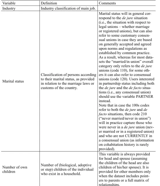
A detailed description of each socio-demographic regressors (SD) is found in Appendix A.
6. EMPIRICAL RESULTS
We start our verification procedure by analysing the diversity of the investigated samples with respect to the two behavioural variables.
4 This question can be considered as a measure of risk aversion: the amount that respondent is ready to give up to avoid future uncertainty is considered as a risk premium. However, in the question, the uncertainty about the future benefit is not mentioned. This is why we argue that the question measures patience (intertemporal choices): a respondent who is ready to give up more (20%) to get the amount immediately is considered as impatient.
We notice, unsurprisingly, that in every society, the majority of its members are moderately and highly risk averse (Table 2), which is in line with the empiri- cal outcomes reported by Barsky et al. (1997).
Table 2. Risk attitude by countries (%)
Italy USA UK
[1] takes substantial financial risks,
expecting to earn substantial returns 1.09 4.22 (1) Risk
tolerant 1
[2] takes above-average financial risks,
expecting to earn above average returns 19.71 18.95 2 8 [3] takes average financial risks, expecting
to earn average returns 33.11 39.96 3 16
[4] not willing to take any financial risk 46.09 36.87 4 45 (5) Risk
averse 30
Similarly, the summary statistics show the significant heterogeneity in people’s attitudes towards the future in the investigated countries. According to the tax- onomy presented in Table 1, 28% of the Italians are classified in the 1
stcategory, 16% in the 2
nd, 18% in 3
rd, 17% in the 4
thand 21% in the 5
th. In the UK, 76% of the respondents picked the immediate payment (1000 pounds today), 23% picked the deferred payment (1100 pounds next year), and 1% had no opinion. In the USA, 23% of the population was concerned about the next few months, 13% about the next year, 25% about the next few years, 23% about the next 5–10 years and 16%
about beyond the next 10 years.
The visual inspection of the statistics presented in Tables A.1, A.4 and A.6 does not provide a clear guidance about whether the behavioural factors are correlated with particular socio-demographic characteristics. The exception is the relation- ship between gender and risk attitude revealing that in every analysed country, women are more risk averse than men. However, the role of SD is assessed by estimating equation 1
5.
In every country, men are found to collect more in pension accounts than women
6. The first guess regarding the reason for this result could be gender wage
5 In Appendix B, we provide the models with those socio-demographic variables that were found to be significant.
6 We cannot directly interpret the estimates of the elasticity coefficients because in Tobit mod- els, they may be referred directly to the uncensored latent variable, not to the observed out- come. In other words, the estimated coefficients can be interpreted as the combination of change in the endogenous variable above the limit (in our case, the value of a pension account is greater than zero) weighted by the probability of being above the limit. Hence, we interpret only the coefficients’ signs and their significance.
gap, but we always include income as a variable in our models to account for it.
Another strong conclusion can be formulated about the role of education and fi- nancial literacy
7, which positively affect pension demand. In the case of Italy, an unexpected result is obtained regarding age, as this variable has a negative load.
This is probably due to the fact that in the past, the public pension system in Italy had provided relatively generous benefits, and government started to promote individual accounts only in 2007. We should also report the unique results regard- ing the ethnicity factor, which is verified only for the US due to data availabil- ity. All other ethnic groups, relative to “Whites (include Middle Eastern/Arabian with White); Caucasian”, were found to save less for retirement in individual accounts. To sum up, the identified significant relationships between the socio- demographic characteristics and pension demand justify the use of the SD vector as a set of control variables and should support the robustness of the conclusions on the role of risk attitudes and intertemporal choices.
The summarised results on the importance of the behavioural factors for pen- sion demand are presented in Table 3.
Table 3. Demand for pensions – summary results for behavioural predictors
Behavioural variable Italy UK USA
Risk aversion – – –
Intertemporal choice (being
forward looking) 0 + +
Note: ‘+’/‘–’ mean positive impact of a particular variable on pension demand, while ‘0’ indicates an insig- nificant variable. As the time preference factor for Italy is found to be insignificant, we estimate model 1 after excluding this variable.
We have identified that risk aversion negatively affects pension savings accu- mulation in each of the analysed countries (Tables A.3, A.5 and A.7). The observed negative relationship has also been confirmed by other studies (e.g. Bommier – Le Grand 2014). The potential explanation is that risk-averse individuals may be afraid of not receiving their savings back; hence, they tend to avoid uncertainty surrounding the future benefit and prefer current consumption.
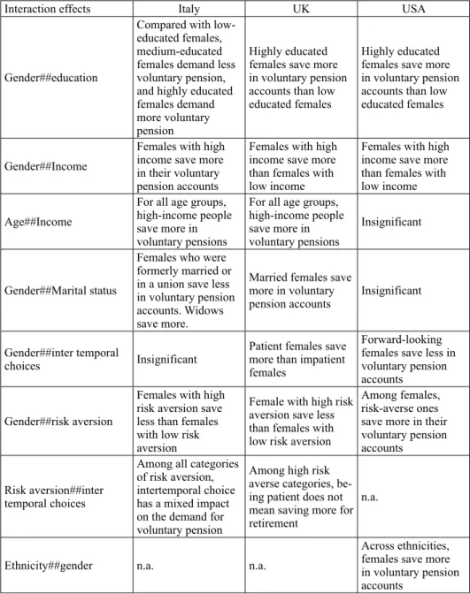
To deliver more detailed results, we have tested the interactions between the model variables, and the summary outcomes are displayed in Table 4.
When examining the interaction effects, we find that in Italy and the UK be- ing a woman intensifies the negative effect of risk aversion on pension demand.
Surprisingly, the opposite relationship is found for the USA, where risk-averse women save more than risk-tolerant ones.
7 The proxy for financial literacy was available only for Italy.
Table 4. Interaction effects when demand for pensions is the dependent variable
Interaction effects Italy UK USA
Gender##education
Compared with low- educated females, medium-educated females demand less voluntary pension, and highly educated females demand more voluntary pension
Highly educated females save more in voluntary pension accounts than low educated females
Highly educated females save more in voluntary pension accounts than low educated females
Gender##Income
Females with high income save more in their voluntary pension accounts
Females with high income save more than females with low income
Females with high income save more than females with low income Age##Income
For all age groups, high-income people save more in voluntary pensions
For all age groups, high-income people save more in voluntary pensions
Insignificant
Gender##Marital status
Females who were formerly married or in a union save less in voluntary pension accounts. Widows save more.
Married females save more in voluntary
pension accounts Insignificant
Gender##inter temporal
choices Insignificant Patient females save more than impatient females
Forward-looking females save less in voluntary pension accounts
Gender##risk aversion
Females with high risk aversion save less than females with low risk aversion
Female with high risk aversion save less than females with low risk aversion
Among females, risk-averse ones save more in their voluntary pension accounts
Risk aversion##inter temporal choices
Among all categories of risk aversion, intertemporal choice has a mixed impact on the demand for voluntary pension
Among high risk averse categories, be- ing patient does not mean saving more for retirement
n.a.
Ethnicity##gender n.a. n.a.
Across ethnicities, females save more in voluntary pension accounts
Note: n.a. = data are not available.
According to the existing literature (e.g. Arrondel et al. 2004; Lusardi – Mitch- ell 2007), people who highly discount the future should be less eager to save for retirement. Our study also supports this view for the UK (Table A.5) and the US (Table A.7), while in Italy, it is insignificant (Table A.2). Similar to the risk-aversion factor, in the case of intertemporal choices, we have also estimated its interaction with gender. However, the obtained results are inconclusive. Ad- ditionally, we have also tested the interaction between risk aversion and intertem- poral choices. The results show that in Italy, among all categories of risk aversion, being patient has a significant impact on voluntary pension savings; however, this result is somewhat noisy and difficult to read. The same mixed results have been obtained for the UK. In the USA, this interaction is not applied because the two variables are codified in four categories, which results in too many interactions.
Finally, in order to ensure the robustness of the obtained results we analysed Variance Inflation Factor (VIF) to test collinearity in all our models (Mansfield – Helms 1981). This phenomenon does not lead to biased estimates of the pa- rameters but may dramatically increase the probability of type II error – we may wrongly conclude that variable is insignificant. A commonly given rule of thumb is that VIFs of 10 or higher may be a reason of concern. In our study, the VIFs for all independent variables are substantially lower than the threshold which means that no collinearity problem exists in our models.
7. CONCLUSIONS
In this study we have demonstrated that the two investigated behavioural char- acteristics affect the demand for voluntary pensions in a similar way in the three analysed countries: Italy, the UK and the USA. We believe the obtained results enable us to formulate some policy recommendations to enhance people’s pro- pensity to save for retirement.
We have shown that, on average, greater risk aversion reduces people’s will-
ingness to save. An exception to the latter is the case of the USA, where the risk-
averse women were inclined to save more on average than those of higher risk
tolerance. Nevertheless, the majority of society members are at least moderately
risk averse, which should motivate the regulatory bodies to run a strict supervi-
sion of the pension saving sector. At the same time, financial institutions should
pay more attention to the development and sales of low-risk products, even if the
theory (Poterba – Summers 1988; Spierdijk et al. 2012) supports investing more
in risky instruments due to the mean reversion of their returns, which improves
the risk-return trade-off in the long run. High risk aversion may also have tre-
mendous consequences for the decumulation phase. Regulators should deeply
reconsider this argument whenever they wish to impose mandatory annuitisation of voluntary retirement savings. People may be afraid to die shortly after retir- ing
8; hence, they might have a feeling of overpaying the annuity. Therefore, the lump-sum option should always be available, and the longevity risk should be managed by the public (mandatory) pension pillar.
Our next general conclusion states that people who highly discount the future are less likely to save for retirement. Therefore, the government and/or private institutions should offer savings products combined with some other products/
services offering immediate benefits. Following Jhabvala (1998), examples from the public sector include access to the healthcare system for children of an in- sured person or discounted tickets for transportation. Clark et al. (2016) argue that something simple as a small incentive to attend a retirement workshop during individuals’ normal work hours may successfully change their behaviour.
Regarding the role of socio-demographic variables, we have found that age, gender and education are significant predictors of pension demand. Somewhat surprisingly, the analysis of “family variables”, i.e., marital status and number of children, does not drive us to any robust conclusions. This means that individuals in these analysed countries do not expect family support during old age. There- fore, this finding grounds the need for an institutional pension system.
According to the interaction effects, the impact of some variables on saving behaviours is different across gender, income, immigrant and age groups. These detailed results may also help project more effective policy solutions supporting saving for retirement in the diversified society.
Last but not the least, we should note the points that deserve further research attention. So far, we have investigated only two behavioural factors affecting the decision of pension savings, but the list of potential behavioural determinants is longer. One candidate may be an individual’s confidence in a public pension system. In the past few decades, especially in Continental Europe, governments were granting generous pension benefits (in terms of the replacement rate), as the demographic situation was favourable. Therefore, many people may recognise the current conditions as a “state of nature” and treat the warning consequences of demographic projections as incredible. Understanding the importance of these beliefs may have tremendous meaning for the future shape of pension systems.
8 Even if people systematically underestimate how long they will live (Drinkwater – Sondergeld 2004).
REFERENCES
Adhikari, B. – O’Leary, V. E. (2013): Gender Differences in Risk Aversion: A Developing Nation’s Case. Journal of Personal Finance, 10(2): 122–147.
Arrondel, L. – Masson, A. – Veger, D. (2004): Mesurer les préférences individuelles pour le présent (Measuring Individual Preferences for the Present). Economie et statistique, 374(1): 87–128.
Bajtelsmit, V. L. – VanDerhei, J. L. (1997): Risk Aversion and Pension Investment Choices. In:
Gordon, M. S. – Mitchell, O. S. – Twinney, M. M.: Positioning Pensions for the Twenty-First Century. Philadelphia: University of Pennsylvania Press, pp. 45–66.
Barsky, R. – Juster, T. – Kimball, M. – Shapiro, M. (1997): Preference Parameters and Behavioral Heterogenity: Experimental Approach in the Health and Retirement Study. The Quarterly Jour- nal of Economics, 112(2): 538–579.
Bommier, A. (2006): Uncertain Lifetime and Intertemporal Choice: Risk Aversion as a Rationale for Time Discounting. International Economic Review, 47(4): 1223–1246.
Bommier, A. – Le Grand, F. (2014): Too Risk Averse to Purchase Insurance? A Theoretical Glance at the Annuity Puzzle. Journal of Risk and Uncertainty, 48(2): 135–166.
Camerer, C. F. – Loewenstein, G. – Rabin, M. (2003): Advances in Behavioral Economics. Princeton and Oxford: Princeton University Press.
Clark, G. L. – Almond, S. – Strauss, K. (2012): The Home, Pension Savings and Risk Aversion:
Intentions of the Defi ned Contribution Pension Plan Participants of a London–Based Investment Bank at the Peak of the Bubble. Urban Studies, 49(6): 1251–1273.
Clark, R. L. – Hammond, R. G. – Khalaf, C. – Morrill, M. S. (2016): Planning for Retirement?
The Importance of Time Preferences. www4.ncsu.edu/~rghammon: ww4.ncsu.edu/~rghammon/
CHKM_PlanningPaper.pdf
Czeglédi, T. – Simonovits, A. – Szabó, E. – Tir, M. (2017): What is Wrong with the Hungarian Pen- sion Rules? Acta Oeconomica, 67(3): 359–387.
Diamond, P. A. – Hausman, J. A. (1984): Individual Retirement and Savings Behaviour. Journal of Public Economics, 23(1–2): 81–114.
Drinkwater, M. – Sondergeld, E. T. (2004): Perceptions of Mortality Risk: Implications for Annui- ties. In: Mitchell, O.S. – Utkus, S. P. (eds): Pension Design and Structure: New Lessons from Behavioral Finance. Oxford: Oxford University Press, pp. 275–286.
Finke, M. S. – Huston, S. J. (2013): Time Preference and the Importance of Saving for Retirement.
Journal of Economic Behavior & Organization, 89: 23–34.
Friedman, M. – Savage, L. J. (1948): The Utility Analysis of Choices Involving Risk. Journal of Political Economy, 56(4): 279–304.
Gale, W. G. (1998): The Effects of Pensions on Household Wealth: A Reevaluation of Theory and Evidence. The Journal of Political Economy, 106(4): 706–723.
Hinz, R. P. – McCarthy, D. D. – Turner, J. A. (1997): Are Women Conservative Investors? Gender Differences in Participant Directed Pension Investments. In: Gordon, M. S. – Mitchell, O. S. – Twinney, M. M.: Positioning Pensions for the Twenty-First Century. Philadelphia: University of Pennsylvania Press, pp. 91–106.
Jhabvala, R. (1998): Social Security for Unorganised Sector. Economic and Political Weekly, 33(22), L7–L11.
Lee, H. – Hanna, S. (1995): Empirical Patterns of Risk Tolerance. Proceedings: Academy of Fi- nancial Services.
Lusardi, A. – Mitchell, O. S. (2007): Financial Literacy and Retirement Preparedness: Evidence and Implications for Financial Education. Business Economics, 42(1): 35–44.
Luxembourg Wealth Study (2016) http://www.lisdatacenter.org (Italy, UK, USA; {April, 6th 2016–
April 19th 2016}). Luxembourg: LIS.
Mansfi eld, E. R. – Helms, B. P. (1981): Detecting Multicollinearity. The American Statistican, 36(3a): 158–160.
Markowitz, H. (1952): Portfolio Selection. Journal of Finance, 7(1): 77–91.
Munnell, A. H. – Sundén, A. – Taylor, C. (2001/2002): What Determines 401(k) Participation and Contributions? Social Security Bulletin, 64(3): 64–75.
O’Donnell, N. (2011): Analysing the Determinants of Attitudes to Risk and Their Role in Pension and Investment Decisions in Ireland and the UK. Central Bank of Ireland Quarterly Bulletin, April: 78–90.
Peeters, H. – Van Gestel, V. – Gieselink, G. – Berghman, J. – Van Buggenhout, B. (2003): Invisible Pensions in Belgium. https://perswww.kuleuven.be/: https://perswww.kuleuven.be/~u0032617/
downloads/Invisible%20pensions%20in%20Belgium.pdf
Poterba, J. N. – Summers, L. H. (1988): Mean Reversion in Stock Prices: Evidence and Implica- tions. Journal of Financial Economics, 22(1): 27–59.
Rutecka, J. – Bielawska, K. – Petru, R. – Pieńkowska–Kamieniecka, S. – Szczepański, M. – Żukowski, M. (2014): Dodatkowy system emerytalny w Polsce – diagnoza i rekomendacje zmian (Supplementary Pension System in Poland – Diagnosis and Policy Recommendations).
Warszawa: Towarzystwo Ekonomistów Polskich.
Samuelson, P. (1937): A Note on Measurement of Utility. The Review of Economic Studies, 4(2):
155–161.
Shefrin, H. – Statman, M. (2000): Behavioral Portfolio Theory. The Journal of Financial and Quantitative Analysis, 35(2): 127–151.
Spierdijk, L. – Bikker, J. A. – van den Hoek, P. (2012): Mean Reversion in International Stock Mar- kets: An Empirical Analysis of the 20th Century. Journal of International Money and Finance, 31(2): 228–249.
Stinglhamber, P. – Zachary, M. D. – Wuyts, G. – Valenduc, C. (2007): The Determinants of Savings in the Third Pension Pillar. National Bank of Belgium Economic Review, 97–113.
Strotz, R. H. (1955): Myopia and Inconsistency in Dynamic Utility Maximization. Review of Eco- nomic Studies, 23(3): 165–180.
Sundén, A. E. – Surette, B. J. (1998): Gender Differences in the Allocation of Assets in Retirement Savings Plans. The American Economic Review, 88(2): 207–211.
Thaler, R. H. (1981): Some Empirical Evidence on Dynamic Inconsistency. Economics Letters, 8(3): 201–207.
Yaari, M. E. (1965): Uncertain Lifetime, Life Insurance, and the Theory of the Consumer. The Review of Economic Studies, 32(2): 137–150.
APPENDIX A Variables’ definitions9
Variable Definition Comments
Socio-demographic variables
Age Age in years
Disposable household income
Total monetary and non-monetary current income net of income taxes and social security contributions.
Education
Recode of highest completed level of education into three categories:
– low: less than secondary educa- tion completed (never attended, no completed education or education completed at the ISCED levels 0, 1 or 2);
– medium: secondary education completed (completed ISCED levels 3 or 4);
– high: tertiary education com- pleted (completed ISCED levels 5 or 6).
Ethnicity/race Information about cultural, racial, religious, or linguistic characteris- tics, origin, or classification.
Gender Classification of persons according to their sex.
Immigrant (dummy)
All persons who have that country as country of usual residence and (in order of priority):
– whom the data provider defined as immigrants;
– who self-define themselves as immigrants;
– who are the citizen/national of another country;
– who were born in another country.
Individual voluntary pension accounts
Value of voluntary non-occupa- tional individual accounts for old-age purposes.
Refers to non-occupational plans for which the state does not require mandatory participation.
Please note that non-occupational plans are not established by the employer, but employers could also participate in such plans. The contributions can be paid by the individual alone or by the indi- vidual and his/her employer.
9 The definitions and comments have been provided by Luxembourg Income Study (LIS).
Table continued
Variable Definition Comments
Industry Industry classification of main job.
Marital status
Classification of persons according to their marital status, as provided in relation to the marriage laws or customs of the country.
Marital status will in general cor- respond to the de jure situation (i.e., the situation with respect to legal unions – whether marriage or registered unions), but can also refer to some customary consen- sual unions in case they are based on generally accepted and agreed upon norms and regulations as established by common practice.
As a result, whereas for most data- sets the “married/in union” overall category only refers to the de jure unions (code 110), for some oth- ers it can also refer to consensual unions (code 120). Users interested in partnership status including both the de jure and the de facto situa- tions (i.e., any consensual union) should use the variable PARTNER instead.
Note that in case the 100s codes refer to both the de jure and de facto situations, then code 210 (“never married/never in union”) will in practice capture those who were never in a de jure union (nev- er married or in a registered union) and who are not CURRENTLY in a consensual union (as information on cohabitation history is rarely provided).
Number of own children
Number of (biological, adoptive or step) children of the individual who exist in a household.
This variable is always provided for head and spouse (assuming the children of the head are also children of his/her spouse). It is provided for other members only when the dataset includes point- ers to parents or a full matrix of relationships.
Table continued
Variable Definition Comments
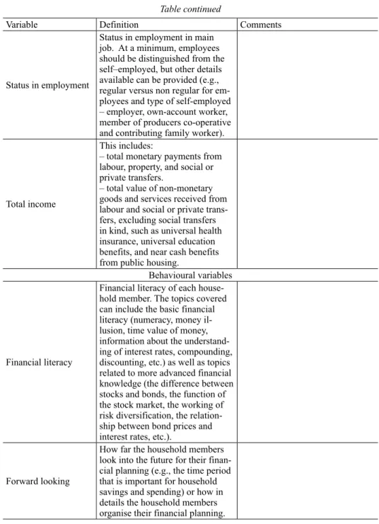
Status in employment
Status in employment in main job. At a minimum, employees should be distinguished from the self–employed, but other details available can be provided (e.g., regular versus non regular for em- ployees and type of self-employed – employer, own-account worker, member of producers co-operative and contributing family worker).
Total income
This includes:
– total monetary payments from labour, property, and social or private transfers.
– total value of non-monetary goods and services received from labour and social or private trans- fers, excluding social transfers in kind, such as universal health insurance, universal education benefits, and near cash benefits from public housing.
Behavioural variables
Financial literacy
Financial literacy of each house- hold member. The topics covered can include the basic financial literacy (numeracy, money il- lusion, time value of money, information about the understand- ing of interest rates, compounding, discounting, etc.) as well as topics related to more advanced financial knowledge (the difference between stocks and bonds, the function of the stock market, the working of risk diversification, the relation- ship between bond prices and interest rates, etc.).
Forward looking
How far the household members look into the future for their finan- cial planning (e.g., the time period that is important for household savings and spending) or how in details the household members organise their financial planning.
Table continued
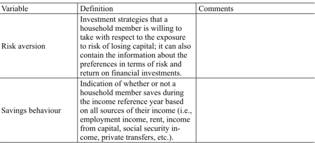
Variable Definition Comments
Risk aversion
Investment strategies that a household member is willing to take with respect to the exposure to risk of losing capital; it can also contain the information about the preferences in terms of risk and return on financial investments.
Savings behaviour
Indication of whether or not a household member saves during the income reference year based on all sources of their income (i.e., employment income, rent, income from capital, social security in- come, private transfers, etc.).
APPENDIX B Model estimates Italy
Table A.1. Summary statistics [1] Prefers
financial invest- ments with very high returns, but with a high risk of losing part of the capital
[2] Prefers financial invest- ments with a good return, but also a fair degree of pro- tection for the invested capital
[3] Prefers financial invest- ments with a fair return, with a good degree of protection for the invested capital
[4] Prefers financial invest- ments with low returns, with no risk of losing the invested capital
Less than 24 (%) 1 22 35 42
25–34 (%) 1 22 36 42
35–44 (%) 1 21 35 43
45–54 (%) 1 22 35 42
55–64 (%) 1 20 35 44
65 and over (%) 1 15 27 58
Gamma 0.11
[1] Male (%) 1 20 34 45
[2] Female (%) 1 19 33 47
Gamma 0.03
[0] None (%) 1 19 30 49
[10] Primary school
(%) 1 16 25 58
[20] Lower secondary
school (%) 1 20 33 47
[31] Vocational second
school (%) 1 20 34 45
[32] Upper secondary
school (%) 1 22 38 39
[51] 3-year university
(%) 1 22 39 38
[52] 5-year university
(%) 1 23 41 34
[60] Postgraduate
qualification (%) 1 22 43 34
Gamma –0.13
Table A.1. continued [1] Prefers
financial invest- ments with very high returns, but with a high risk of losing part of the capital
[2] Prefers financial invest- ments with a good return, but also a fair degree of pro- tection for the invested capital
[3] Prefers financial invest- ments with a fair return, with a good degree of protection for the invested capital
[4] Prefers financial invest- ments with low returns, with no risk of losing the invested capital
[110] Regular employee
(%) 1 21 36 42
[120] Non regular
employee (%) 4 15 23 58
[200] Self-employed
(%) 0 0 100 0
[210] Employer (%) 1 25 37 37
[220] Own-account
workers (%) 1 22 38 39
[240] Contributing fam-
ily workers (%) 0 26 35 39
Gamma –0.044
[1] Agriculture (%) 0 17 32 51
[2] Industry (%) 1 19 31 48
[3] Services (%) 1 22 39 38
Gamma –0.14
Average income, EUR 16952.25 14722.3 14896.33 12655.08 [0] Not living with own
children (%) 1 17 30 52
[1] Living with 1 own
child (%) 1 19 34 46
[2] Living with 2 own
children (%) 1 22 36 41
[3] Living with 3 own
children (%) 0 24 34 42
[4] Living with 4 own
children (%) 2 20 42 37
[5] Living with 5 own
children (%) 0 45 18 36
[6] Living with 6 own
children (%) 0 0 100 0
Gamma –0.12
Table A.1. continued [1] Prefers
financial invest- ments with very high returns, but with a high risk of losing part of the capital
[2] Prefers financial invest- ments with a good return, but also a fair degree of pro- tection for the invested capital
[3] Prefers financial invest- ments with a fair return, with a good degree of protection for the invested capital
[4] Prefers financial invest- ments with low returns, with no risk of losing the invested capital
[11] Does not save:
expenses higher than income (%)
1 15 30 54
[12] Does not save: ex- penses equal to income (%)
1 18 29 52
[20] Saves (%) 1 20 36 44
Gamma –0.11
Average accumulated stock of assets in vol- untary pension account, EUR
468.3417 168.9029 239.0009 101.2987
Quantile of income (%)
1st 1 17 30 52
2nd 1 19 34 46
3rd 1 22 36 41
4th 0 24 34 42
5th 2 20 42 37
If I had to change a job my priority would be : Working in a healthy
safe place (%) 1 18 39 42
A secure job, without the risk of company shutdown or of dis- missal (%)
2 20 37 42
Working in healthy safe place is my priority (1st & 2nd priority if I had to change a job) (%)
1 18 39 42
A secure job, without the risk of company shutdown or of dis- missal (1st & 2nd priority if I had to change a job) (%)
2 20 37 42
Table A.1. continued [1] Prefers
financial invest- ments with very high returns, but with a high risk of losing part of the capital
[2] Prefers financial invest- ments with a good return, but also a fair degree of pro- tection for the invested capital
[3] Prefers financial invest- ments with a fair return, with a good degree of protection for the invested capital
[4] Prefers financial invest- ments with low returns, with no risk of losing the invested capital
Refuse to give up 2%
(patient) (in per cent) 1 24 29 46
Accept to give up 2%
and refuse 5% (in per cent)
1 18 39 41
Accept to give up 5%
and refuse 10% (in per cent)
2 17 43 39
Accept to give 10% and
refuse 20% (in per cent) 0 19 32 49
Accept to give up 20%
(impatient) (in per cent) 2 16 24 57
Gamma 0.09
Having voluntary health
insurance (%) 2 16 44 38
Not having voluntary
health insurance (%) 1 20 32 47
Gamma 0.08
Poor (%) 1 18 26 56
Gamma 0.11
Source: Own study based on LWS data.
Table A.2. Weighted Tobit model with time preference as one of the independent variable.
The dependent variable is the amount accumulated in the voluntary pension account Variable Coefficient
Age –2.512
(39.20)
Female –4,890*
(2,847) 2. Medium level of
education 17,510***
(3,665) 3. Higher level of educa-
tion 23,565***
(5,302) 2. Time preference 2
(preference for the pres- ent)
–3,500
(5,231) 3. Time preference 3 4,647
(4,827) 4. Time preference 4 1,049
(4,239) 5. Time preference 5
(patient) –984.6
(4,146) Correct answer to the
inflation question –4,210**
(2,073)
Personal Income 0.147***
(0.0410)
Constant –58,124***
(11,986)
Observations 9,852
Note: The model was estimated for the entire sample. *** significant at 1% level, ** significant at 5% level,
* significant at 10% level. Standard errors in parentheses.
Source: The model was estimated using Stata software and LWS data.
Table A.3. Weighted Tobit model with risk attitude as one of the independent variable.
The dependent variable is the amount accumulated in the voluntary pension account
Variable Coefficient
Age –1,733***
(167.2)
Female –9,830***
(2,896) 2. Medium level of educa-
tion 23,375***
(3,916) 3. Higher level of education 29,271***
(4,706) 2. Prefers financial invest-
ments with a good return, but also a fair degree of protection for the invested capital
–23,803***
(8,306)
3. Prefers financial invest- ments with a fair return, with a good degree of protection for the invested capital
–15,600*
(7,959)
4. Prefers financial invest- ments with low returns, with no risk of losing the invested capital
–23,911***
(8,119)
Financial literacy –3,275 (3,481) Financial literacy 2 15,762***
(3,424)
Household income 0.358***
(0.0582)
Constant 6,574
(10,798)
Observations 7,721
Note: The model was estimated for the whole sample. *** significant at 1% level, ** significant at 5% level,
* significant at 10% level, Standard errors in parentheses.
Source: The model was estimated using Stata software and LWS data.
UK
Table A.4. Summary statistics Risk tolerant
(1) 2 3 4 Risk averse
(5)
Less than 24 (%) 1 9 23 48 19
25–34 (%) 2 8 20 47 23
35–44 (%) 1 9 18 48 24
45–54 (%) 1 9 16 47 27
55–64 (%) 1 8 13 45 33
65 and over (%) 2 6 14 39 38
Gamma 0.13
[1] Male (%) 2 9 16 44 30
[2] Female (%) 1 7 16 46 30
Gamma 0.034
[110] Married (%) 1 7 14 46 31
[120] In consensual
union (%) 2 9 17 46 25
[210] Never married/
no (%) 2 8 20 45 24
[221] Separated (%) 3 9 19 40 30
[222] Divorced (%) 2 8 17 42 30
[223] Widowed (%) 2 7 16 38 37
[0] Not living with
own children (%) 1 7 15 44 32
[1] Living with 1 own
child (%) 2 8 16 44 30
[2] Living with 2 own
children (%) 1 9 18 48 24
[3] Living with 3 own
children (%) 1 9 18 47 25
[4] Living with more than 4 own children (%)
3 8 21 46 22
Gamma –0.09
[1] Low education
(%) 2 8 20 38 31
[2] Medium (%) 1 7 15 46 30
[3] High education
(%) 1 8 15 47 29
Gamma 0.013
Table A.4. continued Risk tolerant
(1) 2 3 4 Risk averse
(5) [100] Dependent
employed (%) 1 8 16 49 26
[122] Apprentice /
training (%) 0 17 17 28 39
[200] Self-employed
(%) 0 0 0 100 0
[210] Employer (%) 3 8 15 43 32
[220] Own-account
work (%) 1 10 15 45 28
[240] Contributing
family workers (%) 2 4 19 40 36
Gamma 0.01
[1] Agriculture (%) 2 11 17 48 22
[2] Industry (%) 1 9 17 49 24
[3] Services (%) 1 8 15 48 27
Gamma 0.065
[1] Very good health
(%) 1 8 15 45 30
[2] Good health (%) 1 8 15 48 28
[3] Fair (%) 2 8 16 41 33
[4] Bad health (%) 3 8 19 39 31
[5] Very bad health
(%) 5 7 23 33 33
Gamma –0.0049 Average personal
income (GBP) 20,208.42 26,593.36 22,658.01 23,487.67 22,445.58 Average household
income (GBP) 30,716 38,232 34,829 37,531 35,453.35
Average accumulated stock of assets in voluntary pension account (GBP)
4293.068 11289.25 5635.431 4444.046 3786.164
Table A.4. continued Risk tolerant
(1) 2 3 4 Risk averse
(5) [3] Don’t know / no
opinion (%) 6 5 38 33 19
[2] One in five chance to win 10000 (%)
2 12 17 47 23
[1] Guaranteed
payment of 1000 (%) 1 7 15 45 32
Gamma 0.19
[1] £1,000 today (%) 2 7 16 45 30
[2] £1,100 next year
(%) 1 8 14 46 31
[3] Don’t know / no
opinion (%) 7 4 45 22 23
Gamma 0.02
Take a risk to get a good return
[0] Don’t know (%) 8 12 9 38 34
[1] Agree Strongly
(%) 3 9 9 16 62
[2] Agree (%) 1 8 11 56 24
[3] Neither agree nor
disagree (%) 1 3 38 36 22
[4] Disagree (%) 1 12 5 46 36
[5] Disagree strongly
(%) 21 5 3 10 62
Gamma –0.06
Source: Own study based on LWS data.
Table A.5. Weighted Tobit model. The dependent variable is the amount accumulated in voluntary pension account
Variable Coefficient
2. Fair toward risk –28,933***
(7,002)
3. Risk averse –23,064***
(5,673) Avoid the risky gamble –16,346***
(4,154) Wait for differed payment 19,150***
(3,948)
Female –47,770***
(3,792)
Age 1,427***
(157,3) 2. Medium level of education 50,167***
(8,835) 3. High level of education 71,860***
(9,098) 1. Dependent employed,
apprentice / trainee |(ref) 0 (0)
2. Self-employed –870,832
(0)
3. Employer 94,851***
(10,424) 4. Own-account worker 40,785***
(5,107) 5. Contributing family worker –74,255**
(33,831)
2. Industry 9,730
(16,296)
3. Services –13,852
(16,038)
Constant –156,569***
(20,950)
Observations 14,968
Note: The model is estimated for the whole sample, i.e. for the individuals who save and do not save.
Source: The model was estimated using Stata software and LWS data. *** significant at 1% level, ** significant at 5% level, * significant at 10% level. Standard errors in parentheses.
USA
Table A.6. Summary statistics [1] Takes
substantial financial risks expecting to earn substan- tial return
[2] Takes above average financial risks expecting to earn above average return
[3] Takes average financial risks expecting average return
[4] Not will- ing to take any financial risk
Less than 24 (%) 5 20 37 38
25–34 (%) 4 18 38 40
35–44 (%) 6 21 38 35
45–54 (%) 5 20 42 32
55–64 (%) 3 19 46 32
65 and over (%) 3 13 41 43
Gamma 0.02
[1] Male (%) 4 20 43 33
[2] Female (%) 4 18 40 39
Gamma 0.09
[100] Married/in union (%) 3 12 30 55
[110] Married (%) 4 21 46 29
[120] In consensual un (%) 4 15 30 51
[210] Never married/no (%) 4 17 38 40
[220] Formerly married (%) 3 13 28 56
[221] Separated (%) 4 8 32 56
[222] Divorced (%) 4 12 35 50
[223] Widowed (%) 2 7 27 64
Chi2 2.80E+03 Pr 0
[1] Low level of education (%) 2 6 17 75
[2] Medium level of education
(%) 3 13 36 48
[3] High level of education (%) 5 26 50 19
Gamma –0.51
[1] White (include Middle Eastern/Arabian with White);
Caucasian (ref) (%)
4 20 44 33
[2] Black/African-American
(%) 4 12 31 53
Table A.6. continued [1] Takes
substantial financial risks expecting to earn substan- tial return
[2] Takes above average financial risks expecting to earn above average return
[3] Takes average financial risks expecting average return
[4] Not will- ing to take any financial risk
[3] Hispanic/Latino (%) 4 8 22 66
[4] Other: Asian, American Indian/Alaska Native, Native Hawaiian/Pacific Islander (%)
7 16 41 36
Gamma 0.28
[1] Excellent health (%) 5 25 46 23
[2] Good health (%) 3 18 42 36
[3] Fair health (%) 4 10 33 53
[4] Poor health (%) 2 7 26 64
Gamma 0.31
[110] Employed, at work (%) 4 21 43 31
[210] Unemployed (%) 4 12 35 49
[220] Not in labour force (%) 6 20 43 31
[221] Retired, pension (%) 2 10 41 47
[222] In education (%) 7 17 38 38
[223] Homemaker (%) 5 22 41 32
[224] Disabled (%) 2 8 22 68
Gamma 0.19
[100] Dependent employee (%) 4 19 41 36
[200] Self-employed (%) 7 27 49 17
Gamma –0.33
[1] Agriculture (%) 7 18 38 37
[2] Industry (%) 4 18 42 36
[3] Services (%) 5 22 43 30
Gamma –0.1
Average log income 11.1736 11.09101 10.77835 10.08863
Average accumulated stock of assets in voluntary pension account (USD)
170,199.5 211,779.2 122,157.5 110,86.41
Table A.6. continued [1] Takes
substantial financial risks expecting to earn substan- tial return
[2] Takes above average financial risks expecting to earn above average return
[3] Takes average financial risks expecting average return
[4] Not will- ing to take any financial risk
[0] Not living with own chil-
dren (%) 3 17 43 37
[1] Living with 1 own child
(%) 5 17 39 38
[2] Living with 2 own children
(%) 4 24 42 30
[3] Living with 3 own children
(%) 6 26 34 34
[4] Living with 4 own children
(%) 3 16 43 38
[5] Living with 5 own children
(%) 3 17 39 41
[6] Living with 6 own children
(%) 26 11 21 42
[7] Living with 7 own children
(%) 0 0 67 33
Gamma –0.0875
[1] Next few months are the most important for my budget plan (%)
3 10 25 62
[2] Next year is the most im-
portant for my budget plan (%) 4 14 39 43
[3] Next few years are the most important for my budget plan (%)
4 19 41 36
[4] Next 5–10 years are the most important for my budget plan (%)
4 23 50 23
[5] Longer than 10 years are the most important for my budget plan (%)
7 30 47 17
Gamma –0.36
Does not save: usually spend
more than income (%) 9 8 22 61
Gamma 0.33
Table A.6. continued [1] Takes
substantial financial risks expecting to earn substan- tial return
[2] Takes above average financial risks expecting to earn above average return
[3] Takes average financial risks expecting average return
[4] Not will- ing to take any financial risk
Does not save: I spend as much
as my income (%) 4 10 24 63
Gamma 0.46
Saves whatever is left (%) 4 15 40 41
Gamma 0.13
Saves income of one family member and spends the other (%)
4 26 48 23
Gamma –0.21
Spends regular income and
saves the rest (%) 5 29 48 17
Gamma –0.33
Saves regularly by putting
money aside each month (%) 4 25 46 25
Gamma –0.32
Source: Own study based on LWS data.
Table A.7. Weighted Tobit model. The dependent variable is the amount accumulated in voluntary pension account
Variable Coefficient
Age 6,561***
(251.4)
Female –38,726***
(7,234)
2. Medium education 255,307***
(21,462)
3. High education 406,468***
(21,953) 2. Takes above average financial risks
expecting to earn above average return 37,828*
(20,859) 3. Takes average financial risks expecting
average return 6,8117
(19,912) 4. Not willing to take any financial risk –169,256***
(20,385) 2. Next year is the most important for my
budget plan 6,467
(12,340) 3. Next few years is the most important for
my budget plan 24,737**
(10,385) 4. Next 5–10 years is the most important
for my budget plan 43,408***
(10,897) 5. Longer than 10 years is the most impor-
tant for my budget plan 141,847***
(12,426)
Household income 178,096***
(4,953)
2. Black/African-American –78,835***
(11,697)
3. Hispanic/Latino –100,007***
(15,094) 4. Other: Asian, American Indian/Alaska
Native, Native Hawaiian/Pacific Islander –33,818**
(16,364)
Table A.7. continued
Variable Coefficient
Number of children –38,008***
(3,688) 2. I don’t save I spend as much as my
income 36,351
(22,752)
3. I save whatever is left 61,718***
(21,635) 4. Saves income of one family member and
spends the other 52,758
(32,101) 5. Spends regular income and saves the rest 89,598***
(25,811) 6. Saves regularly by putting money aside
each month 93,167***
(21,458)
Constant –2.731e+06***
(63,402)
Observations 29,679
Note: The model is estimated for the whole sample, i.e. for the individuals who save and do not save.
Source: The model was estimated using Stata software and LWS data. *** significant at 1% level, ** significant at 5% level, * significant at 10% level. Standard errors in parentheses.


![Table A.1. Summary statistics [1] Prefers](https://thumb-eu.123doks.com/thumbv2/9dokorg/1323280.106703/20.714.85.620.255.883/table-a-summary-statistics-prefers.webp)
![Table A.1. continued [1] Prefers](https://thumb-eu.123doks.com/thumbv2/9dokorg/1323280.106703/21.714.94.629.159.897/table-a-continued-prefers.webp)
![Table A.1. continued [1] Prefers](https://thumb-eu.123doks.com/thumbv2/9dokorg/1323280.106703/22.714.85.616.156.921/table-a-continued-prefers.webp)
