The assessment of government incentives on savings, Hungary 2006 – 2019
VIVIEN CZECZELI
1, G ABOR KUTASI
1pand ESZTER SZAB O
21Research Institute of Competitiveness and Economy, National University of Public Service, Budapest, Ludovika ter 2, H-1083, Hungary
2Department of World Economy, Corvinus University of Budapest, Hungary
Received: April 4, 2019 • Revised manuscript received: January 30, 2021 • Accepted: March 31, 2021
© 2021 The Author(s)
ABSTRACT
This study analyses the effectiveness of government incentives on household savings in Hungary prior to the Covid pandemic and the ensuing economic turmoil. Time series pertaining to life insurance, voluntary pension savings, and long-term and short-term government bonds are tested in relation to government incentives. The novelty of this study is the test on complex mix of policy incentives and saving funds. The analysis applies the multiple breakpoint test and OLS regression, based on the behavioural life cycle hy- pothesis. The conclusion is that in the analysed time period the government incentives had a significant effect and promoted savings behaviour, with the exception of short-term government bonds.
KEYWORDS
government incentives, household savings, breakpoint test, behavioural life cycle hypothesis, Hungary
JEL CLASSIFICATION INDICES C22, D14, D15, E21
1. INTRODUCTION
In theory, there are several ways in which fiscal policy can have an impact on savings. On the one hand, the government can vary the amount of procurement and the size of financial transfers and, on the other hand, the tax rates can be modified by policy decision makers. If personal taxes are reduced, the disposable income of households will increase and there may be a
pCorresponding author. E-mail: kutasi.gabor@uni-nke.hu
greater scope for savings, depending on households’ propensity to save. Private consumption and private savings are dependent on disposable income, and thus, tax cuts may lead to changes in the use of GDP so that consumption and/or savings will increase. However, this effect is dependent on the marginal propensity to consume.
The question, therefore, is the following: How effective is the economic policy in increasing the multiplier effect? This effect is determined by the marginal propensity to consume and save.
Since tax cuts affect the amount of disposable income available, the response of the private sector to a reduction of tax rates needs to be considered. Without knowing the behaviour of the private sector, it is impossible to estimate the real impact of tax cuts on national income and savings.
Textbook models of macroeconomics describe savings as disposable income less con- sumption. Consumption is defined as a function of need and income. Neo-classical microeco- nomics make calculations assuming that individuals plan with a finite time horizon. In this approach, individuals optimise their consumption and savings for their life expectancy. The risk of declining old-age income is assumed to motivate households to save in their active years.
Our paper tests the effectiveness of government to promote household savings using data on the net financial wealth of households (as a proxy of households’ savings), unit-linked life in- surance, voluntary pension funds and long-term (5-year) and short-term (12-month) govern- ment bond investments. These times series are available in quarterly breakdowns which provide sufficient data for regression analysis. The following specific government incentives are taken into consideration: an increase in the tax credit limit for voluntary pension funds, tax benefits on the employer’s contribution to voluntary pension funds, the termination and reintroduction of tax benefits on unit-linked life insurance, a 5-year interest rate premium on long-term retail government bonds and a 12-month interest rate premium on short-term retail government bonds.
Our hypothesis is that each incentive will cause a breakpoint in the time series and be detectable by OLS regression analysis, which would imply that the incentive is effective.
(Technically the null hypothesis is that there is no effect.) The research aims to reveal whether the government can influence the behaviour of the Hungarian households in financial saving decisions.
2. THEORETICAL BACKGROUND AND EMPIRICAL ANTECEDENT
Kapounek et al. (2016) argued that savings can be influenced by the decisions taken by gov- ernments, the corporate sector and households. According to their study, saving behaviour is also dependent on the social, economic and demographic characteristics of the household sector.
The paper reviews the approach known as thelife-cycle hypothesis(LCH), which was formulated by Modigliani (1966)and Sturm (1983). The life-cycle they described was divided into active and inactive periods. Savings targets are grouped into four categories by the LCH model:
retirement, precautionary reserve, bequest and purchase of tangible assets. The model assumes a steady state economy. According toSturm (1983), the following variables determine the will- ingness of the household sector to save: life expectancy, retirement age, age distribution, family size, average age of employment and skill level. More recently, however, the LCH model has been questioned from the perspective of the behavioural economics concept of household preferences. Diamond – Vartiainen (2007) identified the self-control problems, such as
households’preference for the present-day consumption opportunities compared to saving for the future, and the association of savings with individual desires and related “temptations”, rather than with rational foresight. Prior to this,Laibson (1997)had already established that the utility function for the full lifetime changes with an individual’s age, as does the optimum level of savings. The optimisation of lifetime savings, it seems, is a moving target on a personal level.
All these conclusions led to the development of thebehavioural life-cycle hypothesis(BLCH).
Empirical applications have confirmed that there is a one-way relationship between savings and the improvement of other macroeconomic indicators, such as economic growth, economic development, financial development and disposable income. Moreover, empirical studies employing the BLCH concluded that savings affects inflation and real interest rates. In addition, there is a reverse relationship between savings and foreign trade, capital inflow, political instability and public debt. At the same time, no measurable impact on savings has been found for family status, family size, the level of education of the head of the family or the level of employment.1
The regression analysis of our paper is based on the BLCH theory related toShefrin–Thaler (1988). BLCH is characterised as a critical enrichment of LCH for factors of households’savings.
The BLCH model originates in psychology and replaces the rational choice assumed by earlier models with an effort of self-control which is influenced by internal conflict between rational and emotional aspects, temptation and willpower, in the context of the bounded rationality (Kahneman–Tversky 1979).
Behavioural determinants for the analysis can be identified based on empirical analyses.
Early empirical studies simply used an extended LCH model without calling it BLCH but can be considered the real forerunners of the behavioural approach in saving analysis.Tachibanaki– Shimono (1986) applied an extended LCH model to a cross-sectional panel database of the Japanese employees’savings and used several household characteristics to decompose the factors affecting savings: age, education, wealth, price of house and loan. Wise (1988) analysed the savings and retirement behaviour of the U.S. households with reference to age and marital status. Among the explicitly BLCH empirical studies, Alessie et al. (1995)tested a socio-eco- nomic panel about the savings structure of elderly Dutch households by age cohort, sex, mar- riage/partner status, education level and purpose of saving. Levin (1998) demonstrated the correlation between savings and marginal propensity of consumption (MPC) of income, MPCs of different assets and,finally, liquidity constraints, while determining“how the consumption of individualsat/ or near retirement(authors’ emphasis) vary with changes in different types of financial asset”. Levin concluded that spending is very sensitive to changes in income but is not particularly sensitive to changes in wealth, while liquidity constraints affect consumption based on theirfinancial or psychological transaction costs.
Other studies have tested the significance of the age cohort of individuals and households and investigated why certain elderly households behave in a different way than would be assumed by the rational choice and the life-cycle hypotheses. B€orsch-Supan et al. (2001) examined the ‘German saving puzzle’, namely, why do elderly, the low-income German households accumulate large amounts of savings when they enjoy a generous public pension
1Among others, works ofFidrmuc et al. (2013)andCrespo et al. (2014)are good general examples for the behavioural financial approach to empirical application.
system and health insurance. Similar research was conducted by Chao et al. (2011) on the
‘Chinese saving puzzle’. They established that the LCH cannot explain savings behaviour completely, and therefore, other factors must be examined.Horioka (2010)investigated Japanese dissaving behaviour among the retired and working people with a background of increasing consumption, reduced social benefits and higher taxes. Lee (2013)surveyed the dividend-yield strategies and concluded that the long-run returns of dividend-yield investment strategies are positively driven by changes in the proportion of the older population, which is consistent with the BLCH.Reyers et al. (2015)analysed the South African policy measures dissuading workers from accessing retirement funds when changing jobs. They considered age, reason for leaving job, education level and amount of funds which became statistically significant. Other behav- ioural variables, such as level of salary, value of assets, self-assessed financial situation, marital status, financial literacy, whether they are receiving financial advice or not, time perspective about future and level of impulsivity were not found to be significant factors, which suggests that individuals may behave irrationally and BLCH is not groundless in their case.
The model of overlapping generations is the baseline in the analysis of saving behaviour carried out byDiamond (1965). In this model, long life expectancy is an endogenous factor and the life of each individual is divided into active and inactive periods. Davila –Leroux (2015) investigated how household optimisation prevails between cash and annuity savings.
Several approaches and methods have been proposed in the literature to analyse the behaviour of households in public or private pension and healthcare systems, as well as the investment strategies of different age groups, in order to confirm the validity of LCH–or other factors–in the context of BLCH. The United States and the United Kingdom were the pioneers in supporting retirement savings through incentives built into the tax system. Attanasio et al.
(2004) examined whether the Individual Retirement Account (IRA) introduced in the United States and the Individual Savings Account (ISA) in the United Kingdom and the Tax-Exempt Special Savings Account (TESSA) created new savings, or whether households only transferred their existing savings into financial assets with tax incentives. The conclusion is that only a relatively small proportion of the transferred funds can actually be considered as new savings, so these policies are costly ways to stimulate savings. Poterba et al. (1993) studied the effect of 401(k) plan on private savings, which is a retirement savings plan for the US employers and offers tax advantages. In the 1980s, 401(k) and IRA payments grew steadily. In 1980, the two funds accounted for less than 5% of retirement savings, but this had risen to a ratio of 47% by 1988. The authors concluded that payments to these programs attracted new savings rather than merely redistributing otherfinancial assets.
Sauter et al. (2010)investigated how tax incentives (and bequest motivation) have affected the demand for life insurance in Germany. All-life insurance represents a major proportion of household savings in Germany. Jappelli –Pistaferri (2001) studied how the 1992 tax reform affected the demand for life insurance policies. Their results do not always support the assumption that tax incentives are effective.Courtemanche–He (2009)analysed the effect of tax incentives on the US healthcare sector. Their model is based on the fact that taxpayers may benefit in different ways from different rates. Their regression is focused on differences (dif- ference-in-differences model), in which a data matrix containing households’characteristics is also an influencing factor, beside the tax impact variable.
Turning to Hungary, in the period prior to the 2008 crisis, the level of household savings was very low.Magas (2018) found that financial vulnerability had increased in Hungary by 2008.
Eased lending conditions encouraged households to spend on consumption and to make housing investments with the help of loans. Benczes (2016)described the long march of the Hungarian economy into economic failure and deterioration by the end of thefirst decade of the 2000s. He surveyed the complex economic and institutional processes which led to this situation including the deficiency of household savings and catastrophic indebtedness in foreign currency loans for a certain proportion of mortgage debt contracts. The latter vulnerability was also described byFidrmuc et al. (2013).Elekes –Halmai (2013)concluded that one of the crucial channels for recovery and for the reform of the European growth model has been the increase in private savings, and the Central European countries turned out to be successful early birds in the 2010s in promoting savings beside other structural factors. Meanwhile,Csaba (2011)pondered the role of defunct capital markets, thus extending savings and capitalising to a more general dimension of dispute.
After the crisis, significant changes occurred, and the household savings rate began to rise (Central Bank of Hungary, MNB 2017). First of all, a rise in the value of housing stock contributed to an increase in gross wealth, but the stock of equity and debt securities also expanded (MNB 2018).
3. METHODOLOGY AND DATA
3.1. Methodology of break point test and OLS regression analysis
The current study analyses the government incentives on household savings. Its impact can be in structural breakpoints and correlations. A structural break means that there is a one-time, exogenous effect in the time series that did not originate in the operation of the economy, and thus, is typically an unexpected change in the time series. This can result in temporary, or even permanent lags in the time series, or in a change in the trend. A structural break can be caused by an event which is non-human in origin, such as a natural disaster, but it can also be the result of economic activity, for example the discovery of an oil field or a gold mine. Furthermore, the changes in institutions or to rules can cause break-like shifts in a time series. The introduction of the government incentives examined in the current paper is another of these latter–regulatory– effects. Recognising structural breaks in time series is a key element of econometric analysis because if this effect on the deterministic variables is not identified, regression models will be subject to significant and severe forecasting errors which could compromise the reliability of the model (Hendry – Neale 1991). At the same time, finding and exploring structural breaks provides an opportunity to demonstrate the effectiveness of institutional and regulatory changes that may otherwise be difficult to quantify, and, which actually have a constant value in the long run or which cannot be quantified. (For example, changing a tax rate or extending the range of services.)
Various breakpoint tests can be applied to indicate the structural breaks. In the current paper, the Bai-Perron test (or multiple breakpoint test) is applied. The Bai-Perron test is able to conduct blind searches, since it is not necessary to specify the presumed structural breakpoints in advance. Moreover, the Bai-Perron test is able to uncover multiple breakpoints together in the time series. If the breakpoints are unknown, they can be identified with the Bai-Perron test, thus allowing delayed effects to also be detected. The whole process is based on the unit root test. The results of the unit root test can be influenced by the existence of structural breaks in the time
series. Peron (1989) suggested the possibility that unit root testing may reveal structural breakpoints in time series. He theorized that a structural break results in a permanent shift of the mean of the time series. He composed a standardized test based on the unit-root hypothesis compared against trend-stationary alternatives with the structural breaks caused by global crises.
Bai and Perron (1998)extended the procedure to cases where more than one breakpoint occurs in the modelling. The framework of their proposition containsmnumber of breakpoints in the standard linear regression model, thus m þ1 regimes follow each other over the entire time horizon. They demonstrated that, by searching for the global minimum of the sum of squares of standard deviations, all the breakpoints which were unknowna priorican be effectively iden- tified. The Bai-Perron test is able tofind the most probable location of the breakpoints based on the global minimum and move on toward the next breakpoint step-by-step in a sequential procedure to proceed to the next breakpoint2.
Besides the breakpoint tests, we employ OLS regression. A two-level OLS structure is applied in the first level of which the sensitivity of quarterly net financial wealth of households is tested for the selected ways of saving (voluntary pension fund, life insurance and short- and long-term retail government bonds) and behavioural or life cycle factors. The next level tests the corre- lation of the specific saving items with their determinants. The regression analysis is executed in a backward stepwise method which excludes the insignificant determinants individually, starting with the one with the lowest P-value, and repeating the process of elimination until only sig- nificant variables remain. The purpose of the method is to strengthen the explanatory power of the restricted regression functions. The aim of the regression analysis is to measure the sig- nificant impacts of government incentives. The list of determinants included in the models was affected by the availability of data in the quarterly breakdowns. The following variables are examined:
The first group is the dependent variables which are assumed to be determined directly by the specific government incentives:
■ life insurance reserves–life,
■ pension fund reserves–pension,
■ short-term securities of central government, 12-month held by households, stock–Sbond,
■ long-term securities of central government, 5-year held by households, stock–Lbond.
These are followed by the main and ultimate dependent variable which is the proxy of households’savings. This variable is determined directly by the specific saving items above and only indirectly by the incentives:
2Several versions of the multiple breakpoint test can be run in the econometrics software (EViews). More than one version of sequential and global testing procedures is available. Sequential versions split the time series until a break- point is found. The procedures are repeated until the null-hypothesis (no breakpoint) is rejected or it is no longer possible to cut and reduce the intervals (Bai 1997;Bai–Perron 1998,2003). Global testing globally minimizes the sum- of-squared residuals tofind a breakpoint during the sequential procedure. One version of global testing (global L breaks vs. none) has a predetermined number of breakpoints, in unweighted (UDmax) and weighted (WDmax) versions maximizing the F-statistics. Another global information criteria version minimizes the Schwarz criteria for consistent estimation of breakpoints (Yao 1988;Liu et al. 1997). The breakpoint test methodology demands the null hypothesis to be‘not effective’and the alternative hypothesis to be‘effective’, which is also applied this way in this study (Varpalotai 2006). Nevertheless, the basic assumption is that the following incentives are effective.
■ netfinancial wealth of households (wealth) as the ultimate dependent variable.
The following macroeconomic“textbook”factors of savings were inserted into the model:
■ current account balance–CA,
■ consumer price index–CPI,
■ public debt to GDP ratio–debt,
■ Number of employed persons, seasonally adjusted–empl.
The non-governmental BLCH model determinants are as follows:
■ share of employees with secondary or tertiary education in the total number of employees, calculated from the number of employees by their highest educational qualification–school,
■ personal disposable income of households–PDI,
■ Business Climate Indicator, balance seasonally adjusted–BCI,
■ 1-year yield from residential real estate investment based on–RE_yield,
■ monthly average annualised agreed rate of EUR deposits to households, weighted by the amount of new business–depo-rate.
In the model, the government incentives are represented by the behavioural determinants listed below, the details of which are included inTable 1:
■ interest rate premium on short-term retail government bond–Sbond-prem,
■ interest rate premium on long-term retail government bond–Lbond-prem,
■ tax benefit on unit linked life insurance, dummy–T_BENlife,
■ voluntary pension fund tax credit limit–T_CREDlimit,
■ voluntary pension fund, tax rate on employer’s contribution–T_RATEfunds.
The OLS regression analysis uses the following equations to study the impact of behavioural factors and government incentives, where«is the residual:
wealth¼b0þb1*wealtht−1þb2*lifeþb3*pensionþb4*Sbondþb5*Lbondþb6*CA þb7*CPIþb8*debtþb9*empl þb10*schoolþb11*PDIþb12*BCI
þb13*RE yieldþb14*depo rateþ«; (1)
life¼b0þb1*lifet−1þb2*CAþb3*CPIþb4*debtþb5*emplþb6*schoolþb7*PDI þb8*BCIþb9*RE yieldþb10*depo rateþb11*T_BENlife þ«; (2) pension¼b0þb1*pensiont−1þb2*CAþb3*CPIþb4*debtþb5*emplþb6*school
þb7*PDIþb8*BCIþb9*RE yealdþb10*depo rateþb11*T_CREDlimit
þb12*T_RATEfundsþ«; (3)
Lbond¼b0þb1*Lbondt−1þb2*CAþb3*CPIþb4*debtþb5*emplþb6*schoolþb7PDI þb8*BCIþb9*RE yieldþb10*depo rateþb11*Lbond premþ«;
(4) Sbond¼b0þb1*Sbondt−1þb2*CAþb3*CPIþb4*debtþb5*emplþb6*school
þb7PDIþb8*BCIþb9*RE yieldþb10*depo rateþb11*Sbond premþ«: (5)
3.2. Quality of data
There are various measures through which the government can increase the level of household savings. Examining the net financial assets of households reveals the general trends, and con- clusions can be drawn on the effectiveness of targeted incentives based on the insurance sector, retail government securities and fundraisers’data series.
To obtain a higher number of observations (N554), only those variables are included in the database which are available in a quarterly breakdown (Table 2). The deposit stocks of housing savings funds and voluntary healthcare funds are not included in the analysis due to the lack of quarterly data. The availability of behavioural data is also limited. Consequently, the sample starts in 2006Q1 and runs until 2019Q2. The breakpoint tests are conducted independently in Table 1. Government incentives
Variables Incentive Time of introduction/termination
Voluntary pension fund tax credit limit
Increase of tax credit limit (from 100 thousand HUF up to 150
thousand HUF) (T-CREDlimit)
2014Q1
Voluntary pension fund tax rate on employers' contribution, %
Introduction of tax benefit on pension insurance (T-RATEfunds)
2006Q1–25 2011Q1–19.04 2012Q1–30.94 2016Q1–34.51 2017Q1–43.66 2018Q1–40.71 2019Q3–38.35 Fee reserves of life insurance Termination of tax benefit on unit
linked life insurance (T-BENlife)
No benefit:
2010Q1–2013Q4 Short-term government bonds 12-month interest rate premium
(SGBond-prem)
Special premium since 2015Q1 Calculation: Current rate–interest
rate base Long-term government bonds 5-year interest rate premium
(LGBond-prem)
Special premium since 2015Q1 Calculation: Current rate–interest
rate base
Source: Authors' collection, based on the data of the Hungarian Central Statistical Office (HCSO).
Note: Interest rate base: Change of consumer prices in the previous month, if negative, then the base is 0%.
order to cover a longer period of time. The length of the time periods is determined by the availability of data (Table 3).3
4. RESULTS
4.1. Breakpoint tests
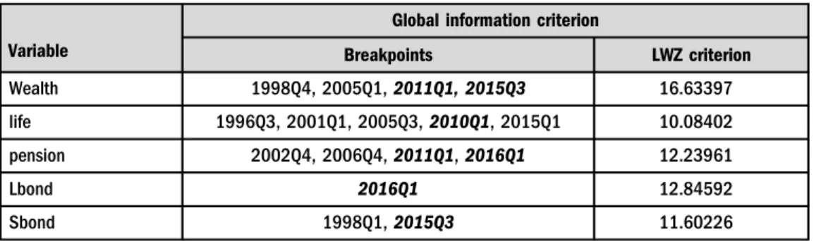
In the multiple Bai-Perron test, a global information criterion version is applied which is based on the LWZ criterion (Liu et al. 1997). The results are summarised inTable 4 indicating the breakpoints that may correspond to the effects of government incentives. It should be noted that the current breakpoint test is a preliminary exploration of the likely efficiency of government incentives anticipating the OLS regression results.
According to the multiple breakpoint test results, it can be established that for voluntary pension funds, 2011Q1 and 2016Q1 are consonant with the dates of changes in the tax policy.
However, this is counterintuitive, as there is a large drop in savings in spite of the lowered tax rate in 2011, which is a cyclical effect rather than the impact of the policy action. This can be observed inFig. 1. The tax benefit on life insurance was terminated in 2010Q1 and was reintroduced in 2014Q1. The breakpoint test appears to indicate that 2010Q1 is a significant break, but the cyclical effect of the globalfinancial crisis cannot be excluded here. As regards the breakpoints related to the extra interest rate premia introduced in 2015Q1 on the short- and long-term government bonds, it is reasonable to assume that households needed time to adjust their portfolios, so the breaks in 2015Q3 for the short-term bonds and in 2016Q1 for the long-term bonds may indicate lagged effects of these measures. This needs to be confirmed by regression analysis, however. Finally, the netfinancial wealth of households mirrors the drop in 2011Q1 and the upturn in 2015Q3, which may confirm the assumption that these are cyclical impacts rather than policy effects.
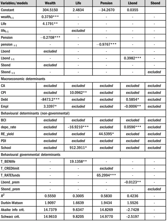
4.2. Regression
Based on the results presented inTable 5on the netfinancial wealth of households it can be noted that life insurance savings and voluntary pension funds have the most significant Table 2.Data availability onfinancial assets of households
Variables Time horizon Unit Frequency
Netfinancial wealth of households (wealth) 1989Q4–2019Q2 bn HUF Quarterly Fee reserves of life insurance (life) 1989Q4–2019Q2 bn HUF Quarterly Fee reserves of pension funds (pension) 1994Q4–2019Q2 bn HUF Quarterly Short-term government bonds (Sbond) 1989Q4–2019Q2 bn HUF Quarterly Long-term government bonds (Lbond) 1991Q4–2019Q2 bn HUF Quarterly Source: MNB.
3The stationarity of the time series is examined with augmented Dickey–Fuller tests. All of the dependent variables and determinants have to be differentiated (seeAppendix).
coefficients. This means that any significant government incentives also affect the wealth in- dicator through the pension fund or life insurance components. The two government bond savings with different maturities are excluded from the determinants of the ultimate aggregate savings (which is substituted by the households’ net financial wealth). It can therefore be concluded that the exclusive retail interest rate premium (as a government incentive) does not influence the overall netfinancial wealth of households through the government bond market.
In addition to the behavioural determinants examined in the current analysis, macroeconomic factors are significant, with the public debt to GDP having a powerful negative and significant impact at 1% significance level, while the employment coefficient has a positive effect of 10%.
Based on the current analysis, the impact of behavioural factors cannot be confirmed. The cyclical component (t–1) is significant and positive, which confirms the assumption mentioned above, in relation to the breakpoint tests, that the introduction of the incentives has had a lagged effect on the quarterly data.
For investigating the four ways of saving, the regression method is found unproductive when applied to data on short-term government bonds since all of the potential determinants are excluded Table 3. Descriptive statistics, 2006Q1–2019Q2
Variables Mean Max Min
Std.
Dev. Source Unit
BCI –0,50 16 –34.7 9.84 European Commission index
CA –3.55 542.37 –625.9 300.32 MNB bn HUF
CPI 3.36 8.6 –1.06 2.49 FRED %
Debt 0.75 0.84 0.64 0.06 AKK % to GDP
depo_rate 4.16 10.60 0.26 3.15 MNB %
empl 4033.13 4515.55 3718.2 271.4 HCSO th person
RE_yield 4.92 17.05 –9.26 8.58 MNB %
Lbond 909.88 3767.61 248.53 823.26 MNB bn HUF
Lbond_prem 2.15 9.56 –1.93 2.34 Author's calculation bn HUF
life 1646.24 2023.53 1081.62 233.01 MNB bn HUF
PDI 4499.39 6544.1 3365.33 801.44 Author's calculation based on HCSO and MNB
bn HUF
pension 2029.96 4062.64 1151.09 822.8 MNB bn HUF
S_bond 1325.18 3130.88 332.14 966.9 MNB bn HUF
School 0.59 0.61 0.55 0.02 HCSO %
Sbond_prem 1.11 7.90 –3.49 2.41 Author's calculation %
T_CREDlimit 1.20 1.50 1.00 0.25 Netjogtar th HUF
T_RATEfunds 30.15 43.66 19.04 6.88 Netjogtar %
Wealth 26330.91 47885.45 15210.62 9919.78 MNB bn HUF
together with the retail interest rate premium. This may be logical behaviour in the short-term, if short-term assets are considered to be a channel for the excessive liquidity of the households, and no other factor matters, but merely an opportunity to invest money in a liquid and risk-free option. The question of the validity of this assumption is beyond the scope of the current analysis. What can be established is that regression analysis does not confirm the breakpoint test results.
Life insurance savings resulted in a positive coefficient for the existence of a tax benefit dummy as a government incentive at a 5% significance level. Moreover, two behavioural Table 4.Breakpoint test, Global information criterion version
Variable
Global information criterion
Breakpoints LWZ criterion
Wealth 1998Q4, 2005Q1,2011Q1, 2015Q3 16.63397
life 1996Q3, 2001Q1, 2005Q3,2010Q1, 2015Q1 10.08402
pension 2002Q4, 2006Q4,2011Q1,2016Q1 12.23961
Lbond 2016Q1 12.84592
Sbond 1998Q1,2015Q3 11.60226
Note: Relevant breakpoints indicated with bold and italic.
Source: Authors' calculation.
Source: MNB.
0 10,000 20,000 30,000 40,000 50,000 60,000
0 1000 2000 3000 4000 5000 6000
2006Q1 2006Q4 2007Q3 2008Q2 2009Q1 2009Q4 2010Q3 2011Q2 2012Q1 2012Q4 2013Q3 2014Q2 2015Q1 2015Q4 2016Q3 2017Q2 2018Q1 2018Q4 2019Q3
life pension Sbond Lbond wealth (right scale)
Fig. 1.Time series of households' savings, 2006Q1 –2019Q3, billion HUF
Table 5. Results of regression models
Variables/models Wealth Life Pension Lbond Sbond
Constant 304.5150 2.4834 34.2670 0.0355
wealtht-1 0.3750*** - - - -
Life 4.1791** - - - -
lifet-1 - excluded - - -
Pension 0.2708*** - - - -
pensiont-1 - - 0.9767*** - -
Lbond excluded - - - -
Lbondt-1 - - - 0.3982*** -
Sbond excluded - - - -
Sbondt-1 - - - - excluded
Macroeconomic determinants
CA excluded excluded excluded excluded excluded
CPI excluded 10.0962** excluded excluded excluded
Debt –8473.2*** excluded excluded 0.5854* excluded
Empl 3.3397* excluded excluded –0.0006** excluded
Behavioural determinants (non-governmental)
BCI excluded excluded excluded excluded excluded
depo_rate excluded –16.9210*** excluded 0.0596*** excluded
RE_yield excluded excluded 44.5395* excluded excluded
PDI excluded excluded excluded excluded excluded
School excluded 912.3911* excluded excluded excluded
Behavioural governmental determinants
T_BENlife - 19.1358** - - -
T_CREDlimit - - excluded - -
T_RATEfunds - - 65.2994*** - -
Lbond_prem - - - –0.0123** -
Sbond_prem - - - - excluded
R2 0.5550 0.3005 0.5830 0.4236 -
Durbin-Watson 1.9097 1.6639 1.9434 1.5526 -
Akaike info crit. 14.7379 9.6347 14.8269 –2.7428 -
Schwarz crit. 14.9610 9.8205 14.9770 –2.5197 -
(continued)
determinants are proved to be statistically significant, the euro deposit rate (depo_rate) with negative sign–which means that a higher deposit rate diverts savings from life insurance,–and higher qualification (school) with positive sign. Finally, higher inflation results in higher life insurance funds at 5% significance.
The effectiveness of one of the government incentives to make contributions to a voluntary pension fund is also verified. The tax rate on employers’contribution has a powerful positive effect with a significance of 1%, which means that the tax incentive has made a notable contribution to achieving the economic policy objective. At the same time, however, raising the tax credit limit on pension savings (T_CREDlimit) does not have a significant influence and is thus excluded from the list of explanatory variables. Apart from these model determinants, only the real estate yield (RE_yield) indicates a significant effect with a positive sign.
Concerning savings in retail long-term government bonds, the exclusive rate premium is proved to be significant at a 5% level with a negative sign. Furthermore, the euro deposit rate and the public debt are significant with positive signs, while the number of persons in employment is significant with a negative sign.
The backward stepwise OLS regression methodology produces the following restricted equa- tions from (6) to (9) for the savings variables of wealth, life, pension and Lbond. The analysis excludes all of the possible determinants with regard to short-term government bonds.
wealth¼304:515þ0;375*wealtht−1þ4:1791*life 0:2708*pension8473:2*debt
þ3:3397*empl; (6)
life¼2:4834þ10:0962*CPIþ912:3911*schoolþ19:1358*T_BENlife; (7) pension¼−34:2670:9767*pensiont−1þ44:5395*RE yealdþ65:2994*T_RATEfunds; (8) Lbond¼0:0355þ0:3982*Lbondt−1þ0:5854*debt0:0006*emplþ0:0596*depo rate
0:0123*Lbond prem: (9)
5. DISCUSSION AND CONCLUSION
We analysed the effectiveness and impact of various Hungarian government incentives on households’ savings. The hypothesis was that each incentive would cause a breakpoint in the time series and prove to be significant in the OLS regression analysis, allowing conclusions to be Table 5.Continued
Variables/models Wealth Life Pension Lbond Sbond
Hannan-Quinn cr. 14.8237 9.7061 14.8845 –2.6570 -
No. of observ. 53 53 52 53 53
Source:Authors' calculation.
Note:Significance: *** at 1%, ** at 5%, * at 10% level.
drawn as to their effectiveness. The research question was whether the government is able to influence the behaviour of Hungarian households when takingfinancial saving decisions.
The overall level of savings of domestic households (net financial wealth of households) as well as the level of some specific types of savings (unit linked life insurance, voluntary pension funds and long-term (5-year) and short-term (12-month) retail government bonds) are tested to determine the impact of related policy incentives (an increase in the tax credit limit of voluntary pension funds, tax benefits for employer’s contributions to voluntary pension funds, the termination and subsequent reintroduction of tax benefits on unit-linked life insurance, a 5-year interest rate premium on long-term retail government bonds and a 12-month interest rate premium on short-term retail government bonds).
The analysis was based on the BLCH model introduced by Shefrin – Thaler (1988). The methodology included both a Bai-Perron multiple breakpoint test and an OLS regression. The double methodology strengthened the robustness of the analysis. The OLS regression confirmed the significance of the termination and reintroduction of tax benefits for unit linked life in- surance, which was clearly reinforced by the results of the breakpoint test regarding the termination. The OLS regression also indicated the significance of changes to the tax rate on employers’contributions to voluntary pension funds, the impact of which was also definitively confirmed by the breakpoint test. Raising the tax credit limit on pension funds was not found to be significant, however. Thefindings about government bond premiums were also mixed. While the long-term interest rate premium proved to be significant, the short-term bonds did not. The breakpoint test results for bond premia can be regarded as an indicator of a lagged effect.
The results are closely concordant with the previous studies referred to in the literature review, which confirmed the significant impact of government incentives (e.g., Hosszu – Dancsik 2018). In comparison, the current novelty is the test on complex mix of incentives and funds which exceeds the empirical literature existed before. The test demonstrated the possibility of herding the households’savings with a mix of government incentives.
ACKNOWLEDGEMENT
This research was supported by MKB Bank and University of Public Service. An early version of this paper was presented at the Conference entitled“EU 2.0: Is Demography Destiny? Savings, Investments and Current Account Dynamics in the EU”, held at Mendel University, Brno (CZ), May 17–18, 2018. Helpful comments by the participants of this conference, from the MKB Bank and by the anonymous referees of this journal are gratefully acknowledged.
REFERENCES
Alessie, R.–Lusardi, A.–Kapteyn, A. (1995): Saving and Wealth Holdings of the Elderly.Ricerche Eco- nomiche, 49(3): 293–314.
Attanasio, O. P.–Banks, J.–Wakefield, M. (2004): Effectiveness of Tax Incentives to Boost (Retirement) Saving: Theoretical Motivation and Empirical Evidence. IFS Working Papers, No. 04/33. London, Institute for Fiscal Studies.
Bai, J. (1997): Estimating Multiple Breaks One at a Time.Econometric Theory, 13(3): 315–352.
Bai, J. – Perron, P. (1998): Estimating and Testing Linear Models with Multiple Structural Changes.
Econometrica, 66(1): 47–78.
Bai, J.–Perron, P. (2003): Computation and Analysis of Multiple Structural Change Models.Journal of Applied Econometrics, 18(1): 1–22.
Benczes, I. (2016): From Goulash Communism to Goulash Populism: The Unwanted Legacy of Reform Socialism.Post-Communist Economies, 28(2): 146–166.
Borsch-Supan, A.–Reil-Held, A.–Rodepeter, R.–Schnabel, R.–Winter, J. (2001): The German Savings Puzzle.Research in Economics, 55(1): 15–38.
Chao, C. C.–Laffargue, J. P.–Yu, E. (2011): The Chinese Saving Puzzle and the Life-Cycle Hypothesis: A Revaluation.China Economic Review, 22(1): 108–120.
Csaba, L. (2011): Financial Institutions in Transition: The Long View.Post-Communist Economies, 23(1):
1–13.
Courtemanche, C.–He, D. (2009): Tax Incentives and the Decision to Purchase Long-Term Care In- surance.Journal of Public Economics, 93(2): 296–310.
Crespo Cuaresma, J.–Fidrmuc, J.–Hake, M. (2014): Demand and Supply Drivers of Foreign Currency Loans in CEECs: A Meta-Analysis.Economic Systems, 38(1): 26–42.
Davila, J.–Leroux, M. L. (2015): Efficiency in Overlapping Generations Economies with Longevity Choices and Fair Annuities.Journal of Macroeconomics, 45(C): 363–383.
Diamond, P. A. (1965): National Debt in a Neoclassical Growth Model.American Economic Review, 55(5):
1126–1150.
Diamond, P.–Vartiainen, H. (2007):Behavioral Economics and its Applications. Princeton, NJ: Princeton University Press.
Elekes, A.– Halmai, P. (2013): Growth Model of the New Member States: Challenges and Prospects.
Intereconomics: Review of European Economic Policy, 48(2): 124–130.
Fidrmuc, J.–Hake, M.–Stix, H. (2013): Households’Foreign Currency Borrowing in Central and Eastern Europe.Journal of Banking&Finance, 37(6): 1880–1897.
Horioka, C. (2010): The (Dis)Saving Behavior of the Aged in Japan. Japan and the World Economy (Elsevier), 22(3): 151–158.
Hosszu, Zs.–Dancsik, B. (2018): Measuring Bank Efficiency and Market Power in the Household and Corporate Credit Markets Considering Credit Risks.Acta Oeconomica, 68(2): 175–207.
Jappelli, T.–Pistaferri, L. (2001): Tax Incentives and the Demand for Life Insurance: Evidence from Italy.
Naples: Centre for Studies in Economics and Finance (CSEF), University Naples, Working Paper, No. 52.
Kahneman, D.–Tversky, A. (1979): Prospect Theory: An Analysis of Decision Under Risk.Econometrica, 47(2): 263–291.
Kapounek, S.–Korab, P.–Deltuvaite, V. (2016): (Ir)Rational Households’Saving Behavior? An Empirical Investigation.Procedia Economics and Finance, 39(1): 625–633.
Laibson, D. (1997): Golden Eggs and Hyperbolic Discounting.Quarterly Journal of Economics, 112(2): 443–
477.
Lee, K. (2013): Demographics and the Long-Horizon Returns of Dividend-Yield Strategies.The Quarterly Review of Economics and Finance, 53(2): 202–218.
Levin, L. (1998): Are Assets Fungible? Testing the Behavioral Theory of Life-Cycle Savings. Journal of Economic Behavior&Organization, 36(1): 59–83.
Liu, J.–Wu, S.–Zidek, J. (1997): On Segmented Multivariate Regression.Statistica Sinica, 497–525.
Magas, I. (2018): Financial Adjustment in Small, Open Economies in Light of the “Impossible Trinity”
Trilemma.Financial and Economic Review, 17(1): 5–33.
Modigliani, F. (1966): The Life Cycle Hypothesis of Saving, the Demand for Wealth and the Supply of Capital.Social Research, 33(2): 160–217.
National Bank of Hungary (2017): Insurance, Funds and Capital Market Risk Report.Https://Www.Mnb.
Hu/En/Publications/Reports/Insurance-Funds-And-Capital-Market-Risk-Report.
National Bank of Hungary (2018): Insurance, Funds and Capital Market Risk Report.Https://Www.Mnb.
Hu/En/Publications/Reports/Insurance-Funds-And-Capital-Market-Risk-Report.
Perron, P. (1989): The Great Crash, the Oil Price Shock and the Unit Root Hypothesis.Econometrica, 57:
1361–1401.
Poterba, J. M.–Venti, S. F.–Wise, D. A. (1993): Do 401(K) Contributions Crowd Out Other Personal Saving?NBER Working Paper, No. 4391.
Reyers, M.–Schalkwyk, C.–Gouws, D. (2015): Rational and Behavioural Predictors of Pre-Retirement Cash-Outs.Journal of Economic Psychology, 47C: 23–33.
Sauter, N.–Walliser, J.–Winter, J. (2010): Tax Incentives, Bequest Motives, and the Demand for Life Insurance: Evidence from Two Natural Experiments in Germany. Cesifo Working Paper, No. 3040, Munich.
Sherfin, H. M.–Thaler, R. H. (1988): The Behavioral Life-Cycle Hypothesis.Economic Inquiry, 26(4): 609–
643.
Sturm, P. H. (1983): Determinants of Saving: Theory and Evidence.OECD Economic Studies, 1(1): 147–
196.
Tachibanaki, T.–Shimono, K. (1986): Saving and the Life-Cycle: A Cohort Analysis. Journal of Public Economics, 31(1): 1–24.
Varpalotai, V. (2006): Id}oben valtozo valos rend}u eltolases becslese (Time-Varying Carrier Frequency Offset and Estimation).Statisztikai Szemle, 84(10–11): 966–995.
Wise, D. A. (1988): Saving for Retirement: The U.S. Case. Journal of the Japanese and International Economies, 2(4): 385–416.
Yao, Y. C. (1988): Estimating the Number of Change-Points via Schwarz’Criterion.Statistics&Probability Letters, 6(3): 181–189.
APPENDIX
Results of ADF tests
Variables
Level First diff. Second diff.
T-stat P-value T-stat P-value T-stat P-value
BCI –1.9853 0.2923 –6.1785 0.0000
CA –2.1142 0.24 –6.9738 0.0000
CPI –2.181 0.2154 –4.7415 0.0003
(continued)
Open Access. This is an open-access article distributed under the terms of the Creative Commons Attribution 4.0 International License (https://creativecommons.org/licenses/by/4.0/), which permits unrestricted use, distribution, and reproduction in any medium, provided the original author and source are credited, a link to the CC License is provided, and changes–if any–are indicated. (SID_1)
Continued
Variables
Level First diff. Second diff.
T-stat P-value T-stat P-value T-stat P-value
debt –1.7385 0.4066 –7.9555 0.0000
depo_rate –0.4738 0.8875 –2.9206 0.0508 –5.1671 0.0001
empl 1.427 0.9989 –2.0122 0.2809 –9.6751 0.0000
RE_yield –0.9719 0.7567 –5.0612 0.0001
Lbond 3.5547 1.0000 3.9688 1.0000 –0.9129 0.7759
Lbond_prem –2.1606 0.2227 –6.2877 0.0000
life –2.0868 0.2506 –5.1001 0.0001
PDI 6.6867 1.0000 –2.1564 0.2244 –6.7581 0.0000
pension –1.8463 0.3547 –6.96 0.0000
Sbond –1.7 0.425 –1.6513 0.4497 –6.7356 0.0000
school –2.1554 0.2247 –2.8289 0.0613 –13.394 0.0000
Sbond_prem –2.5855 0.1022 –6.1295 0.0000
T_RATEfunds –1.0794 0.7178 –7.2952 0.0000 T_CREDlimit –0.8455 0.7979 –7.3484 0.0000
wealth 6.7382 1.0000 –4.0215 0.0027
Source:Authors' calculation.
Note: Null hypothesis: Variable has a unit root.