2019. május 24.

AZ ELMÉLET ÉS A GYAKORLAT TALÁLKOZÁSA A TÉRINFORMATIKÁBAN

X.

THEORY MEETS PRACTICE IN GIS

Szerkesztette:

Molnár Vanda Éva Technikai szerkesztők:

Kovács Gergő, Nagy Bálint, Szabó Loránd, Szalóki Annamária, Szopos Noémi Mária

Lektorálták:

Dr. Négyesi Gábor, Dr. Tóth Csaba Albert, Dr. Túri Zoltán Krisztián ISBN 978-963-318-054-9

A kötet a 2019. május 23–24. között Debrecenben megrendezett Térinformatikai Konferencia és Szakkiállítás előadásait tartalmazza.

A közlemények tartalmáért a szerzők a felelősek.

A konferenciát szervezte:

A Debreceni Egyetem Földtudományi Intézete, az MTA Természetföldrajzi Tudományos Bizottság Geoinformatika Albizottsága, az MTA DAB Földtudományi Bizottsága, a Magyar Földrajzi Társaság, a MAGISZ, a HUNAGI

és az eKÖZIG ZRT.

Debrecen Egyetemi Kiadó Debrecen University Press

Készült

Kapitális Nyomdaipari Kft.

Felelős vezető: ifj. Kapusi József Debrecen

2019

Tartalomjegyzék

Program 7

Előadások

Mohd Aaqib Lone – Zsolt Toth: Distance Estimation In IndoorGML Maps 9 Abriha Dávid – Banka Fruzsina – Szabó Szilárd: Random Forest

osztályozó algoritmus pontosságának vizsgálata tetőfedő anyagok

azonosításában multispektrális adatokkal 19

Malak Alasli: Concordance of Maghrebian place names in the Hungarian

school atlases 25

Ashraf ALDabbas – Zoltán Gál: Getting Facts about Interplanetary

Mission of Cassini-Huygens Spacecraft 27

Árvai László: Beltéri navigációs rendszer fejlesztése nyílt forrású alapokon 35 Árvai Mátyás – Deák Márton – Mészáros János: Eróziós térszínek drónos

vizsgálata 41

Bagdi Zsolt: Repülőterek biztonságtechnikai felmérése geoinformatikai

módszerekkel 43

Bakó Gábor – Répás Zoltán – Lehoczky Máté: A Légi Térképészeti és Távérzékelési Egyesület ajánlása a légi távérzékeléssel gyűjtött

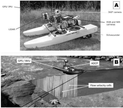
téradatok geometriai pontosságának elemzéséhez 49 Bertalan László – Nagy Bálint – Szopos Noémi Mária – Anette Eltner –

Hannes Sardemann – David Mader: Medertopográfiai és hidrometriai vizsgálatok a Sajó mentén pilóta nélküli vízi- és

légijárművekkel 55

Birinyi Edina – Friedl Zoltán – Hubik Irén – Kristóf Dániel – Nádor Gizella – Rotterné Kulcsár Anikó – Pacskó Vivien – Mikus Gábor:

Felhőalapú adatfeldolgozás távérzékelési alkalmazásokban 61 Biró Csilla Karina – Kubány Csongor: Épület állomány aktualizálása

speciális számításokat igénylő projekt nagy adatmennyiséget

tartalmazó alaptérképéhez – Esettanulmány 67

Burai Péter – Gaál Márta – Molnár András – Tomor Tamás –

Bekő László: Halastavak vizsgálata távérzékelési módszerekkel 71 Czimber Kornél – Burai Péter – Kovács Zoltán – Gerencsér

Albert: Erdőleltározás légi lézeres letapogatással és közel

fotogrammetriával – Első tesztek eredményei 77

Göttlinger István R. – Schüszler Péter: Síkvidéki vízrendezés tervezési

alapjainak megújítása a térinformatika eszközeivel 83 Gudmann András – Mucsi László: Döntési fa és véletlen erdő osztályozási

módszerekkel készített felszínborítási térképek pontosságának

összehasonlító elemzése 91

Gyenizse Péter – Pap Norbert – Kitanics Máté – Morva Tamás: A mohácsi csata helyszínének pontosítását célzó beláthatósági vizsgálatok

eredményei 101

Gyuris Péter – Sápi Dávid – Kovács Ferenc: Bioenergetikai szempontú

felmérések marginális, művelés alól kivont területeken 109 Hegedűs László Dávid: Az átszállásmentes közlekedés vizsgálata Debrecenben 117 Karancsi Gergő – Baranyi Imre – Lázár Vilmos – Balla Dániel: Talajban

tárolt szennyezőanyag mennyiségének becslése RockWorks

program segítségével 123

Kern Anikó – Dobor Laura – Horváth Ferenc – Hollós Roland – Márta Gergely – Barcza Zoltán: FORESEE: egy publikus

meteorológiai adatbázis a Kárpát-medence tágabb térségére 131 Kinárov Krisztián – Túri Zoltán Krisztián – Gönczy Sándor: Űrfelvétel-

alapú változásvizsgálatok a Beregszászi-dombságon 139 Kiss Kinga – Czigány Szabolcs – Valkay Alexandra Ilona –

Marcin Słowik – Remigiusz Tritt – Adam Marciniak – Balogh Richárd – Dezső József – Lóczy Dénes – Halmai Ákos – Pirkhoffer Ervin: A magyarországi kisvízfolyások paleomeder-

vizsgálatának modellezése 147

László Kiss: Analysis and visualization of the Heating Degree Days in the

Benelux states 153

Koós Sándor – Laborczi Annamária – Szatmári Gábor – Pirkó Béla – Csathó Péter – Szabó Anita – Fodor Nándor – Pásztor László: A

nitrát érzékeny területek nitrogén forgalmának térbeli modellezése 159 Kovács Gergő – Szabó Gergely: A beépítettség kimutathatósága digitális

felszínmodelleken, Debrecen példáján 161

Kovalcsik Tamás: Társadalmi és politikai términtázatok aggregációs

lehetőségei mikroléptéken, Budapest példáján 167 Laborczi Annamária – Szabó Brigitta – Szatmári Gábor – András Makó –

Zsófia Bakacsi – Pásztor László: Talaj-vízgazdálkodási kategóriák térképezése digitális hidrofizikai talajtulajdonság térképek és

archív talajtérképek alapján, adatbányászati módszerekkel 175 Mészáros János – Nemerkényi Zsombor – Nagy Balázs: UAV felmérések

magashegységi környezetben – Ojos del Salado, Chile 177 Mészáros Márk: A közúti járműgyártás és a kapcsolódó iparágak súlypont

változásainak vizsgálata Magyarországon 179

Mihalik József: A HM Zrínyi Térképészeti és Kommunikációs Szolgáltató

Közhasznú Nonprofit Korlátolt Felelősségű Társaság Légifényképtára 187 Dragan D. Milošević – Jan Geletič – Stevan M. Savić – Michal Lehnert:

Intra-urban analysis of land surface temperatures in the City of

Novi Sad (Serbia) 193

Molnár Vanda Éva – Simon Edina – Szabó Szilárd: Fafajok osztályozása

multispektrális felvételek alapján debreceni mintaterületen 201 Nagy Bálint – Szopos Noémi Mária: Hidrológiai modellekben

bekövetkező változások eltérő felbontású digitális

domborzatmodellek alkalmazása esetén 205

Nagy Géza: A CUBE, mint átfogó térinformatikai megoldás a Stonex-től 211 Neuberger Hajnalka – Juhász Attila – Krausz Nikol – Potó Vivien –

Barsi Árpád: Voxel alapú környezetmodell lézerszkennelés alapján 215 Daniel O. Nyangweso – Mátyás Gede: Integration of Toponyms Mobile

data Collection in PostgreSQL Database 225

Orgoványi Péter – Salamon Endre: Térinformatika alkalmazása

víziközműves szakmai tárgyak oktatása során 233

Papp István: A határ menti területek lehatárolása térinformatikai módszerekkel 239 Pásztor László – Laborczi Annamária – Szatmári Gábor: Standardizált vs.

specifikus digitális talajtérképek: hajtóerők, kölcsönhatások,

lehetőségek 247

Pődör Andrea – Bosföldi Dorina – Katonáné Gombás Katalin: Zajérzet

mérése Székesfehérváron és Szombathelyen 249

Andrea Procházková – Tomáš Mikita: Utilization of the hand-held mobile

laser scanning in forest inventory 257

Schlosser Aletta Dóra – Szabó Gergely – Varga Zsolt – Enyedi Péter:

Épületobjektumok detektálása fotogrammetriai pontfelhő

alkalmazásával debreceni mintaterületen 259

Schneck Tamás – Telbisz Tamás – Zsuffa István: Csapadék-interpoláció digitális terepmodell és többváltozós regressziószámítás

felhasználásával magyarországi hegységi mintaterületekre 263 Stenzel Sándor: Korszerű 3D-technológiák az UVATERV Zrt.-nél 271 Sütő László – Balogh Szabolcs – Rózsa Péter: Antropogén bolygatottság a

Borsodi-medencében 275

Szabó Gergely – Schlosser Aletta Dóra: Fotogrammetriai felszínmodell

pontosságvizsgálata RTK-UAV alkalmazásával 281

Szabó Loránd – Szabó Szilárd: Hosszútávú vegetációterjedés-monitoring

a Tisza-tó területén spektrális indexek alkalmazásával 287 Szabó Zsuzsanna – Szabó József – Tomor Tamás – Baranyai Edina –

Prokisch József – Szabó Szilárd: Az ártér geomorfológiájának

szerepe a nehézfémek mintázatában Sajó menti mintaterületen 293 Szabó Zsuzsanna – Szabó József – Tomor Tamás – Baranyai Edina –

Prokisch József – Szabó Szilárd: Övzátonyok és sarlólaposok

nehézfém mintázatának vizsgálata rakamazi mintaterületen 295 Szikszai Csaba: Kutatási területek a „Magyarország II. világháborús

bombázottsági adatbázisa” projektben 301

Szutor Péter: Felületek a pontfelhőkben 309

Tar László – Csepinszky András – Krausz Nikol – Neuberger Hajnalka – Potó Vivien – Somogyi József Árpád – Barsi Árpád:

Helymeghatározási jelölők kinyerése mobil térképezéssel nyert

adatokból 317

Török Zsolt Győző: A „Virtuális Turista”: téri tájékozódási stratégiák és

térképhasználat szemmozgáskövetéses kísérletek alapján 325

Utasi Zoltán – Lavaj Marcell – Nagy Ádám – Tóth László – Molják Sándor – Sütő László: Turistautak geoinformatikai feldolgozása az

Egri Borrégió területén 333

Valkay Alexandra Ilona – Pirkhoffer Ervin – Czigány Szabolcs – Nagyváradi László – Halmai Ákos: A hajózás biztonságát fenyegető objektumok térképezése – kisköltségvetésű

szonárrendszerekkel 341

Varga Ágnes: Borsod-Abaúj-Zemplén megye jövedelemszerzési célú

belföldi ingázási mintázatainak feltárása térinformatikai eszközökkel 349 Varga Lola – Gede Mátyás: Telekocsi szolgáltatás adatainak elemzése 355 Varga Zsolt – Czédli Herta: Gondolatok a természettudományi tárgyak

oktatásához 361

Vass Róbert – Takács Lívia – Czomba Péter: A hullámtéri érdesség

változásának kapcsolata a feltöltődéssel a Felső-Tisza mentén 367 Vastag Viktória Katica – Enyedi Attila – Berke József: Hipertemporális

drónfelvételek szerkezet és tartalom alapú elemzésének

természetvédelmi célú eredményei 377

Vaszócsik Vilja – Schneller Krisztián – Csőszi Mónika – Csorba Péter – Göncz Annamária – Kiss Dániel – Teleki Mónika – Konkoly- Gyuró Éva: A tájkarakter alapú tájosztályozás természeti és

komplex jellegindikátorainak kialakítása 387

Zékány Szabina: Közösségi közlekedés tervezése nyílt adatbázisok alapján 395 Marianna Zichar: Updating geovisualization in HDTR – Migrating from

Google Earth API to CesiumJS 401

Poszterek

Bernadett Dobre – Titusz Bugya – István Péter Kovács: Detecting fluvial

terraces in semi-arid environment using different DTMs 407 Juhász Dániel: A bányászat hatásainak vizsgálata Magyarországon

CORINE felszínborítási adatbázisok felhasználásával 408 Kinárov Krisztián – Túri Zoltán Krisztián – Gönczy Sándor: A

földhasználat-változás elemzése egy kárpátaljai mintaterületen

(Beregszászi-dombság) 409

Pál Márton – Albert Gáspár: Térképészet és GIS a földtani

örökségvédelem szolgálatában 410

Szatmári József – Tobak Zalán – Varga Ákos: Okos város – 3D GIS

fejlesztés Szeged városi mintaterületekre 412

Szopkó Anikó – Lóki József: A Tiszafüred-Kunhegyesi-sík antropogén

felszínváltozása 414

Vörös Fanni – Tompos Zoltán – Kovács Béla: A beépített autós navigációs

rendszerek és a felhasználói felületek vizsgálata 415 Vörös Fanni – Pál Márton – Kovács Béla – Elek István: Nagypontosságú

GNSS használata az autonóm vezetés során 417

Mellékletek 419

Szponzorok és kiállítók 432

Program 2019. május 23.

8:00-tól Regisztráció (Debreceni Egyetem Főépület) 10:15 – 10:30 Megnyitó – Aula (Főépület II. emelet)

Plenáris előadások

Hajzer Károly (Belügyminisztérium, informatikai helyettes államtitkár):

E-közigazgatási megoldások és fejlesztések

Nagy János (földügyekért felelős helyettes államtitkár, Agrárminisztérium):

A földügy AKTUÁLIS feladatai, birtokrendezés Magyarországon Fekete Gábor (vezérigazgató, Lechner Tudásközpont) – Sík András

(igazgató, Lechner Tudásközpont):

Kibővült téradat-nyilvántartások a Lechner Tudásközpontban Barkóczi Zsolt (HUNAGI, elnök) – Szabó György (HUNAGI, főtitkár):

A digitalizált valóságtól a térbeli intelligenciáig – A 25 éves HUNAGI a helyzeti intelligencia szolgálatában

12:00 – 12:45 Szakkiállítás Megnyitója, Kiállítók Bemutatkozása (Díszudvar – Főépület földszint)

12:45 – 13:30 Ebédszünet (Főépület III. emeleti kerengő) 13:45 – 16:00 SZEKCIÓÜLÉSEK

16:10 – 16:30 Büfé (Díszudvar – Főépület földszint) 16:30 – 17:10 Poszterszekció (Díszudvar – főépület földszint)

17:10 – 19:00 SZEKCIÓÜLÉSEK

19:00 – 21:30 Állófogadás (III. emeleti kerengő)

2019. május 24.

8:00 – 9:00 Büfé (Díszudvar – Főépület földszint) 9:00 – 11:00 SZEKCIÓÜLÉSEK

11:30 – 12:30 Szakmai tanácskozás a kiállítókkal (Díszudvar – Főépület földszint)

12:30 – 13:30 Ebédszünet (főépület III. emeleti kerengő)

13:45 – 15:00 FÓRUM – A Térinformatikai Konferencia záróértékelése (Főépület földszint III. terem)

Distance Estimation In IndoorGML Maps

Mohd Aaqib Lone1 – Zsolt Toth2

1 Ph.D. Student, Institute of Information Science, University of Miskolc, mohdaaqiblone@iit.uni-miskolc.hu

2 Assistant Professor, Institute of Information Science, University of Miskolc, tothzs@iit.uni-miskolc.hu

Introduction

Navigation and wayfinding is becoming crucial tasks these days because people spend most of their time in the Indoor environment where wayfinding could be challenging. For example, navigation in a hospital where each floor organized similarly and the environment is quite monotonous, the wayfinding and guidance are difficult tasks for novice employees. Widespread of smartphones would allow us to provide reliable indoor navigation and wayfinding services infrequently used indoor environments such as hospitals, airports, malls, etc. In addition, the unmanned vehicles and robotics are also relied on way finding services. Finding the shortest way to the destination and avoiding the obstacles are indispensable for the indoor application of these devices. Wayfinding in the static empty indoor environment requires a detailed description of the environment and a distance estimation function.

Indoor environments are modeled in various formats. Architects use different models of the same building to model their structure, statics, and infrastructure. These models are usually called as Building Information Model. In addition, floor plans are preferred and widely accepted for indoor navigation purposes. IndoorGML is a novel standard from modeling indoor environments for navigation purses. Because IndoorGML only describes the structure of the building, a distance estimation function should be found in order to provide wayfinding services.

Abstract: Indoor Navigation becomes an important topic nowadays because people spend a lot of time in the Indoor environment. From the past few years, the importance of Indoor navigation system is extremely expanded to its tracking and wayfinding. It becomes extremely important in various fields such as hospitals, transportation, marketing, and for military purpose. IndoorGML is a map based Indoor navigation solution implemented for the indoor environment. To the best of our knowledge, the IndoorGML has no built-in distance estimation method. Motion planning is a significant research area of robotics. Robot motion planning is used to navigate the path from one plane to another without hitting to any obstacle. In this paper, we define two basic distance estimation methods of motion planning such as combinatorial planning and sampling-based planning. Combinatorial planning used to find the path over the continuous configuration space without restoring to approximations. Sampling-based planning is a core concept in planning. Sampling-based planning is successfully implemented in various fields of robotics because the sampling-based planning techniques offer a successful solution in wayfinding of path planning. These sampling-based techniques have been further extended to diverse applications and ambitious scheme. Therefore, we apply motion planning algorithms for distance estimation in IndoorGML maps.

Distance approximation is vital for way-finding. Although IndoorGML defines the structure of the building it does not contain functions for distance estimation.

The IndoorGML model may contain distance between the objects but it has to be set manually which is time-consuming. Hence there is a need for automatic distance estimation method for IndooGML. IndoorGML is a XML-based standard of Open Geospatial Consortium (OGC) (Lupp 2008) introduced for Indoor Environments.

IndoorGML provides an important source of documentation of buildings, it also gives a context to users operating location-based applications and can be of value to computer systems where an understanding of the environment is required, the goal of IndoorGML is to represent and allow for the exchange of geoinformation that is needed to build an indoor navigation system. The OGC standard describes some facts about Indoor Spaces, these are Navigation constraints, Space subdivisions, Geometric and semantic properties of spaces, and Navigation networks (logical and metric).

IndoorGML combines 3D standards as CityGML with additional features such as geometric graph for navigation and multi-layer space model of indoor spaces which are relevant for indoor navigation. For encoding geoinformation, IndoorGML uses Geography Markup language (GML) (Clemens 2007) and it delivers a framework for the indoor navigation system to suggest a description of the indoor space.

IndoorGML

Indoor spaces are those spaces within one or multiple buildings consist of architectural components i.e, rooms, doors, stairs, corridors, etc. IndoorGML can be defined in two parts, core data model and data navigation model. The core data model is defined the geometry, topological connectivity and different contexts of indoor space. The data navigation model provides semantics for the navigation process (Alattas et al. 2018) and to establish a methodology to classify spaces and their indoor characteristics. Indoor spatial information defined into two categories. The first category is Management of Building component and indoor facilities, these are used to construct building components such as roots and walls. The second category is usage of indoor space, it is defined usage and localization features in indoor space and represent space components such as rooms, corridors, and doors. Some basic concepts of IndoorGML are Cellular space model, Cell geometry, Topology between cells, and Cell semantics, multi-layered space model, and the last one is the Modular structure of IndoorGML.

The IndoorGML uses the concepts of Primal and Dual Space, and automatic derivation of Dual Space that are part of IndoorGML (Diakite et al. 2017). Space subdivision has two significant aspects. Firstly the Primal Space defines the control of the indoor space that influences the representation of indoor cells. Secondaly the Dual Space describes the information of norm to support the automation of the space subdivision process. The representation in 2D and 3D and the link between indoor and outdoor. (Kim – Lee 2015) have proposed an approach called semi-automatic, to create IndoorGML data from images, and within the same direction, Mirvahabi and

Abbaspour have introduced an automated method to extract IndoorGML data from OpenStreetMap (Mirvahabi – Abbaspour 2015). The purpose of IndoorGML is to follow the requirements for indoor navigation by supporting the common framework for determining the spatial models for indoor navigation, which is used to define the properties of the indoor spaces and deriving a network for the pathfinding (Alattas et al. 2017), as shown in Fig. 1.

Fig. 1. IndoorGML (Zlatanova et al.

2016)

Fig. 1 shows IndoorGML 3D model of a building (left); room (green) and door (brown) spaces used for navigation (upper right); navigation network (lower right) The extensible markup language design for IndoorGML core module consists of four basic types such as CellSpace, CellSpaceBoundary, State and Transition. The First two CellSpace and CellSpaceBoundary are the key units of the primal space of IndoorGML, while as the last two State and Transition belongs to the dual space of IndoorGML.

Primal Space

The main components of the primal space of IndoorGML are CellSpace and CellSpaceBoundary (Kang – Li 2017). The CellSpace are used to determine the main types of the cellular indoor spatial model, such as room, corridor, and hall, and it also includes a GML identifier (an identifier which is assigned to an object by the maintaining authority which is used in references to the object). The identifier is usually unique either globally or within an application domain with its attributes. The geometric type is defined either as 2D or 3D space objects. The cell geometry is defined by the International Organization for Standardization (ISO 19107), can be either surface or solid depending upon the dimensionality of space object defined above.

CellSpace is also used to produce a cell in indoor space. The CellSpaceBoundary describes the geometric edges of a CellSpace object, and its geometry may be either surface or curve depending on the dimensionality. There are certain ways to describe the geometry, the first one is to include only topological relationships between cells.

The second is to present the geometry within IndoorGML data by geometric types defined in ISO 19107. The last one includes the external references to the object in another dataset that has geometric data. The location class of Primal Space can be described on the basis of some different concepts such as construction, functional area, and security, for building and walking and driving for the user. Each specific location area can be formulated in a space layer, i.e, a multi-layered space model, in which spaces from different types of layers may overlap and no overlapping is allowed between the cells in same space layer.

Dual Space

The dual space is obtained from the primal space (Zlatanova et al. 2016) and it is used to describe the node relation graph (NRG). Node relation graph describes the topological relationship between indoor spatial environment such as adjacency and connection (Lee 2004). The basic keywords that are used in dual space is state and transition (Kang – Li 2017). These two basic keywords describe the feature types of dual space equivalent to cellspace and cellspace boundary that are already defined in primal space in terms of connectedness of topologies. In dual space nodes represent cellspaces and edges represent transitions. Fig. 2. shows the derivation of the adjacency graph from topographic indoor space.

In the Dual Space graph the dashed line represents the non-navigable links that is adjacency of graph e.g. walls, obstacles, etc and the bold line represents navigable links that is connectivity of graph e.g. doors, rooms, corridors, etc. In order to navigate from one room to other and find the distance between them, just go through the bold lines because these lines show the connectedness of rooms and Dijkstra algorithm is used to find the shortest distance if the distances or costs are known.

Motion Planning

Motion Planning Algorithm (LaValle 2006) are well studied part of robotics.

It is used for navigating autonomous devices through space while avoiding obstacles.

The motion planning Algorithm can be described as follows. A robot is given with its start state, goal state, and geometric description of robot and world. Then find a path or sequence of valid configurations that move the robot gradually from start to goal while never touching any obstacle. Motion planning is also known as piano mover's problem that is move a piano from one room to another without hitting any obstacle.

In robot motion planning the main focus is on translation and rotation that is required to move. The key concept in motion planning is configuration space (C-space). It is the space of all possible (valid) configurations. C-space can also be described as a topological manifold (the topological space in which for any two distinct points there exists a neighborhood of each of them but which is disjoint from the neighborhood

Fig.2. the topographic space and the Dual space (equivalent to NRG) (Kang – Li 2017)

of the other also called Euclidean Hausdorff space). There are two basic approaches to represent C-space (Burgard et al. 2011), which are combinatorial planning and Sampling-based planning.

Combinatorial Planning

Combinatorial Planning is used to find the path over the continuous configuration space without resorting to approximations. In Combinatorial planning there are some different basic methods such as Visibility graphs, Voronoi diagrams, Exact and Approximate cell decomposition.

Visibility graph (Asano et al. 1985): It is defined as the graph of intervisible locations, usually for a set of points and obstacles in the Euclidean plane. In this graph, each node represents a point location (stop area), and each edge shows a visible connection, Shown in Fig. 3(a). The basic idea is to draw a straight line from start (qI) and goal (qG) to all visible vertices, and then again draw a straight line from one vertex to all visible vertices. After connecting these vertices the shortest path is shown as in Fig. 3(b).

Voronoi diagram (Canny 1985; Takahashi – Schilling 1989): Division of a plane into regions based on distance to points in a specific subset of the plane.

In this set of points that are closest to two or more obstacles boundaries are set to equal distance, the basic idea in this is to maximize the clearance between the points and obstacles as shown in Fig. 4. And then calculate the shortest path (by using algorithms) from start to goal. The path yielded will be equally from each obstacle.

Fig.3. Visibility Graph (Burgard 2011)

Fig 4. Voronoi diagram (Burgard 2011)

Exact cell decomposition (Burgard 2011): It is defined as the division of free space in C-space into cells, Fig 5. The basic method is decompose the free space with vertical lines from vertices without crossing a forbidden space (obstacle space).

Mark the center to each of these vertical vertices and trapezoid a graph node and add centre point between the two vertical lines. Find shortest path in this graph with a graph searching algorithms such as Dijkstra's algorithm (Dijkstra 1959) etc.

Sampling-Based Planning (SBP)

Sample Based Planning is the fact that planning occurs by sampling the configuration space (C-space, Elbanhawi – Simic 2014). The sensitivity of sampling based planning method tries to catch the connectivity of the C-space by sampling it.

Sampling based planning gives a feasible solution because it is treated as a black box that means it returns a collision free path once information about the start and goal configurations is provided, as shown in Fig. 6. The two basic algorithms that are used in sampling based planning is Probabilistic Roadmap Method (PRM) and Rapidly- exploring Random Trees (RRT).

Fig. 5. Exact cell decomposition (Burgard 2011)

Fig. 6. General procedure for sampling based planner (Elbanhawi – Simic 2014)

Probabilistic Roadmap Method (PRM): PRM is used to solve the problem of deciding a path from a start to goal configuration of the robot while avoiding collisions. The basic idea of PRM is to take random samples from the configuration space of the robot (Amato – Wu 1996), testing them for whether they are in the free space if so declare them as vertices, and use a local planner try to connect them to other nearby vertices in configurations space. The two basic keywords that are used in PRM are Learning and query phase. In Learning phase first find the random sample of free configuration space and try to connect pair of nearby vertices of free C-space with local planner, if possible

Fig. 7. Constructing a Roadmap in PRM learning phase (Elbanhawi – Simic 2014) valid path is found then add the edges to the graph. In Query phase find the local connection of graph from start to goal positions, then use A* searching algorithms (Bart et al. 1968) to find the path. PRM is also called multi-query planner. In PRM firstly it is required to construct the roadmap (Kavraki et al. 1996) in the learning phase as shown in Fig. 7. Then after we can define the basic steps of this algorithms.

1. Select a random node qrand from the configuration space.

2. If qrand is found in Cobs (obstacles) then qrand is discarded

3. If qrand found in free configuration space then add qrand to the roadmap.

4. Find all the nearest nodes that are within the range of qrand.

5. Try to connect all these neighboring nodes to qrand using local planner.

6. Checking for collision (Sánchez – Latombe 2002), if collision if found then disconnect the colliding paths.

7. Repeat the process until the certain number of nodes are sampled.

Rapidly-exploring Random Trees (RRT):- RRT is also referred as single- query planner. In RRT first select the random configuration from configuration space (LaValle 1998), if the selected random configuration presents in free space then try to connect the nearest vertex in the tree. The tree is incrementally grown from start to goal configuration. For single queries RRT is used because it is faster than PRM in single query that is it does not need to construct the roadmap i.e, learning phase. The basic idea of this algorithms is described in the following steps.

1. Initialize it from qstart.

2. Select a random node, qrand from the C-space using the sample procedure, as shown in Fig. 8(a).

3. Discard the random node (qrandis) if it is in obstacle space Cobs.

4. Use Nearest Neighbor search qnear which is returned to see nearby configuration according to the metric, as shown in Fig. 8(b).

5. Connect the qrand (random) and qnear by using local planner. The local planner may recover qnew·qrand, that may not be accessible (reachable), as shown in Fig. 8(c). If qrandis is not reachable then it is discarded.

6. Check for collision to ensure that the path from qnear and qnew is collision free or not. If the path is collision free then add qnewis to the tree as shown in Fig.

8(d).

7. Terminates the search (qnear) when qnew= qgoal.

Discussion and Summary

IndoorGML is an XML-based standard of Open Geospatial Consortium introduced for Indoor Environments. It provides an important source of documentation of buildings, it also gives context to users operating location-based applications.

IndoorGML describes the indoor environment and IndoorGML defines some basic concepts such as Cellular space model and Cell geometry, Topology between cells and Cell semantics, multi-layered space model and the core part Modular structure of IndoorGML. The core part of IndoorGML describes the basic components of IndoorGML data model. It includes the schema definitions of basic classes for cell geometry, topology between cells and multi-layered space model, and it also provides the semantic extension model for indoor navigation. The measurement of indoor distances is done by vertical and horizontal distances and multi-modal transportation.

The two main components that are described in IndorGML is Primal and Dual Space. The primal spaces are used to define the main types of the cellular indoor spatial model, such as room, corridor, and hall, and it also describes the edges of the geometric object, and its geometry may be either surface or curve depending on the dimensionality. The dual spaces are derived from primal spaces, but in dual space nodes represent cellspaces and edges represent transitions.

Fig 8. Basic procedure for RRT (Elbanhawi – Simic 2014)

Motion Planning is the fundamental problems in robotics. Initial achievement in planning is to develop deterministic planning techniques. In motion planning, a robot is given with its start state, goal state, and geometric description of robot and world, and then find a path or sequence of valid configurations that move the robot gradually from start to goal while never touching any obstacle. In robot motion planning the main focus is on translation and rotation that is required to move. In motion planning, we described some roadmap methods such as visibility graph, Voronoi diagram, and exact cell decomposition. After determining these methods it is required to try to connect the connectivity of start to goal state to find the valid optimal path using some graph searching algorithms such as Dijkstra. We already defined the two motion planning concepts such as Combinatorial Planning and simple based planning. Combinatorial planning is used to find the path over the continuous configuration space without resorting to approximations. Simple based planning produces essentially in the configuration space (C-space). C-space is a space of all possible transformations such as free space and obstacle space.

Combinatorial planning algorithms could be applied in static environment where the obstacles are stationary while Sample based planning methods are more complex and can be used dynamically changing environment. Because the layout of the building never changes, the usage of Combinatorial Planning algorithms are suggested. Visibility Graph yields a path which approaches the obstacles as close as possible. Hence Visibility Graph method would give a good approximation of natural movement. The result of the Voronoi Diagram based method is quite opposite of the previous one because it creates a route which is as far the obstacles as possible. This approach seems to be quite useful for autonomous devices.

In the next steps of our research, we are planning to implement both Visibility Graph and Voronoi Diagram based Combinatorial Motion Planning Algorithms for distance estimation in IndoorGML maps.

References

Alattas, A. – Zlatanova, S. – Oosterom, P. – Li, K. (2018). Improved and more complete conceptual model for the revision of indoorgml (short paper). In: LIPIcs-Leibniz International Proceedings in Informatics, 114. Schloss Dagstuhl-Leibniz-Zentrum fuer Informatik.

Alattas, A. – Zlatanova, S. – Van Oosterom, P. – Chatzinikolaou, E. – Lemmen, C. – Li, K.J. (2017): Supporting indoor navigation using access rights to spaces based on combined use of IndoorGML and LADM models. ISPRS international journal of geo- information, 6(12), 384 p.

Amato, N. M. – Wu, Y. (1996): A randomized roadmap method for path and manipulation planning." Proceedings of IEEE international conference on robotics and automation.

Vol. 1. IEEE.

Asano, T. – Asano, T. – Guibas, L. – Hershberger, J. – Imai, H (1985): Visibility-polygon search and euclidean shortest paths. The 26^th Annual Symposium is Foundations of Computer Science (SFCS 1985), IEEE, pp. 155–164.

Burgard, W. et al. (2011): Introduction to mobile robotics. University of Freiburg.

Canny, J. (1985): A Voronoi method for the piano-movers problem. Proceedings. 1985 IEEE International Conference on Robotics and Automation. Vol. 2.

Clemens, P. (2007): Geography markup language (gml) encoding standard.

Diakite, A. – Zlatanov, S. – Li. K (2017): About the subdivision of indoor spaces in indoorgml. ISPRS Annals of Photogrammetry, Remote Sensing & Spatial Information Sciences, 4.

Dijkstra, E. W. (1959): A note on two problems in connexion with graphs. Numerische mathematik 1.1, pp. 269–271.

Elbanhawi, M. – Simic, M. (2014): Sampling-based robot motion planning: A review. Ieee access 2, pp. 56–77.

Hart, P. E. – Nilsson, N. J. – Raphael, B. (1968): A formal basis for the minimum cost paths.

IEEE transactions are Systems Science and Cybernetics, 4.2, pp. 100–107.

Kang, H. K. – Li, K. J. (2017): A standard indoor spatial data model–OGC IndoorGML and implementation approaches. ISPRS International Journal of Geo-Information, 6(4), 116 p.

Kavraki, L. E. – Svestka, P. – Latombe, J. C. – Overmars, M. H. (1996): Probabilistic roadmaps for path planning in high-dimensional conguration spaces. IEEE Trans.

Robot. Autom., 12(4), pp. 566–580.

Kim, M. – Lee, J. (2015): Developing a method to generate indoorgml data from the omni- directional image. The International Archives of Photogrammetry, Remote Sensing and Spatial Information Sciences, 40(17).

LaValle, M. (1998): Rapidly-exploring random trees: A new tool for path planning. Dept.

Comput. Sci., Iowa State Univ., Ames, IA, USA, Tech. Rep. TR 98–11.

LaValle, S. M. (2006): Planning algorithms. Cambridge university press.

Lee, J. (2004): A Spatial Access Oriented Implementation of a Topological Data Model for 3D Urban Entities, GeoInformatica 8(3), pp. 235–262.

Lupp, M. (2008): Open geospatial consortium. In Encyclopedia of GIS, Springer, pp. 815–815.

Mirvahabi, S. S. – Abbaspour, R. A. (2015): Automatic extraction of indoorgml core model from openstreetmap. The International Archives of Photogrammetry, Remote Sensing and Spatial Information Sciences, 40(1), 459 p.

Sánchez, G. – Latombe, J. C. (2002): On delaying collision checking in PRM planning:

Application to multi-robot coordination. The International Journal of Robotics Research21.1, pp. 5–26.

Takahashi, O. – Schilling, R. J. (1989): Motion planning in a plane using generalized Voronoi diagrams. IEEE Transactions is robotics and automation, 5(2), pp. 143–150.

TC ISO. 211. (2003): ISO 19107 geographic information–spatial schema.

Zlatanova, S. et al. (2016): LADM and IndoorGML for support of indoor space identification.

ISPRS Annals of Photogrammetry, Remote Sensing & Spatial Information Sciences 4.

Random Forest osztályozó algoritmus pontosságának vizsgálata tetőfedő anyagok azonosításában multispektrális

adatokkal

Abriha Dávid1 – Banka Fruzsina2 – Szabó Szilárd3

1 egyetemi hallgató, Debreceni Egyetem Természetföldrajzi és Geoinformatikai Tanszék, abrihadavid@gmail.com

2 egyetemi hallgató, Debreceni Egyetem Természetföldrajzi és Geoinformatikai Tanszék, bankafruzsi@gmail.com

3 tanszékvezető egyetemi tanár, Debreceni Egyetem Természetföldrajzi és Geoinformatikai Tanszék, szaboszilard.geo@gmail.com

Bevezetés

A műholdas távérzékelés a mindennapi élet során egyre több területen jelenik meg. A dinamikusan fejlődő technológia alkalmazásának egyik fő előnye, hogy nagy területekről biztosít gyors adatgyűjtést (Bertalan et al. 2016). Az egyik ilyen lehetőség a technológia városi területeken való alkalmazása, ami nem csupán a beépített és zöldfelületek azonosítására ad lehetőséget, hanem akár fafajok, vagy az épített környezet típusainak az elkülönítésére is.

Ellenőrzött képosztályozás esetén fontos körültekintően megválasztani és kijelölni az elemzéshez használt tanító- és ellenőrzőterületeket (megfelelő méret, átfedés-mentesség, reprezentativitás stb.), ugyanis ezek alapvetően meghatározzák a modell pontosságát.

A tanulmány célja kettős: (1) egyrészt megvizsgálni, hogy az osztályozáshoz használt adatokban potenciálisan fellépő autokorreláció miként hat a modellek pontosságára, valamint a tetősíkok alapján történő szegmentáció ezt hogyan befolyásolja, (2) másrészt pedig összehasonlítani az osztályozáshoz használt Random Forest algoritmust.

Agyag és módszer

A vizsgálatokat a Debreceni Egyetem Természetföldrajzi és Geoinformatikai Tanszékén rendelkezésre álló, 2016.07.24-én készült WorldView-2 műholdfelvétel

Abstract: Remote sensing applications are becoming more and more popular in everday life. To conduct and interpret supervised image classification it is required to carefully select training and validation data.

Our aim was to investigate how the spatial autocorrelation in the collected data affects the accuracy of a machine learning algorithm. We performed Random Forest classification on WorldView-2 imagery. We applied pan-sharpening and a mask containing only the buildings to the image. Our results showed that the effects of the spatial autocorrelation can be terminated using roof-based segmentation. Furthermore, this study emphasizes the need to consider conducting hyperparameter optimization for Random Forest.

After tuning the chosen parameters the overall accuracy was 94 per cent.

alapján végeztük el. Mintaterületünk Debrecen egyik keleti városrésze, a Csapókert volt (1. ábra). A területen leginkább régebbi építésű kertes házak találhatók, és a cserép mellett még sok helyen fellelhető az azbesztcement-tartalmú tetőfedő anyag is. Az azbeszt komoly egészségügyi kockázatot jelent, mivel rákkeltő anyag.

Terepi bejárás során 300 házról gyűjtöttünk adatokat, az egyes tetőfedő anyagok azonosítása vizuálisan történt. Az osztályozáshoz 3 kategóriát alakítottunk ki: azbeszt, vörös cserép, sötét (barna, szürke, fekete) cserép.

A WorldView-2 műholdfelvétel multispektrális sávjait (2 m geometriai felbontás) a pankromatikus csatornával (50 cm) feljavítottuk, melyhez a Gram- Schmidt féle pansharpening módszert választottuk (Yuhendra et al. 2012; Maurer 2013).

A tanító- és tesztterületek kijelölésekor gyakran alkalmazott eljárás, hogy ezeket egybe jelölik ki, majd valamilyen meghatározott arányban véletlenszerűen szétválasztják őket. A területi autokorrelációs vizsgálat érdekében az ellenőrzőterületeket úgy jelöltük ki, hogy azok ne származhassanak ugyanarról a házról, mint a tanítóadatok, ezzel biztosítva függetlenségüket. A kijelölést követően végeztük el mindkét adatbázisra a tetősíkok alapján történő szegmentációt.

Mivel mi csak a tetőket osztályoztuk, ezért szükség volt egy épületmaszkra, ami minden egyéb objektumot kitakart a felvételről. A maszk két réteg összeszorzásából állt elő: a területre számolt normalizált vegetációs index (NDVI; Szabó et al. 2016), valamint a normalizált digitális felszínmodell (nDFM; Ma 2005).

Az osztályozásokat R 3.5-ben (R Core Team 2018) végeztük el a caret (Kuhn et al. 2018) és randomForest (Liaw – Wiener 2002) csomagokkal. A referenciaterületek alapján ki kellett nyerni minden csatornára a pixelértékeket, ehhez a raster (Hijmans 2017) csomagot használtuk.

1. ábra A mintaterület elhelyezkedése

A vizsgálatokhoz a Random Forest (RF) osztályozót használtuk. A függvényparaméterekre (hiperparaméterek) nem kapunk közvetlen becslést az adatokból (Kuhn – Johnson 2013). A modellek pontosságát leginkább befolyásoló hiperparamétereket az úgynevezett trial and error módszerrel optimalizáltuk.

Az optimalizálás során készített számos modell kiértékelésére az ismételt k-szoros keresztvalidáció módszerét használtuk (Kassambara 2018). A végső modellek pontosságának vizsgálatára hibamátrixot hoztunk létre, amelyből kiszámításra került az általános pontosság (P), előállítói pontosság (EP) és felhasználói pontosság (FP) (Congalton 1991).

Az autokorreláció vizsgálata esetében két kifejezést használtunk a pontosságok összehasonlítására: becsült- és validált pontosság. Előbbi utal a modellépítés során használt keresztvalidáció adta értékre, míg utóbbi a tanításból kihagyott, elkülönített tesztterületekkel végzett pontosságvizsgálat eredményeire utal.

Eredmények

Az autokorrelációval összefüggő eredmények 3 modellen (modell#1;

modell#2; modell#3) keresztül kerülnek bemutatásra. Az RF algoritmussal kapott pontossági adatokat az 1. táblázat mutatja. Először csak a tanításra szánt adatokkal dolgoztunk, ezt felosztottuk 70-30% (tanítás – ellenőrzés) arányban (modell#1). A magas becsült- és validált pontosságok (>99%) hátterében az áll, hogy a véletlenszerű szétosztásnál ugyanarról a háztetőről bekerülhettek pontok mind a tanító-, mind pedig az ellenőrzőterületek közé. A keresztvalidáció során képzett alminták esetében is ez a probléma áll fenn.

Ezt követően az előzőekben szétosztott tanító adatokat összevontuk, és a tesztelést az erre a célra elkülönített, független (más háztetőkről származó) ellenőrzőterületekkel végeztük el (modell#2). A becsült pontosság még mindig 99%

feletti, ugyanis a keresztvalidáció során csak a tanítóadatok kerülnek felosztásra, így az első modellnél látott probléma nem szűnt meg, azonban a validált pontossági érték lecsökkent 91%-ra.

Az autokorreláció teljes megszüntetése érdekében az adatokat a tetősíkok alapján szegmentáltuk, ezáltal a korábban poligonként felvett referenciaterületeket innentől 1-1 pont (a poligon középpontja) reprezentálta (modell#3). Eredményül 90%- os értéket kaptunk mind a becsült-, mind pedig a validált pontosságra. A minimális különbség abból adódik, hogy a szegmentálás jelentősen lecsökkentette az adatszámot, ezzel megnövelve a modell bizonytalanságát (széles konfidenciaintervallum).

Modell#1 Modell#2 Modell#3

Becsült pontosság 99.6 99.57 89.02

Validált pontosság 99.79 90.73 92.23

95%-os konfidenciaintervallum 99.46 – 99.94 89.88 – 91.53 85.27 – 96.6 1. táblázat Random Forest algoritmussal kapott, optimalizálatlan modellek pontosságai

Az autokorreláció megszűnésével a keresztvalidáció már jó becslést ad a modell tényleges pontosságára, ezért a tanító- és tesztterületeket összevontuk. A tanításra használt adatmennyiség növekedése a modell bizonytalanságát is csökkenti egyúttal (Nakagawa – Hauber 2011). A hiperparaméterek optimalizációját csak ezen végső, összevont adathalmazt alapul véve végeztük el mindkét algoritmus esetében.

Az RF tekintetében két paramétert vizsgáltunk: ntree (döntési fák száma) és mtry (a döntési fák csomópontjainál véletlenszerűen kiválasztott változók száma).

Elsőnek az ntree-t konstans 500-on tartva teszteltünk le minden lehetséges mtry értéket (2. ábra), majd a legmegfelelőbbet kiválasztása (mtry = 4) után a döntési fák számát optimalizáltuk (3. ábra).

A kapott eredmények után a végső modell mtry = 4 és ntree = 300 paraméterekkel került betanításra. A hibamátrix alapján számított pontosságokat a 2. táblázat szemlélteti.

3.ábra A különálló döntési fák számának optimalizálása 2. ábra Az mtry értékeinek hatása a pontosságra

A 94.4%-os általános pontossághoz jelentősen kisebb bizonytalanság tartozik, mint amit az 1. táblázat szegmentált, de tanító-és tesztterületre szétbontott modelljénél (modell#3) láthattunk. A legnagyobb pontosságot a vörös-, leggyengébbet pedig a sötét cserépre kaptunk. Utóbbi gyengébb, 89% körüli eredményei azzal magyarázhatók, hogy a területen ebből a kategóriából azonosítottunk a legkevesebbet, és bár törekedtünk a hasonló pixelszámú osztályok kialakítására, a szegmentáció hatására a sötét cserépből kevesebb tanítópont maradt.

Konklúzió

A szegmentálás kapcsán elmondható, hogy bár megszünteti az adatokban rejlő területi autokorrelációt, a tanításhoz használt adatok nagymértékben lecsökkennek hatására. Nincs szükség szegmentációra, ha csak a validált pontosság helyes kinyerése a célunk, és nem törődünk a modellépítés során kapott túlbecsléssel. Fontos azonban megemlíteni, hogy ilyen esetekben nem elég a gyűjtött adatokat a végén szétosztani tanító- és tesztterületekre, ugyanis az autokorreláció miatt a tesztelésre használt minta nem lesz független, ezáltal a modell valódi pontossága túlbecslésre kerül.

Az RF algoritmus hiperparaméterei segítettek a jobb osztályozási eredmény elérésében, illetve abban, hogy lássuk, sem a túl kicsi, sem a túl nagy értékek nem vezetnek automatikusan jobb eredményre: az mtry alacsony dimenziószámnál elfogadható eredményeket ad az ajánlott (független változók száma négyzetgyök alatt) érték mellett, hasonlóan az ntree-hez, mely optimalizációja – ha csak nem szeretnénk csökkenteni a feldolgozási időt – nem szükséges. Ugyanakkor azt is meg kell jegyezni, hogy az modell finomhangolásával nyert pontosságnövekedés – 1–2%

körüli. Ez az érték nem tűnik nagynak, ugyanakkor az algoritmus több alkalmazási területén ez jelentősnek számít (pl. spam jellegű üzenetek szűrésében, vagy a banki szférában), így mi sem tekintjük ezt elhanyagolhatónak (Tattar 2018).

Az osztályozások végső pontossága 94.4% volt, ami rosszabb, mint az autokorrelált modell esetében, viszont míg a 99% fölötti eredmények egy hamisan tökéletes eredményt tükröznek, a kisebb (de még mindig magas) érték a valósághoz közelebb áll.

Osztály FP EP

Azbeszt 92.7 94.2

Sötét cserép 89.6 89.1

Vörös cserép 99.6 98.4

Általános pontosság 94.4

95 %-os konfidenciaintervallum 92.7 – 96.2

2.táblázat A Random Forest osztályozás hibamátrixa alapján számított pontossági értékek.

(FP = felhasználói pontosság; EP = előállítói pontosság)

Köszönetnyilvánítás

Abriha Dávidot az Emberi Erőforrások Minisztériuma ÚNKP-18-2 kódszámú új nemzeti kiválóság programja támogatta. Banka Fruzsinát az EFOP 3.6.1.- támogatta. A kutatás a TNN 123457 pályázat keretében készült.

Felhasznált irodalom

Bertalan L. – Túri Z. – Szabó G. (2016): UAS photogrammetry and object-based image analysis (GEOBIA): erosion monitoring at the Kazár badland, Hungary. Acta Geographica Debrecina Landscape and Environment, 10, pp. 169–178.

Congalton, R. G. (1991): A review of assessing the accuracy of classifications of remotely sensed data. Remote Sensing of Environment, 37, pp. 35–46.

Hijmans, R. J. (2017): raster: Geographic Data Analysis and Modeling. R package version 2.6-7. URL: https://CRAN.R-project.org/package=raster

Kassambara, A. (2018): Machine Learning Essentials: Practical Guide in R. First edition.

CreateSpace Independent Publishing Platform.

Kuhn, M. – Johnson, K. (2013): Applied predictive modeling. Springer, New York.

Kuhn, M. – Wing J. – Weston, S. – Williams, A.– Keefer, C.– Engelhardt, A.– Cooper, T.– Mayer, Z.– Kenkel, B.– R Core Team– Benesty, M.– Lescarbeau, R.– Ziem, A.– Scrucca, L.– Tang, Y.– Canadan, C.– Hunt, T. (2018): caret: Classification and Regression Training. R package version 6.0-79. URL: https://CRAN.Rproject.org/

package=caret

Liaw, A. – Wiener, M. (2002): Classification and Regression by randomForest. R News 2(3), pp. 18–22.

Ma, R. (2005): DEM Generation and Building Detection from Lidar Data. Photogrammetirc Engineering & Remote Sensing, 7, pp. 847–854.

Maurer, T. (2013): How to Pan-Sharpen Images Using the Gram-Schmidt Pan-Sharpen Method – a Recipe. International Archives of the Photogrammetry, Remote Sensing and Spatial Information Sciences, XL-1/W1, pp. 239–244.

Nakagawa, S. – Hauber, M. E. (2011): Great challenges with few subjects: statistical strategies for neuroscientists. Neuroscience & Biobehavioral Reviews, 35(3), pp.

462–473.

R Core Team (2018): R: A language and environment for statistical computing. R Foundation for Statistical Computing, Vienna, Austria. URL: https://www.Rproject.org/

Szabó Sz. – Gácsi Z. – Balázs B. (2016): Specific features of NDVI, NDWI and MNDWI as reflected in land cover categories. Acta Geographica Debrecina Landscape and Environment, 10(3–4), pp. 194–202.

Tattar, P. N. (2018): Hands-On Ensemble Learning with R. Packt, Birmingham-Mumbai Yuhendra, Y. – Alumuddin, L. – Sumantyo, J. T. S. – Kuze, H. (2012): Assessment of

pan-sharpening methods applied to image fusion of remotely sensed multi-band data.

International Journal of Applied Earth Observation and Geoinformation, 18, pp. 165–

174.

Concordance of Maghrebian place names in the Hungarian school atlases

Malak Alasli

Department of Cartography and Geoinformatics, Doctoral School of Earth Sciences, ELTE, alaslima.ma@gmail.com

Atlases usually emulate the former ones; however, variations still occur. Thus, name variants of toponyms of the Maghreb region (Morocco, Algeria, Tunisia) were collected from several 20^th and 21^st Hungarian school atlases. City names change more regularly than other geographical names. This can be explained by the end of colonialism, various political upheavals, or other reasons. In the particular case of the Maghreb, Arabization has led to a noticeable transformation of many toponyms.

Most people meet, for the first time and maybe the last, foreign place names in school where both the atlas and the teacher's pronunciation influence how individuals memorize the name/ the spelling. Hence, the choice of solely working on school atlases as they carry a profound impression on young people.

Concordance is where you find variants of a name. Therefore, a chart was put forward including all the name variants obtained from various references with their Arabic transcription indicating any changes that may have occurred, and the origin of the denomination (Roman, Berber, etc.). A case will also be added for comments and observations.

The purpose is to envisage a work that integrates, on the one hand, a summary of the changes that occurred on the settlement names of the Maghreb region, and on the other hand, the pronunciation of the entries by the Hungarian students. There is also an attempt to see how the alternatives of the place names relate to one another, and whether this development concerns both the form and the content.

The additional instrument used is a questionnaire for the purpose of ensuring the desired results of this work. Interviews will be led in the outdoors to elicit a more direct response. These students will be asked to pronounce the various place names collected from the atlases, which will allow the analysis of how understandable they are to the Arabic individuals. Questions about their knowledge of any of the countries of the Maghreb region is also necessary. Moreover, the interviewees will be asked for their consent to be recorded, and anonymity and confidentiality is the two ethical consideration that this study will take into account.

Getting Facts about Interplanetary Mission of Cassini- Huygens Spacecraft

Ashraf ALDabbas1 – Zoltán Gál2

1 Ph.D. student, University of Debrecen, Faculty of Informatics, Ashraf.Dabbas@inf.unideb.hu

2 Ph.D., University of Debrecen, Faculty of Informatics, Gal.Zoltan@inf.unideb.hu

1. Introduction

Early civilizations meditated the physical position and locomotion of celestial bodies then constructed monuments in addition to maps that are founded depending on their trajectory of movements, in the absence of scrutiny for the planets and celestial objects, there could be absolutely no terrestrial coordinate platform. Specialists rely on remote sensing approaches to augment our understanding of the solar system, much the same as given via GIS on the Earth, GIS space inspection has turned in to a pivotal aspect of by what means NASA acquires information that would increase our comprehension of geophysics and collects precious facts and information about planets.

Universe mapping has switched to a major domain for scientists with many new technologies that would provide the ability to produce an elaborated mapping, and initiating the prospect that GIS could be utilized to cover greater areas of the outer space (Zheng et al. 2013). Modern technologies denote that we are able to further generate accurate maps which also, introduce the ability to observing and tracking events in the outer space. The utilization of GIS is getting prevalent in the planetary field of study, as it provides distinctive features which do not exist in the traditional approaches that are utilized in the planetary systematic investigation.

Abstract: The accessibility to a huge quantity of data gathered by remote sensing of planetary missions vindicate the utilization of Geographic Information Systems (GIS) to study and analyze outer space planets and trajectories to reach them. As data size raise, the exploitation of GIS methods provide the scientists with approach for rapid data retrieval, while detailed examination of heterogeneous data grant the possibility of making perceptible differentiation analysis along various batches of data which in a different state or situation could be complicated to be implemented. The work introduced here characterizes the mission of Cassini–Huygens Spacecraft with its phases and the related mission parameters besides providing analyze visualization and conception of a remotely sensed dataset with a GIS scope that conferring the possibility to carry out deep analysis for the mission path and the related planetary data.

2. Related work

The mission comprises of two parts, the first one is the Cassini Orbiter, and its aim is to examine Saturn and its surrounding rings also the electromagnetic spectrum of Saturn moons, and the second one is the Huygens probe, which was sent to the atmosphere of Titan. This Remote sensing (RS) method will show the characteristics of the planet Saturn and its satellites, the inspection process of the formation circumstances of Saturn satellites could be the paramount factor to comprehend the formation of the planet Saturn and the rings around it.

Paula S. Morgan introduced the challenges that the mission of Cassini Huygens has faced starting with preserving the domestic health and the operability of spacecraft instruments and devices, dealing with solar radiation and heating, cold of outer distance space, the presence of fault tolerance, power saving, in addition to the surrounding environment such as the delay that took place between Earth issued commands and the mission spacecraft especially when it was brought closer to Saturn planet (Morgan 2018). While Nass et al. (2017), investigate the Planetary Cartography as it offers a base for orbital planning and observation and expedites mission procedures, also it produces scientific results in accordance with prosperous mission finishing via converting data into maps and archives to offer a backbone for scientific research in the future.

Laura et al. (2018) proposed an implementation structure for the evolution of planetary spatial data infrastructures, which associate in getting ameliorated spatial data administration, detection, and access. The main aim of this study is to deduce a perspective for consolidated infrastructure for both the existing research operation and the future endeavors of data gathering.

As stated by NASA, around 4000 scientific papers have been so far published during and after the mission has ended, a short investigation can show that a lot of papers which are related to Cassini–Huygens mission, have been published in the American Geophysical Union (AGU) journals, and in Icarus which is Elsevier's platform of peer-reviewed papers, these published papers cover a wide range of topics such as: aeronomy, planetary atmospheres, materials engineering, solar and interplanetary physics, cosmic rays, and magnetospheric physics. The rest of this research is organized as follows: related work is introduced in part 2, general characteristics are discussed in section 3. The dataset features established are presented in section 4. Finally, conclusions of this paper are presented in part 5.

3. General Characteristics of the Cassini-Huygens Dataset

The dataset includes a huge number of images (453,048) that were taken by narrow and wide-angle camera obtained by an instrument known as Imaging Science Subsystem (ISS), this archive includes: Cassini ISS raw, label files, image files which are uncalibrated beside the calibrated version, index table comprising every image parameter in each volume, in addition to algorithms, software used for processing, calibration documentation of ISS.

A collective enterprise of the European Space Agency, NASA and Italian space agency, the mission began on October 15, 1997, NASA launched the Cassini–Huygens spacecraft. Upon reaching the destination, the Huygens probe shall be unchained from the Cassini spacecraft and shall move nosedive to Titan surface, which is Saturn's largest moon (which is the sole moon that exclusively has an atmosphere), which took place on November 27, 2004 (Meltzer 2015). Throughout the Huygens probe tasks which include: collecting data related to the atmosphere of Titan’s, its surface status, winds shall be gathered and data dispatched back to earth via Cassini orbiter’s antenna, this orbiter has orbit Saturn for the period of four years (Matson et al. 2003).

4. Dataset Features Established

Almost 13 years spent by Cassini mission in the orbit of Saturn were the headmost chance to study this anonymous planet charm, which seduces you for a closer look to it, throughout the spacecraft's passing near Saturn, by this stage within the approach gradation, the planet Saturn was huge quite, so that dual narrow-angle camera was needed to cover the whole size of Saturn with its rings and some of its icy moons. Figure 1 shows the movement of the satellite, it was evaluated by mapping samples to the image edge to the spacecraft target. Moving at velocity with respect to Sun approaching 137,000 km/h, the spacecraft has traveled almost 362,000,000 km during its whole mission. During its mission Cassini has gathered samples and sending them back to Earth, returned samples confer experts to exploits up-to-date technologies to enlarge the scientific value.

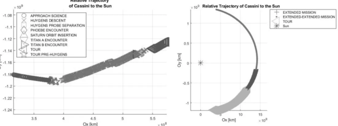
Figure 1. Movement of Cassini-Huygens spacecraft. a) The motion of the spacecraft, while the engine is turned off, was dominated by gravity along with the momentum; b) Histogram shows the relationship between intensity of Cassini movement among sampling, measuring the spacecraft movement give the opportunity for researchers to trace Saturn gravitational

field

With the gravity assistance of the planets of the Earth, Jupiter and Venus it required Cassini 6.7 years to reach Saturn, the following Figure 2 shows the mission phases magnitude correlated with samples, the IDs for the phases have been extracted from the metadata mission file, and it includes 14 phases.

Figure 3 depicts Cassini mission phases and the relative trajectory of Cassini to Sun, the mission is destined to explore the planet Saturn with its amazing rings and its various moons with distinctive and close attention on Titan.

Different shapes were allotted to show the correlation between the phases and their IDs. Subsequent to the launch which happened on 15 October 1997, a flyby period Cassini orbiter has spent near to three planets before arriving to Saturn system on 1 July 2004. When the nominal mission has accomplished by the date of July 2008, the orbiter had finished 75 orbits on its journey around Saturn. Primarily the mission was timetabled for a 4 years period that extends from 2004 till 2008, which is known as (primary mission), Since the mission was quite felicitous, so it was protracted twice, the first extension for the expedition took place in July 2008 and proceeded till October 2010, it is known as Equinox mission. The main purpose of this extension was to monitor the system of the planet Saturn during the time that the Sun passes the equatorial plane of Saturn. The next and final extension termed as Solstice mission and had lasted until 2017, with a crucial intent to observe the seasonal variations resulted from mutating solar illumination, up to the Sun amounts to its greatest vertical extent elevation on/at the top of Saturn's equatorial plane.

The generated graphic of the Figure 4(a) characterizes Cassini's flight mission path around the sun on its total mission length, which has started on 15 October 1997, and ended on September 15, 2017, while the insertion to Saturn orbit has happened on 1 Jul 2004.

Figure 2. Phases of the interplanetary mission Cassini-Huygens. 10% of the mission time: 14 phases, 90% of the total time: just 3 phases. phase 5 contains just two samplings

(31641…31644) making it invisible in the current scale of representation

Figure 3. Trajectory of the mission phases. a) First 35,000 of samples, it is found that the samples can be classified into groups based on the phase names of the mission. b) Samples

starting with 35,001 till 407,304

Figure 4. Trajectory parameters of the spacecraft Cassini-Huygens. a) The start of the path in the first graphic is pointed with the shape of a circle, while the end of the path is pointed with the shape of small square. b) The generated graphics represent the distance measured in KM between the sun and Cassini spacecraft during the whole mission when the

mission finished, Cassini spacecraft had crossed a distance of (7.8 billion kilometers) with regard to the Sun. The relationship among the independent variable sampling number and the dependent variable distance(D) is modeled as the 5th degree polynomial in sampling

number, fit function returns the coefficients for a polynomial p(sample#) with the degree 5 (to fit a polynomial to data of degree 5), which is considered the optimal fit (among the least square error R2 estimate). The polynomial coefficients have an inclined descendant of

powers p(D)=p₁D_n + p₂D_n-1 + .... + p_nD_n+1

During this journey, the spacecraft used the gravity-support flybys of various plants (Earth, Jupiter, Venus) with the purpose of boosting the velocity of the spacecraft proportionally to the sun in order to arrive at Saturn planet. Regarding the graphic in the Figure 5 concerning the position and velocity, it is known now from a scientific point of view that scientists might measure a car speed corresponding to the street that it uses. On the other hand, measuring the speed of a spacecraft is more complicated as it requires dual measurements proportional to the land and air in which it flies over and through respectively.

The velocity can be defined as a vector, thus the variation could be in the magnitude in addition to direction if that change is characterized by the feature of positivity, then the space shuttle is accelerated, while if it is characterized as negative then there is a reduction in the speed, it relies on the route that the spacecraft is taking, if the spacecraft in the forepart of the luminary, the spacecraft will waste speed, while if its position is behind the luminary, then it earns speed. It is known that any spacecraft that travels in the deep space, can be in contact with the planet of the Earth by dispatching radio signals, these signals could provide us with the spacecraft velocity by two methods.

The first method is straightforward, as the signals move the same speed of the light, then we could specify how much is the distance between this object and the Earth by the time period it takes for the radio signal to reach to it, rebound and march back, if the signal requires a greater period today than it took yesterday.

Then we can specify how much the spacecraft has moved in a single day also we can conclude the velocity, a further precise method of informing spacecraft velocity is via utilizing the Doppler effect, which is exploiting information concerning frequency shift of electromagnetic signals generated by moving spacecraft, based on that we could deduce the velocity.

In view of the fact that Cassini exploits the moon (Titan) gravity as hub spot for its considerable trajectory changes. Only one adjacent flyby of Titan will supply Cassini with a velocity change nearly could almost reach the propellant power that Cassini had at the phase of launching, so if Cassini pass by Titan with an inaccurate speed, then Cassini may end up moving in an incorrect way, consequently the navigation team back on Earth is in charge of taking such decisions regarding relative speeds to make sure that such errors doesn’t occur. Cassini would burn a little fuel to adjust the mistake. Normally, Cassini exploits propellant just to perform some slight rectifications to get back to the correct trajectory, the off-target is estimated by one kilometer. But if it fails to hit the target by tens of miles, current trajectory must have to be rescheduled or deleted; as resetting the trajectory may need another 6 months.

In Figure 6, we plotted the velocity of the Cassini spacecraft to Sun, as each object’s velocity should be designated with respect to other objects, the velocity is specified in kilometers per second, Cassini's velocity changed from 18.85 kilometers per second at the beginning of the maneuver to 18.4 kilometers per second at the terminus of the engine firing. The velocity was approaching 450 meters per second