DSc dissertation

(1)

DSc dissertation

Non-equilibrium dynamics of low dimensional quantum systems

Bal´ azs D´ ora

Budapest University of Technology and Economics Department of Physics

2014

(2)

(3)

Chapter 1 Introduction

1.1 Monolayer graphene

The first isolation of monolayer graphene (MLG), a single sheet of carbon atoms forming a honeycomb lattice, in 2004[1, 2] has attracted a huge interest, and practically revolutionized physics and has affected the research of many physicists. This is partly due to the fact that graphene is the first stable two dimensional crystal, awaiting our exploration, and partly because a general agreement has been reached in the closer condensed matter and broader physics community that the basic model describing its charge carriers is an effective, two dimensional, massless Dirac equation. Therefore, in contrast to e.g. highTc superconductors, where one has to struggle to justify the actual model choice, not mentioning the various approximation schemes, graphene’s low energy dynamics was soon demonstrated to be accountable for by the Dirac equation, as evidenced by numerous experimental, theoretical and ab initio studies.

Figure 1.1: Ripples in graphene

Even its existence is surprising, since the Mermin-Wagner theorem does not allow for positional long-range order in two dimensions, thermal fluctuations are expected to destroy long range crystalline ordering. A possible way

(6)

out is provided by realizing that graphene is still of finite size, therefore as long as the coherence length of ordering is longer than the actual system size, it looks a stable two dimensional crystal. Moreover, improved experimental techniques have revealed that graphene is not strictly two-dimensional but hosts ripples i.e. surface waves, and stabilizes itself by fluctuations in the third spatial dimension, as shown in Fig. 1.1, which are typically 20-200 ˚A long and 10 ˚A high bumps

x y

a1

a2

A

B

a a t t

t

K’ K

−5

0 5 −5 0 5

−3

−2

−1 0 1 2 3

kx k_y

E(k)

Figure 1.2: Top: a small segment of the honeycomb lattice in shown, made of two interpenetrating triangular lattices, with the two triangular sublattices denoted by filled and empty circles, together with the translational lattice vectors a1 and a2. The green lines separate the unit cells. Bottom left:

the low energy part of the spectrum in momentum space with the two non- equivalent Dirac cones at the opposite corners of the Brillouin zone. Bottom right: The full energy spectrum in the Brillouin zone.

(7)

Soon after its discovery, a variety of interesting effect were predicted and subsequently observed experimentally, such as unconventional quantum Hall effect[2], a (possibly universal) minimal conductivity at vanishing carrier concentration[3], Klein tunneling in p-n junctions[4, 5] and Zitterbewegung[6, 7], frequency independent optical conductivity over a wide frequency range etc.

All these are natural consequences of the low energy physics of the half- filled honeycomb lattice, studied in the tight-binding approximation. The honeycomb lattice, depicted in Fig. 1.2 is regarded as two interpenetrating triangular lattices, whose lattice sites form the two sublattices. By considering only nearest neighbour, intersublattice hoppings, the resulting Hamilto- nian is written in momentum space in second quantized form as

Hgraphene=X

k,σ (a⁺_k,σ, b⁺_k,σ)

0 tf(k) tf^∗(k) 0

ak,σ

bk,σ

, (1.1)

where the ak,σ and bk,σ operators annihilate particles from sublattice A and B with momentum kand spin σ, f(k) = 1 + 2 exp(i3k_y/2) cos(√

3k_x/2), and we use the convention to take the nearest neighbour carbon atom distance to unity (which is 1.42 ˚A), and t ≈ 2.7 eV the hopping integral between neighbouring carbon atoms. Therefore, the spectrum consists of two bands as E±(k) = ±t|f(k)|. The two bands touch each other at the corners of the hexagonal Brillouin zone, among which three-three are connected by reciprocal lattice vectors, ending up with two non-equivalent touching points at K and K^′. By expanding the spectrum around these point, using e.g.

f(K+p)≈(3/2)(px+ipy), we arrive to a linearly dispersing band-touching as E_±^K(p) = ±3t|p|/2 at around point K, and similarly for point K^′. The low energy physics is determined by excitations living close to these Dirac points, described by an effective Dirac equation, given by

H_graphene= X

p,σ,τz

Ψ⁺_p,σ,τ_z

0 vF(px−τzipy) vF(px+τzipy) 0

Ψ_p,σ,τ_z, (1.2) where vF = 3t/2 ∼ 10⁶ m/s is the Fermi velocity, τz = 1, -1 denotes the K and K^′ points and represents the valley degree of freedom and the spinor Ψp,σ,τz = (ap,σ,τz, bp,σ,τz) contains operators with momentum close to the Dirac point at K (τz = 1) or K^′ (τz =−1). By focusing on the e.g. τz = 1 term, namely a single a single Dirac cone, which is written in first quantized form as

HDirac =vF

0 pˆx−iˆpy

ˆ

px+ipˆy 0

=vFσ·p,ˆ (1.3)

(8)

where σ = (σ_x, σ_y) are Pauli matrices, most of graphene’s properties can be analyzed by borrowing from high energy physics or QED to some ex- tent, where the appearance of the Dirac equation is part of the daily rou- tine. However, there are several significant differences between graphene’s Dirac equation and its relativistic version: first, graphene’s charge carriers are massless in the relativistic sense, namely that E(p)∼ |p| down to small momenta, whose fully relativistic realization among elementary particles is hotly debated. Note that in the condensed matter sense, these are infinitely heavy particles since the inverse of the effective mass tensor, calculated as

m⁻¹ = vF

|p|³

p²_y −pxpy

−pxpy p²_x

, (1.4)

has zero determinant and is therefore non-invertible. Second, the maximal velocity for graphene’s particles is the Fermi velocity, being 1/300th the velocity of light, therefore bringing the typical energy scales, required to in- vestigate graphene, down to the conventional energy scales of a condensed matter experiment, thus allowing for the observation of relativistic phenomena in low temperature labs. Third, the matrix structure in Eq. (1.2) stems from a peudospin variable, accounting for the two non-equivalent sublattices of the honeycomb lattice and not from the the physical spin of the particles. Due to this sublattice structure, these are called chiral Dirac electrons, since the helicity operator, σ·p/|p| commutes with the Hamiltonian and is a good quantum number. For graphene, this implies σ kpfor a given eigen- state. Note that by taking additional complications in the band structure into account (e.g. hoppings etc), the Dirac points are shifted in energy, but otherwise remain intact.

Due to the linear energy-momentum relationship and the two-dimensionality of graphene, its density of states (DOS) per unit volume vanishes linearly close to half filling as

ρ(ω) = 1 2π

|ω|

v_F² (1.5)

per spin and valley, similarly to d-wave superconductors or d-density waves[8].

In this respect, graphene is neither a metal with a sizeable DOS at the Fermi energy, nor an insulator with strongly suppressed DOS, but can be regarded as a semimetal.

The linear band crossing, provided by the Dirac equation in Eq. (1.3), possesses a half-integer quantized Berry flux[9]. The wavefunction is written in momentum space as

|α,pi= 1

√2

α exp(iϕp)

, (1.6)

(9)

x

| Ψ (x)|

2

Schrodinger ..

Dirac

Figure 1.3: Schematics of Klein tunneling in graphene. At normal incidence, the transmission probability is always one for chiral particles, regardless to the width or height of the barrier.

whereα =± corresponds to positive and negative energy states asEα(p) = αvF|p| and ϕp = arctan(py/px). The Berry phase is calculated from

−i I

C

dp· hp, α|∇_p|α,pi=±π, (1.7) whereC is a contour in momentum space enclosing the Dirac point and the

± sign depends on the orientation of the contour. The π Berry phase is regarded as a hallmark of two-dimensional massless Dirac fermions.

Another particularly interesting feature of Dirac fermions, stemming from their chiral nature, is their insensitivity to external electrostatic potentials due to the so-called Klein tunneling[5], meaning that Dirac fermions can be transmitted with probability 1 through a classically forbidden region, as illustrated schematically in Fig. 1.3. This happens because positive energy states can tunnel into negative energy states without changing their quantum numbers. In particular, for a potential barrier of widthDand height V0, the transmission probability of an incoming electron with energy |E| << |V₀| is[3, 10]

T(φ) = cos²(φ)

1−cos²(Dqx) sin²(φ), (1.8) whereφis the angle of incidence andqx ≈q

(V0/vF)²−k²_y is the longitudinal

(10)

Figure 1.4: Left: the minimal conductivity of various quality graphene sam- ples at the Dirac (charge neutrality) point. Right: the longitudinal resistivity and Hall conductivity of graphene in quantizing magnetic field as a function the carrier density.

component of the momentum within the barrier and ky is the conserved component of the momentum, parallel to the barrier. Note that forDqx =nπ with n an integer, the barrier becomes completely transparent since T(φ) = 1, independent of the value of φ. In addition, for normal incidence with φ → 0 and for any value of Dqx, barrier is again totally transparent. This result is a manifestation of the Klein tunneling[5], which does not occur for nonrelativistic electrons, where for normal incidence, the transmission is always smaller than 1. Due to Klein tunneling, Dirac electrons cannot be confined by conventional potential barriers[11], provided by gating the sample, as opposed to conventional semiconductor technology.

Since helicity is a good quantum number in the low energy Dirac equation description of graphene, backscattering is forbidden since it would require changing the sign of the helicity of a given momentum state, which cannot be provided by simple potential scatterers. Due to this, Dirac electron transport in graphene can be ballistic for typical sample sizes. Since disorder is unavoidably present in any material, there has been a great deal of interest in trying to understand how disorder affects the physics of Dirac electrons in graphene and its transport properties. Under certain conditions, Dirac fermions are immune to localization effects observed in ordinary electron

(11)

systems and it has been established experimentally that electrons can propagate without scattering over large spatial regions of the micron size. This originates from the intricate interplay of scattering and density of states: as the charge neutrality point is approached, a decreasing number of particles are available for charge transport due to the vanishing DOS, which, on the other hand acquire an increasingly long lifetime even in the presence of disorder. These two effects cancel each other perfectly, resulting in a finite, almost universal minimal conductivity at the Dirac point, largely independent from the microscopic details of the sample, as illustrated in Fig 1.4.

Since graphene is inherently two-dimensional, it represents an ideal plat- form to study quantum-Hall physics. A semiclassical Bohr-Sommerfeld quantization of the cyclotron orbits predicts that the Landau levels follow an unusual sequence as En ∼ √

n+ Γ, where n is the Landau level index and Γ is related to the Berry phase and can only be determined from quantum mechanical considerations. These yield

En= sign(n)vF

p2|n|eB⊥, (1.9)

whereB⊥is the perpendicular component of the magnetic field to the graphene plane, andn is an integer. As opposed to a normal two-dimensional electron gas (2DEG), these levels are not equidistant, and depend on√

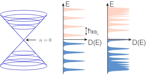
B⊥in contrast to the linear dependence of the 2DEG and do not possess zero point energy, as follows from a Dirac oscillator vs. Schr¨odinger oscillator scenario. Each Landau level is fourfold degenerate, coming from the combined effect of the valley (2) and spin (2) degrees of freedom. The zero mode, provided by the n = 0 Landau level is special since it is half electron- and half hole-like, as it sits right at the intersection of the upper and lower Dirac cones, i.e. at the Dirac point (see Fig. 1.5) When calculating the Hall conductivity, each Landau levels contributes with a step of 4×e²/2h to the Hall conductivity, where the factor of 4 comes from the valley and spin degeneracies, and the 2 in the denominator results from the π quantized Berry phase. The Hall conductivity is qualitatively well described by

σ_xy = 2e²

h sign(B)

N

X

n=−N

sign (E_n−µ) (1.10) producing the unconventional Hall steps in graphene as a function of the chemical potential µ, as shown in Fig. 1.4, and N is a symmetric cutoff.

The first quantum Hall step, starting from the Dirac point withµ= 0, is only 2e²/h large as opposed to the subsequent steps in the series with 4e²/h size. This roots back to the peculiar zeroth Landau level with n = 0, which

(12)

is only half particle like, therefore contributes only with a half step to the plateaux sequence. Note that if there was no spin and valley degeneracy, the contribution of this zeroth Landau level would be a half-integer quantized Hall conductivity as e²/2h. Apparently, Dirac points always appear in pairs due to a no-go theorem[12], therefore the smallest step is expected to bee²/h in general.

The lowest (small n) Landau levels in graphene are separated by an energy gap of order 300-400 K in a magnetic field of 1 T, in contrast to a two-dimensional electron gas, where the equidistant Landau levels are separated by a gap of the order of the magnetic field itself. Due to the peculiar quantization of Dirac fermions, the quantum-Hall effect remains observable even at room temperatures[13]. These are illustrated with the density of states of Landau quantized Dirac and normal two-dimensional electrons in Fig. 1.5.

n = 0

h w

c

E

D(E) D(E)

E

Figure 1.5: Left: the Landau level structure in the Dirac cone. Right:

the DOS in a Landau quantized normal two-dimensional electron gas and graphene.

Graphene’s two dimensionality notwithstanding, it was possible to mea- sure its optical conductivity, which exhibits a frequency independent optical response over a wide frequency range. This can be understood from simple considerations: the electric current operator in the x direction for Dirac fermions is jx = evFσx, independent from the momentum. Its matrix ele- ment, corresponding to interband transition is |hp,+|jx|p,−i|² = sin²(ϕp).

The total number of states, participating in this process is proportional to the size of the Fermi surface ∼ |p|. Putting this together and using the linear relationship between energy and momentum, the total number of states,

(13)

probed by an electromagnetic wave with frequencyω, scales with |ω|. Divid- ing it by the frequency gives the optical conductivity, which indeed becomes frequency independent. By working out the prefactor, the optical conductivity is

σxx(ω) = πe²

2h. (1.11)

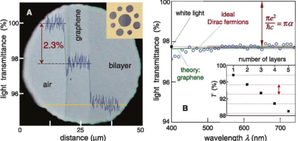
Not surprisingly, since the Dirac equation does not contain any intrinsic energy scale which would influence the optical response, the optical conductivity is also universal. The optical transparency is calculated from this as T^opt = 1−πα, where α =e²/~c≈ 1/137 is the fine-structure constant. De- spite being only one atom thick, graphene is found to absorb a significant 2.3% fraction of incident white light, By stacking graphene to obtain multi- layer graphene, the optical transparency reduces linearly with the number of layers for up to 5 layers, as shown in Fig. 1.6.

Figure 1.6: Left: Photograph of an aperture partially covered by mono and bilayer graphene. The line scan profile shows the intensity of transmitted white light. Right: Optical transmittance as a function of the number of graphene layers. From Ref. [14]

Most of graphene’s electronic properties can be analyzed using a single particle picture based in the Dirac equation, and surprisingly good agreement is reached when comparing to experimental results. This is even more surprising in light of the fact that since its effective ”light” velocity (i.e. the Fermi velocity) is 300 times smaller than the speed of light, its fine structure constant should be 300 times bigger than that in QED, of the order of 1-2, suggesting that interaction effects would play an important role and should

(14)

be non-perturbative. While in most condensed matter systems, interaction effect are omnipresent and obvious, one has to struggle with graphene to see any sign of interactions. From the point of view of basic research, the re- sent discovery of fractional quantum Hall physics in graphene sounds really promising[15, 16], allowing for studying strongly interacting Dirac fermions in quantizing magnetic field with no obvious analogue on high energy physics.

In addition to its unique electronic properties, which is the main concern of this dissertation, graphene also exhibits unique mechanical properties and is said to be the strongest material ever measured with a Young’s modulus in the TPa regime. Its two-dimensionality makes it an ideal candidate to engineer planar electronic devices. Since its bulk is its surface, it was shown to be capable of detecting individual gas molecules, attached to its surface.

Among many others, graphene could accelerate genomics by reading the whole human genome in two and a half hours. Whether graphene fulfills the promise it holds in applied sciences remains to be seen in the future, but it has certainly revolutionized condensed matter and related fields enormously over the past 7-8 years.

1.2 Bilayer graphene

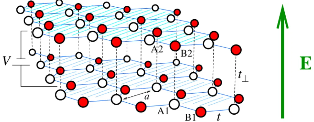
Bilayer graphene (BLG) is composed of two monolayer graphenes (MLGs) in Bernal or AB stacking, meaning that the A sublattice of one layer is on top of the B sublattice of the other layer, as shown in Fig. 1.7. This is the typical stacking pattern of 3D graphite as well. Its charge carriers, as we show below, reveal non-relativistic, ”Schr¨odinger” (quadratic dispersion) and relativistic ”Dirac” (chiral symmetry, unusual Berry phase) features.

Due to their peculiar nature, as discussed below, BLG holds the promise of revolutionizing electronics, since its band gap is directly controllable by a perpendicular electric field over a wide range of parameters [17, 18, 19, 20, 21]

(up to 250 meV [22]), unlike existing semiconductor technology. Moreover, unlike monolayer graphene, whose effective model, namely the Dirac equation was thoroughly investigated in QED and relativistic quantum mechanics, understanding the low energy properties of BLG represents a new challenge.

The band structure of BLG also follows from tight-binding calculations.

In addition to the intralayer hopping of the graphene layers, an interlayer hopping, t⊥ ≈ 0.3-0.4 eV should be taken into account, since the typical distance between the layers is d = 3.3 ˚A. Additional hopping processes are also present, but these are neglected for the sake of simplicity. A tight

(15)

A2 B2

A1 B1

V

t t

_⊥

a

E

Figure 1.7: The lattice structure of BLG with the relevant hopping processes, the vertical green arrow denotes a perpendicular electric field.

binding calculation for the kinetic energy gives

Hgraphene =X

k,σ

Ψ⁺(k, σ)







∆ tf(k) 0 0

tf^∗(k) ∆ t⊥ 0

0 t⊥ −∆ tf(k)

0 0 tf^∗(k) −∆







Ψ(k, σ), (1.12) where the Ψ⁺(k, σ) = (a⁺_1,k,σ, b⁺_1,k,σ, a⁺_2,k,σ, b⁺_2,k,σ), and the operators create particles on layer 1 or 2, sublatticeA orB with momentum kand spinσ, as visualized in Fig. 1.7, and f(k) has already been defined for MLG. Here, ∆ represents a layer dependent chemical potential, which arises upon switching on a perpendicular electric field. Due to the 4 atoms in the unit cell, BLG possesses 4 band, two of them touching each other at zero energy for ∆ = 0, and two others separated by±t⊥, as shown in Fig. 1.8

The low energy part of the spectrum in BLG is obtained by integrating out the high energy modes, leading to an effective 2×2 description as[18, 23]

H =

∆ (px−ipy)²/2m (px+ipy)²/2m −∆

, (1.13)

where m = t⊥/2v_F² ≈ 0.03me, and its spectrum is ±p

∆²+ (|p|²/2m)². In the presence of a finite electric field, the band touching disappears and a finite bandgap appears, whose size is easily tunable by the electric field. However, screening due to electron interactions becomes relevant in this case, and the induced gap is related to the external potential, Uext, created by the electric

(16)

-4 -2

0 2

4 -4 -2 0 2 4

-2 0 2

-4 -2

0 2

4 -4 -2 0 2

E_k

k_x

k_y

E_k

+t_⊥

−t_⊥

|k|

Figure 1.8: The energy spectrum of BLG in the Brillouin zone together with the low energy part of the spectrum around zero energy for ∆ = 0.

field as [18, 24]

2∆ =Uext+ e²dδn

2A_cε_rε₀, (1.14)

where δn = P

p(n1p −n2p) is the dimensionless density imbalance between the two layers with n_ip the particle density of state p on the ith layer. The induced gap to a good approximation is given by [18, 17]

∆ =

1 +λln 4t⊥

|Uext| −1

Uext

2 , (1.15)

and the density imbalance reads

δn= 4ρ0∆ ln (|∆|/2t⊥), (1.16) with λ = e²dρ0/Acεrε0 ∼ 0.1−0.5 the dimensionless screening strength, ε0

the permittivity of free space and ρ0 = Acm/2π~² the density of states per valley and spin in the limit ∆→0. For SiO2/air interface,εr≈2.5 (εr = 25 for NH3,εr = 80 for H2O), which reduces the effects of screening. This extra tunability of its bandgap makes bilayer graphene a promising candidate as well for future electronic devices. By applying a dual-gate structure [19, 22, 20, 25, 21] with top and back-gate, the size of the gap together with the total number of charge carriers can be tuned independently.

(17)

The physical properties of BLG with ∆ = 0 are as surprising as those of MLG, and vaguely speaking, in spite of the different topology of the low energy Hamiltonians in Eqs. (1.3) and (1.13), it is a ”factor of 2 times monolayer graphene”. It exhibits a universal minimal conductivity at the charge neutrality point, which is twice as large as that of MLG. Its wavefunction in momentum space is

|α,pi= 1

√2

α exp(i2ϕp)

, (1.17)

whereα =± corresponds to positive and negative energy states asE_α(p) = α|p|²/2m and ϕp = arctan(py/px). The Berry phase is calculated to be

±2π [26] and in spite of its massive quasiparticles, it exhibits chiral symmetry unlike particles obeying the standard Schr¨odinger equation. The Klein tunneling is also peculiar in BLG: no perfect transmission occurs for perpendicular incidence, in contrast to MLG, but perfect reflection. This perfect reflection (instead of the perfect transmission) is viewed as another manifestation of Klein tunneling, because the effect is again due to the chirality of the quasiparticles (fermions in MLG and BLG exhibit chiralities that resem- ble those associated with spin 1/2 and 1, respectively, as follows from the π and 2π Berry phases). For MLG, an electron wavefunction at the barrier interface matches perfectly the corresponding wavefunction for a hole with the same direction of pseudospin due to chiral symmetry, yieldingT = 1. In contrast, for BLG, the chiral symmetry requires a propagating electron with wavevector k to transform into a hole with wavevector ik(rather than−k), which is an evanescent wave inside a barrier.

Additionally, BLG is also characterized by a featureless optical conductivity which is twice that of MLG, as shown in Fig. 1.6. One essential difference, however, with respect to MLG is the finite density of states around half filling. Due to this, a short range electron-electron interaction is usually found to be marginally relevant, leading to all sorts of phase transition in BLG, at least on a theoretical level [27, 28, 29, 30]. The experimental verification of such phase transitions still remains to be seen.

The Landau level structure in a perpendicular magnetic field also shows Dirac like (chiral) and Schr¨odinger like features. In the absence of a gap, the Landau levels per spin and valley read as

Enα =αp

n(n+ 1)eB⊥/m (1.18)

with α = ± and n non-negative integer and B⊥ is the perpendicular component of the magnetic field to the BLG sheet. First of all, it contains two degenerate zero modes (in contrast to the single zero mode in graphene),

(18)

−4 0

−3

−2

−1 0 1 2 3 4

n (arb. units) σxy(4e2 /h)

Figure 1.9: The Hall conductivity is shown schematically for MLG (blue) and BLG (red) as a function of the particle density, n, measured from half filling

while the low energy part of the spectrum increases is highly non-equidistant in the Landau level index. This, however, crosses over to a∼nincrease with the Landau level index for largen, thus producing Schr¨odinger-like behaviour at high energies. The resulting quantum Hall effect is also different from that in graphene. Due to the doubled amount of zero modes, the first quantum Hall step is 4e²/h large (twice as big as that in MLG) from the charge neutrality point, while all other steps have the same size as for graphene, since the degeneracies of the finite energy states are identical for MLG and BLG.

The Hall conductivities are depicted in Fig. 1.9.

1.3 Topological insulators

Before the discovery of the integer quantum Hall effect, various phases of materials were classified according to their broken symmetries. For example, a crystal breaks the rotational and translational symmetry of free space, superconductors break the gauge invariance, a magnet breaks the spin rotational and sometimes the translational invariance etc. In 1980, the observation of the perfect quantization (up to 9 digits) of the integer quantum Hall effect[31]

made us reconsider this issue, and the question ”What causes quantization”

called for an answer. Based on the seminal work in Ref. [32], it was realized that quantization results from topological order, and some response functions are determined by a topological invariant, explaining quantization.

The response function is independent of the sample-dependent microscopic

(19)

parameters, such as scattering rate, interactions strength etc. due to topological protection. Such materials are termed topological insulators. Another, closely related definition states that a topological phase is an insulator in its bulk, which develops metallic surface or edge states when it gets in contact with a normal (i.e. topologically trivial) phase or vacuum. The connection between the two definitions is provided by the bulk-edge correspondence, which states that the integer value of the topological invariant is given by the number of surface or edge states. For example, a 2e²/h Hall conductivity implies two conducting, ballistic, chiral channels around the edges of the sample, immune to backscattering.

The early members of the topological insulator (TI) family were the celebrated quantum Hall states, but due to recent experimental and theoretical progress [33, 34], numerous relatives have recently emerged. The topological protection of these materials mostly arises from their specific band structure, deriving from a strong spin-orbit interaction. Application-wise, TIs hold the promise to revolutionize spintronics, and contribute to conventional and quantum computing.

We start by introducing two-dimensional TIs with one-dimensional edge states. The first member of the TI insulator family is graphene. When supplemented with the intrinsic spin-orbit coupling (SOC), its Hamiltonian reads as[35]

H =vF(σxpx+σyτzpy) + ∆σzτzSz, (1.19) where τz = ±1 distinguishes between the K and K^′ valleys, Sz is the physical spin and ∆ is the intrinsic SOC. This preserves parity and time reversal symmetry, and leads to a fully gapped spectrum in each valley as

±p

v_F²|p|²+ ∆², suggesting that it turns graphene into an insulator. How- ever, when we leave the continuum limit and consider the original tight- binding problem on the hexagonal lattice, the above SOC can be originated by second nearest neighbour, intrasublattice hopping processes, which change sign according to whether the hopping occurs clockwise or anticlockwise on the hexagonal lattice. The SOC in Eq. (1.19) is related to a model introduced by Haldane [36] as a realization of the parity anomaly in (2+1) dimensional relativistic field theory. Since Eq. (1.19) conserves Sz, each spin species can be treated separately. The Hamiltonians for Sz = ±1 violate time reversal symmetry and are equivalent to Haldanes model for spinless electrons, which could be realized by introducing a periodic magnetic field with no net flux.

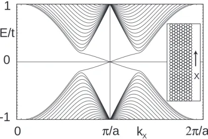
The energy spectrum of the lattice model, reducing to Eq. (1.19) in the continuum limit, is evaluated by considering a finite width graphene nanorib- bon, revealing the presence of edge states. Fig. 1.10 shows the one dimensional energy bands for a strip where the edges are along the zig-zag direction

(20)

in the graphene plane. The bulk bandgaps at the one dimensional projec- tions of the K andK^′ points are clearly seen. In addition to this, two bands traverse the gap, connecting theK andK^′ points. These bands are localized at the edges of the strip, and each band has degenerate copies for each edge.

The edge states are not chiral since each edge has states which propagate in both directions. However, the edge states are ”spin filtered” in the sense that electrons with opposite spin propagate in opposite directions.

-1 0

0 π /a 2π /a

E/t

k 1

X

Figure 1.10: One dimensional energy bands for a strip of graphene (shown in inset). The bands crossing the gap are spin filtered edge states, from Ref. [35].

The effective model for the edge states is

Hef f =vFSzpx, (1.20)

protected by time reversal invariance, i.e. a right/left-going electron car- ries spin up/down, and backscattering can only occur if the spin is also flipped, therefore simple potential scattering cannot spoil the ballistic motion along the edges. The spin-Hall conductivity, calculated from either the bulk model[9] using Eq. (1.19) or using only the existence of ballistic edge states from Eq. (1.20), reads as

σ^spin_xy = e

2π, (1.21)

being quantized. Note that this quantization is less robust than that of the quantum-Hall effect, since magnetic scatterers can provide us with effi- cient backscattering by flipping the electron spin, and degrade the quantized

(21)

spin-Hall response. So far, graphene as a spin-Hall insulator exists only in our dreams, since the size of the intrinsic SOC is estimated to be in the µeV range[37], being overwhelmed by additional processes such as impurity scattering etc. Nevertheless, cold atomic systems can be used to engineer graphene like system with intrinsic SOC [38].

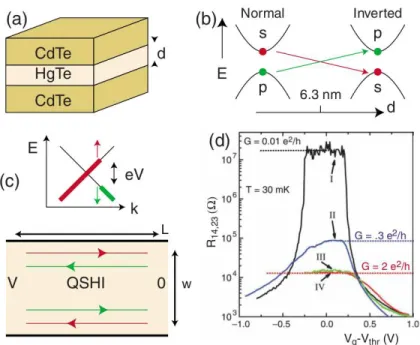
Another member of the spin-Hall insulator family features a real material, where the existence of edge states was predicted theoretically[39] and subsequently demonstrated experimentally[40], namely HgTe/CdTe quantum wells. The Hg1−xCdxTe belongs to the family of semiconductors with strong spin-orbit interactions. Its band structure is rather common among semiconductors: the conduction/valence band states have an s/p-like symmetry. In HgTe, however, the p levels are above the s levels, resulting in an inverted band structure. Ref. [39] considered a quantum well structure where HgTe is sandwiched between layers of CdTe. When the thickness of the HgTe layer isd < dc = 6.3 nm, the 2D electronic states bound to the quantum well have the normal band order. On the other hand, ford > dc, the 2D bands invert.

The inversion of the bands with increasingdsignals a quantum phase transition between the trivial insulator and the quantum spin Hall insulator. This follows from the observation that the system has inversion symmetry: since the sand p states have opposite parity, the bands will cross each other atdc

without an avoided crossing, causing the energy gap to vanish at d=dc. The experimental results from Ref. [40] are depicted in Fig. 1.11, demon- strating convincingly the existence of the edge states of the quantum spin Hall insulator.

Three dimensional topological insulators posses two dimensional surface states, described by a two-dimensional Dirac equation as[33, 34]

H=v_F(S_xp_y−S_yp_x) + ∆S_z, (1.22) where S stands for the physical spin, and ∆ is a mass gap, originating from a thin ferromagnetic film covering the surface of TI, lifting the Kramer’s degeneracy of the Dirac point. After a π/2 rotation of the spin around S_z, it reduces to the conventional form of the Dirac equation in Eq. (1.3). The spin dependence comes, similarly to the two-dimensional case, from strong spin- orbit coupling, therefore, materials with large atomic number are beneficial, such as Bi[33, 34].

Among their fascinating properties, such as the surface quantum Hall effect, coming from Eq. (1.22) in a perpendicular magnetic field, three- dimensional topological insulators feature the topological magnetoelectric effect. This means that the electron spin can be manipulated by an electric field and conversely, the electric current can be controlled by a magnetic

(22)

Figure 1.11: Experiments on HgTe/CdTe quantum wells. a) Quantum well structure. b) As a function of layer thickness d the 2D quantum well states cross at a band inversion transition. The inverted state is a quantum spin- Hall insulator with helical edge states, whose non-equilibrium population is determined by the leads (c). d) Experimental two terminal conductance as a function of a gate voltage that tunes the Fermi energy through the bulk gap.

Sample III and IV show quantized transport associated with edge states.

From Ref. [40].

field. This comes from the observation that the electric current operator for the surface states is jx,y ∼ ∂H/∂px,y ∼ Sy,x, therefore a vector potential, describing a time dependent electric field, which couples normally to the electric current, couples directly to the electron’s spin. Conversely, the Zeeman coupling to a magnetic field, B, involves S·B terms, affecting the charge dynamics.

1.4 Landau-Zener dynamics and Kibble-Zurek scaling

As we have seen previously, the basic equation governing the charge carriers in graphene and its variants as well as topological insulators is a 2×2

(23)

Dirac equation. Whenever some spatial or temporal dependent potentials are added to it, one needs to solve two coupled differential equations, as is the case for e.g. a time dependent vector potential, describing an electric field and spatially dependent scalar potential, accounting for a p-n junc- tion in graphene[41]. The simplest and probably the most widely used time dependent 2×2 Hamiltonian is the Landau-Zener model[42, 43], which is to time-dependent quantum phenomena what the harmonic oscillator is to quantum mechanics. Note that the case of a scalar potential can also be mapped to this in the momentum representation[44]. It describes a two-level system, going through an avoided level crossing. Its Hamiltonian is

HLZ =

−vt ∆

∆ vt

, (1.23)

andv >0. Its instantaneous eigenenergies are given byǫ±(t) =±p

∆² + (vt)². Its eigenvectors are |1i= (1,0)^T with positive eigenenergy and |0i = (0,1)^T with negative eigenenergy, and the time evolution starts att→ −∞with|0i being occupied. Was the time evolution completely adiabatic, i. e. v → 0, then at time t → ∞ the system would be in its ground state as |1i with probability one. In case of diabatic time evolution with v → ∞, the final state att→ ∞would still coincide with the initial state as|0i. For any finite rate passage, there will be a finite probability to stay in the initial state and to tunnel to the other state. The celebrated Landau-Zener formula describes the probability to tunnel into the excited state and is given by

Pad = exp

−π∆² v

. (1.24)

This can be obtained from the exact solution of the model, which is, however, not very illuminating since it involves the parabolic cylinder functions[45, 46].

By using some approximate, semiclassical methods such as the WKB[47]

or its temporal version known as the Landau-Dykhne method[48, 49], the required probability is determined from

Pad = exp



−2Im

t+

Z

t₋

ǫ+(t)dt



, (1.25)

which describes the tunneling between the adiabatic energy levels, fromǫ−(t) toǫ+(t), which is determined by the classically forbidden regions. The limits of integration is determined after continuing the adiabatic eigenenergies to complex time and look for a crossing point between the two bands asǫ+(t) =

(24)

0. This occurs when t± = ±i∆/v. The above expression is correct within exponential accuracy in general since it neglects the interference between multiple quantum tunneling processes. Interestingly, this gives the exact result for the Landau-Zener model, e.g. for the present case. The above integral is evaluated easily since it only requires the knowledge of the area of a semi-circle, giving Eq. (1.24).

The Landau-Zener model is closely connected to the celebrated Kibble- Zurek scaling[50], and is often considered to be the microscopic basis to to derive it for specific models after mapping them to the Landau-Zener model[51], which is the case for a magnetic field quench in the transverse field Ising chain[52, 53] as an example. A quench here means a time-dependent change of some parameters in the Hamiltonian. If it is abrupt, we face a sudden quench. The Kibble-Zurek argument[54, 55] predicts a scaling form for the defect density following a slow quench through a quantum critical point. A finite rate passage through a quantum critical point (QCP) results in closing the gap, with an activated behaviour and a finite correlation length giving way to metallic response and power-law correlations exactly at the QCP. Due to the non-equilibrium nature of the process, defects (excited states, vortices) are produced. When the relaxation time of the system, which encodes how much time it needs to adjust to new thermodynamic conditions, becomes comparable to the remaining ramping time to the critical point, the system crosses over from the adiabatic to the diabatic (impulse) regime. In the latter regime, its state is effectively frozen, so that it cannot follow the time-dependence of the instantaneous ground states – as a result, excitations are produced[50]. Evolution restarts only after leaving the diabatic regime, with an initial state mimicking the frozen one. The theory, general as it is, finds application in very different contexts in physics, ranging from the early universe cosmological evolution[54] through liquid^3,4He [56, 55, 57] and liquid crystals[58, 59] to ultracold gases[60], verified for both thermodynamic and quantum phase transitions[61].

Having argued that defects should be generated, we now sketch the deriva- tion of the Kibble-Zurek scaling. Let ∆ be the characteristic energy scale associated with the proximity to the critical point, which can be a gap or some other crossover scale. The evolution becomes non-adiabatic close to the critical point when the ’reaction time’ of the quantum system given by the inverse of the energy gap is comparable with the timescale at which the Hamiltonian is changing: 1/∆∼ ∆/(d∆/dt)[62]. Assuming linear quenches of the form ∆ ∼ |t/τ|^zν, where τ measures the adiabaticity of the quench, the typical crossover time istc ∼τ^zν/(zν+1), wherez andν are the dynamical and correlation length exponents, respectively. The healing length, ξ typically denotes the length over which a single defect is present, which gives

(25)

g

τ relax τ_quench

adiabatic adiabatic

diabatic

Figure 1.12: A cartoon for the Kibble-Zurek dynamics,g is a control parameter and the QCP is located atgc, thus ∆∼g−gc. When the relaxation time, τrelax ∼1/∆ becomes comparable to the quench time, τquench ∼ ∆/(d∆/dt) (which is constant for a linear quench), the evolution becomes diabatic and defects are produced.

ξ ∼ τ^ν/(zν+1). The density of defects in a d-dimensional system scales as 1/ξ^d which leads to the Kibble-Zurek scaling form for the density of defects n given by

n∼ξ^−d∼τ^dν/(zν+1). (1.26)

The process is shown schematically in Fig. 1.12.

1.5 Luttinger liquids: basic properties

Understanding non-equilibrium dynamics and quantum many body effects represent equally exciting problems of contemporary physics. When these two fields are combined, namely when strongly correlated systems are driven out-of-equilibrium, we face a real challenge. Experimental advances on ultracold atoms [63] have made the time dependent evolution and detection of quantum many-body systems possible, and in particular, quantum quench- ing the interactions by means of a Feshbach resonance or time dependent lattice parameters has triggered enormous theoretical [64, 65, 51, 66] and experimental [67, 68, 69, 70] activity.

Luttinger liquids (LLs) are ubiquitous as effective low-energy descriptions of gapless phases in various one-dimensional (1D) interacting systems [71, 72].

In 1D fermions, e.g., Landau’s Fermi liquid (FL) description breaks down for any finite interaction, and the low-energy physics is described by bosonic collective modes with linear dispersion, and is characterized by anomalous

(26)

non-integer power-law dependences of correlation functions. This is to be contrasted to a Fermi liquid, where the quasi particle picture (electron) holds, implying critical exponents fixed to an integer. The LL similarly arises as the low-energy description of interacting 1D bosons or that of spin chains [71].

The breakdown of the FL description is best exemplified by the equal- time single particle correlation function, which, at T = 0, behaves in real space as

hΨ(x, t)Ψ⁺(0, t)i^{F L}∼ Z

x, (1.27)

for a FL, where Z ≤ 1 is Landau’s quasiparticle weight[73], and Ψ(x, t) is the fermionic field operator, which annihilates a particles at x in real space and at t in real time. In a LL, it decays as

hΨ(x, t)Ψ⁺(0, t)iLL ∼ 1

x^1+γ², (1.28)

where γ depends on the interaction strength. Its spatial Fourier transform corresponds to the momentum distribution function, which exhibits a finite jump at the Fermi wavevector kF in a FL, signalling the existence of long- living fermionic excitations. In contrast, fermionic quasiparticles are not welcome in a LL, thus Z vanishes, as shown in Fig. 1.13.

k F k F

n(k)

k k

Luttinger liquid Fermi liquid

Z

T=0

n(k) }

Figure 1.13: The momentum distribution function is depicted schematically for a FL (left) and LL (right). The finite jump at kF, characteristic of the FL disappears in a LL, giving way to a smooth power law behavior.

A similar distinction can be made in the time or frequency domain as well. The decay of the real time correlator,

hΨ(x, t)Ψ⁺(x,0)i^{F L}∼t⁻¹ (1.29)

(27)

in a FL is to be contrasted to the LL behaviour as

hΨ(x, t)Ψ⁺(x,0)i^LL ∼t^−(1+γ²⁾, (1.30) changing the integer exponent to an arbitrary real number. Its temporal Fourier transform defines the density of states (DOS), whose behaviour is shown in Fig. 1.14. While the DOS is typically finite in a FL at the Fermi energy, it vanishes in a power law manner in a LL, developing pseudogap behaviour, because fermions are not good quasiparticles.

Luttinger liquid

Fermi liquid T=0

F

ω

ω ω ω

ρ(ω) ρ(ω)

Figure 1.14: The quasiparticle density of states is shown schematically for a FL (left) and LL (right). The finite DOS at the Fermi energy, ωF, characteristic to a FL, vanishes in a LL.

The reason why the Fermi liquid picture breaks down and gets replaced by collective bosonic excitations can be answered at several different levels of sophistication. Since a dissertation reflects the thinking of its author about these problems, we present here a simple, illuminating argument. Let’s consider spinless, non-interacting fermions in d-dimensions with isotropic spectrum ǫ(k), whose Hamiltonian is

H0 =X

k

[ǫ(k)−µ]c⁺_kck, (1.31) whereµis the chemical potential.The operator, describing density fluctuation in momentum space is

ρ(q) =X

k

c⁺_kck+q, (1.32)

which is bosonic in nature since it is a bilinear of fermionic operators. Its response function is given by the well-known Lindhard formula[73, 72] as

χ(ω,q) =

Z d^dk (2π)^d

nk−n_k+q

ω+iδ+ǫ(k)−ǫ(k+q), (1.33)

(28)

where nk is the Fermi distribution function and δ → 0⁺. At |q| ≪ k_F and

|ω| ≪ µ, the integral is dominated by terms close to the Fermi surface. In one-dimension, the Fermi surface consists of two points as ±kF, and

χ(ω,q) = q 2π

1

ω+iδ−v_Fq − 1 ω+iδ+v_Fq

, (1.34)

wherev_F is the Fermi velocity. Each term in Eq. (1.34) has a pole structure and represents the Green’s function of a massless bosonic mode with linear spectrumω =±vFq, propagating in the positive or negative direction in one dimension. The poles clearly indicate that these are long living, coherent bosonic modes in one dimension. In d > 1 space dimension, however, additional angular integrations remain, which smear out eventually the sharp Dirac-delta peaks in Imχ(ω,q) and yield brunch-cut singularities. Thus, already for non-interacting, higher dimensional fermions, the low energy spectrum of density excitations is exhausted by the incoherent background of electron-hole pairs.

The relevance of the one-dimensional case is further corroborated upon realizing that the fermionic field operator can be decomposed into right- and left-moving fermions as

Ψ(x)≈exp(ikFx)R(x) + exp(−ikFx)L(x), (1.35) where

R(x) =X

k∼0

exp(ikx)ckF+k, L(x) =X

k∼0

exp(ikx)c−kF+k, (1.36) and the k summation is restricted for momenta close to each Fermi point as

|kα| ≪1 withαan ultraviolet regulator. Then, to a good approximation, the Fourier transform of the long wavelength part of the above density fluctuation operator is decomposed as

ρ(x)≈X

r=±

ρr(x) withρ+ =R⁺(x)R(x) and ρ−=L⁺(x)L(x). (1.37)

The Fourier transform ofρr(x) satisfies an almost bosonic commutator, [ρr(p), ρr^′(p^′)] = δr,r^′δp,p^′

Lp

2π, (1.38)

up to a normalization factor. This allows us to define proper bosonic creation

(29)

and annihilation operators as bp =

2π L|p|

1/2

X

r

Θ(rp)ρr(−p), (1.39) b⁺_p =

2π L|p|

1/2

X

r

Θ(rp)ρr(p) (1.40)

and Θ(x) is the Heaviside function. With this, the kinetic energy is written as[72, 71]

H₀ ≃X

p6=0

v_F|p|b⁺_pb_p. (1.41) This equation is indeed remarkable since the kinetic energy, which was initially quadratic in terms of the fermionic operators, becomes quadratic in the language of the bosonic operators, which are, however, fermionic bilin- ears, therefore the resulting expression is also expressed as a quartic from of fermionic operators. It is not hard to see that a quartic fermionic interaction is expressed as a quadratic form of the bosonic operators. Therefore, the main trick of bosonization is not to simplify the interaction but rather to express the kinetic energy in a clever way by properly chosen bosonic operators.

In the presence of interactions, a general one-dimensional Hamiltonian with forward scattering interaction reduces in many cases to the so-called Luttinger model[71, 71, 74, 75], which describes the Luttinger liquid univer- sality class as

H =X

q6=0

(ω(q) +g4(q))b^†_qbq+g2(q)

2 [bqb−q+b⁺_qb⁺_−q], (1.42) withω(q) =vF|q|(vF being the bare ”sound velocity” in the non-interacting case),g2,4(q) =g2,4|q|andg2 results from interaction between right- and left- moving fermionic densities as ρ+(x)ρ−(x), while the g4 process stems from interaction of rightmovers or leftmovers among themselves as e.gρ+(x)ρ+(x).

The latter is mostly responsible for velocity renormalization as v = vF + g4. This setting is very general, and equally describes a variety of one- dimensional models such as interacting spinless fermion system, one dimensional Bose-gases, e.g. the Tonks-Girardeau limit of a 1D Bose gas [70] is also successfully described by such an effective Hamiltonian as interacting bosons can also bosonized[76], one dimensional spin chains such a the XXZ Heisenberg model, what we discuss further below. The Luttinger liquid description also applies to multicomponent models such as spinful fermions and

(30)

accounts for spin-charge separation (a detailed discussion is available in Refs.

[72, 71]).

The basic identity of bosonization involves the relation between the fermionic field operators and the bosonic field. For example, the right-going field, R(x), can be expressed in terms of the LL bosons as [71]

R(x) = η+

√2παexp (iφ+(x)) , (1.43) where η+ denotes the Klein factor, which is a Majorana fermionic operator and it can be neglected in many calculations. Finally,

φ+(x) =X

q>0

s 2π

|q|Lexp(−α|q|/2) exp(iqx)bq+ exp(−iqx)b⁺_q

, (1.44) and a similar expression exists for the left-movers, involvingq <0 momenta[71, 72, 74].

Finally, let us note that instead of the parametrizing a LL with the various g interaction parameters from g-ology[77], one can introduce two parameters, characterizing all correlation function in the long time-long distance asymp- totic region, which are the renormalized velocityv and the LL parameter K as

v = q

(vF +g4)²−g₂², (1.45) K =

rvF +g4−g2

v_F +g₄+g₂. (1.46)

For example, the γ² exponent in Eqs. (1.28) and (1.30) reads as γ² = K +K⁻¹

2 −1, (1.47)

which gives γ = 0 for the non-interacting limit, K = 1, in accord with the Fermi liquid theory.

The best-known example of a lattice model, leading to LL physics is the XXZ Heisenberg model, which reads as

H =X

m

J S_m^xS_m+1^x +S_m^yS_m+1^y

+JzS_m^zS_m+1^z (1.48) where m indexes the lattice sites with lattice constant set to unity, and J >0 is the antiferromagnetic exchange interaction. This can be brought to

(31)

a simpler form after a Jordan-Wigner transformation, which reads as [71]

S_l⁺ = exp iπX

m<l

nm

!

c⁺_l , S_l⁻= exp iπX

m<l

nm

!

cl, (1.49) S_l^z =n_l− 1

2, n_l =c⁺_l c_l (1.50) where the c’s are fermionic operators, or alternatively, one can think of S⁺ and S⁻ as hard-core boson creation and annihilation operators. The XXZ Heisenberg Hamiltonian maps onto spinless 1D fermions with nearest neighbour interaction [71]:

H =X

m

J

2 c⁺_m+1cm+ h.c.

+Jznm+1nm, (1.51)

up to an irrelevant shift of the energy. Alternatively, S_l⁺ acts as a hard core boson creation operator to sitel, and the model maps to the hopping problem of hard core bosons, interacting with nearest-neighbour repulsion.

−10 −0.5 0 0.5 1

0.5 1 1.5 2

Jz/J v/vF(dashed),1/K(solid)

Figure 1.15: The LL parameters of the XXZ Heisenberg model are plotted as a function of the anisotropy parameter J_z.

This can conveniently be bosonized, using the steps sketched above, after going to the continuum limit [71, 72], yielding the Luttinger model in Eq.

(1.42). The connection between the two models is established as −1 ≪ g2/2v =Jz/πJ ≪1 in the weak-coupling limit. The LL description remains valid for|Jz|< J, and the LL parameters are obtained exactly for this specific

(32)

model using the Bethe-Ansatz as v vF

= π 2

p1−(Jz/J)²

arccos(Jz/J) , (1.52)

K = π

2[π−arccos(Jz/J)], (1.53) where vF =J, and these are depicted in Fig. 1.15.

At the isotropic XXX point with Jz =J, a Kosterlitz-Thouless quantum phase transition takes place to an antiferromagnetically ordered phase for Jz > J. This transition is, however, not described by the Luttinger model in Eq. (1.42), but is driven by additional terms in the Hamiltonian, out- side of the realm of the Luttinger model. Their investigation is beyond the scope of the present dissertation. The Jz =−J point represent a first order isotropic ferromagnetic quantum critical point, where the spectrum becomes quadratic, as is typical for a ferromagnet. In the close vicinity of this point within the gapless phase, the linear energy-momentum relationship remains valid only at very low energies, and is replaced by a quadratic relationship with increasing energy. There, bosonization only works at very low energies, when the linearized spectrum approximation works.

1.6 Experimental realization of one-dimensi- onal systems

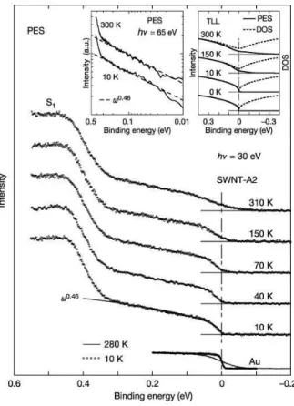
The LL paradigm applies to a variety of systems. Initially, quasi-one-dimensional condensed matter systems were suspected to belong to this cate- gory like the Bechgaard salts[78], and later carbon nanotubes, i.e. rolled up graphene sheets realized more faithfully LLs[79, 80, 81, 82, 83]. In particular, photoemission spectroscopy (PES) experiments[84, 85] probe directly the spectral functions in Eq. (1.28) and (1.30), yielding the non-integer power law exponents as shown in Fig. 1.16. Subsequent transport[86] as well as nuclear magnetic and conduction electron spin resonance studies[87, 88, 89]

have confirmed the adequacy of the LL picture. The edge states in integer and fractional quantum-Hall states form also one-dimensional object, and are described by the LL theory[71].

Recent years have witnessed a tremendous amount of experimental advances in cold atomic systems[63]. Trapping one-dimensional bosons or fermions offers the possibility to realize LL physics with the extra tunability of system parameters such as the inter-particle interaction (tunable by a Fes- hbach resonance or by changing the parameters of the optical trap) or the

(33)

Figure 1.16: The PES spectra of single-wall carbon nanotubes. The spectral function,|ω|^α (α = 0.46), broadened by the energy resolution, is indicated by a thick solid line in the spectrum at 10 K. The spectra of Au (3D conventional metal) are also shown. The left inset shows the PES, which were measured with an energy resolution of 15 meV athν = 65 eV, plotted on a loglog scale.

The right inset shows the photoemission spectra and the densities of states (DOS) calculated for the LL state in the metallic nanotubes.

various relaxation channels (i.e. no phonons or impurities wich are ubiquitous in condensed matter systems). Ultracold fermionic gases have been realized using several atoms such as⁴⁰K[90, 91, 92],⁶Li[93],¹⁷¹Yb-¹⁷³Yb[94],¹⁶³Dy[95]

and ⁸⁷Sr[96], and temperatures well in the quantum degeneracy regime were reached (T < 0.1 EF, with EF the Fermi energy). All these atomic systems feature tunable interactions. Among these, 1D configurations have been realized using⁴⁰K[90, 91], ⁶Li[93], and the momentum distribution has been measured in time of flight (ToF) experiments in 2D[96] and 3D[92, 94]

Fermi gases. Therefore, by applying ToF imaging or momentum resolved rf

(34)

spectroscopy[90], the observation of the momentum distribution of Eq. (7.13) is within reach for 1D fermions [90]. Furthermore, the specific momentum distribution of a LL has already been observed in the Tonks-Girardeau limit of 1D Bose systems[70], which exhibit fermionic properties in this strongly interacting regime.

The peculiarities of 1D systems were first demonstrated in the so-called quantum Newton’s cradle experiment[69], sketched schematically in Fig. 1.17.

Already the classical, idealized Newton’s cradle when several balls are si- multaneously in contact, can only approximately be explained by just the exchange of specific momentum values[97]. A 1D Bose gas made of ⁸⁷Rb atoms, initially prepared in a highly out of equilibrium momentum superposition state of right- and left-moving atoms, was evolved in time without any noticeably sign of equilibration even after thousands of collisions. In 1D, such system with point-like interparticle interactions realizes the Lieb-Liniger gas[98], which is Bethe-Ansatz integrable. This means in this case, that there are as many constants of motion as degrees of freedom (i.e. Bose particles), therefore the system’s motion in phase space is restricted by the constants of motion. As a result, ergodicity breaks down and the gas does not thermalize, as was observed in the momentum distribution after several cycles, which re- tained a typical two-peak structure, characteristic to the initial state. When the same experiment was repeated using two- or three dimensional gases, which are not integrable, thermalization sets in immediately even within the first period.

Coupled condensates are also useful to mimic LL behaviour. Using atom chips, a 1D Bose gas with a few thousand atoms can be trapped in the 1D quasicondensate regime at very low temperature[67], and the 1D gas can be split into two 1D quasicondensates. Such a 1D quasi-condensate can be thought of as a LL, since the excitation spectrum grows linearly with the momentum. By the application of radio frequency (rf) induced adiabatic potential, the height of the barrier between the two condensates can be adjusted by controlling the amplitude of the applied rf field. This allows one to achieve both Josephson coupled and fully decoupled quasicondensates.

The fluctuations of the relative phase of the two condensates are measured by the coherence factor

Ψ(t) = 1 L

Z

dxexp [i(θ1(x, t)−θ2(x, t)]

, (1.54)

whereθ1,2 are the phases of the two condensates obtained after the splitting, respectively, and L is the length of the analyzed signal. This is predicted to behave, using a LL description, as Ψ(t) ∼ exp(−(t/t0)^2/3) with t0 a decay time constant.

(35)

Figure 1.17: a. Visualization of a classical Newton’s cradle[97]. b. Sketches at various times of two out of equilibrium clouds of atoms in a 1D anharmonic trap. Initially, the atoms are prepared in a momentum superposition state of right and left moving atoms. The two parts of the wavefunction oscillate out of phase with each other with a period τ. Each atom collides with the opposite momentum group twice every full cycle, for instance, at t = τ /2.

Anharmonicity causes each group to gradually expand, until ultimately the atoms have fully dephased. Even after dephasing, each atom still collides with half the other atoms twice each cycle.

(36)

Figure 1.18: Double logarithmic plot of the coherence factor, Ψ as a function of time for decoupled 1D condensates. Each point is the average of 15 measurements, and error bars indicate the standard error. The slopes of the linear fits are in good agreement with a 2/3 exponent, coming from a LL description, from Ref. [67].